Methodology of magnetic resonance imaging

Printed in Great Britain

Methodology of magnetic resonance imaging

R.R.ERNST

Laboratorium fiir Physikalische Chemie, EidgenSssische Technische Hochschule, 8092 Zurich, Switzerland

ABSTRACT 184

1. INTRODUCTION 184

2. N M R IMAGING 187

3. PRECONDITIONING PERIOD 191

4. TECHNIQUES FOR RAPID IMAGING 193

S- CLASSIFICATION OF IMAGING TECHNIQUES 195

5.1 Point-measurement techniques 196 5.2 Line-measurement techniques 196 5.3 Plane-measurement techniques 197 5.4 Simultaneous techniques 197 6. POINT-MEASUREMENT TECHNIQUES 197 6.1 Sensitive-point technique 197

6.2 Field focusing NMR (FONAR) and topical NMR 199 6.3 Volume-selective pulse sequences 200

6.4 Surface coils 201

7. LINE-MEASUREMENT TECHNIQUES 201

7.1 Sensitive line or multiple sensitive-point method 201 7.2 Line-scan technique 202 8. PLANE-MEASUREMENT TECHNIQUES 204 8.1 Projection—reconstruction technique 204 8.1.1 Reconstruction procedures 205 8.2 Fourier imaging 208 8.3 Spin-warp imaging 212 8.4 Rotating-frame imaging 213

8.5 Planar and multiplanar imaging 214 8.6 Echo-planar imaging 215

9. C O N C L U S I O N S 216

10. A C K N O W L E D G E M E N T S 2L6 1 1 . REFERENCES 2 1 7

184 R. R. Ernst

ABSTRACT

A survey of magnetic resonance imaging techniques is presented. Emphasis is put on the basic types of measurement procedures rather than, discussing all variants proposed so far. The general experimental procedure consists of two phases, the preconditioning period and the image formation period. While the preconditioning period determines the image contrast, the image formation process is responsible for image resolution. Means to improve sensitivity and to minimize measurement time are discussed.

I. INTRODUCTION

Medical diagnosis by magnetic resonance (MR) is in the course of gaining rapid acceptance by medical doctors. The potential for revealing insights into the human body seems almost unlimited. Magnetic resonance provides not only structural information but allows also the investigation of physiological processes. It can be used for clinical testing as well as for basic research on metabolic functions. It is likely to become a serious competitor of X-ray techniques and may open completely new approaches for medical diagnosis and in depth understanding of the basic processes on a molecular level.

The casual observer may be overwhelmed by the multitude of magnetic resonance methods that have been proposed so far for medical applications. This parallels the even greater richness of nuclear magnetic resonance (NMR) methods developed in the course of the past forty years for conventional spectroscopic investigations in physics, chemistry and biology (Ernst et al. 1987). There is hardly another discipline capable of matching NMR in terms of the number of proposed useful approaches, schemes, and tricks. While for most other techniques a single optimized standard procedure has evolved that is routinely applied for a majority of investigations, MR continues to expand the palette of intriguing variants at a breathtaking rate. It is not astonishing that it is presently one of the fields with the largest number of submitted patent applications. The situation finds its explanation in the easy realization of time domain experiments with an arbitrarily large number of radio-frequency pulses of freely selected shape, frequency, and phase, exploiting time-dependent magnetic fields and magnetic-field gradients.

The field of medical magnetic resonance can be divided into magnetic resonance

imaging (MRI) and magnetic resonance spectroscopy (MRS). The goal of MRI is

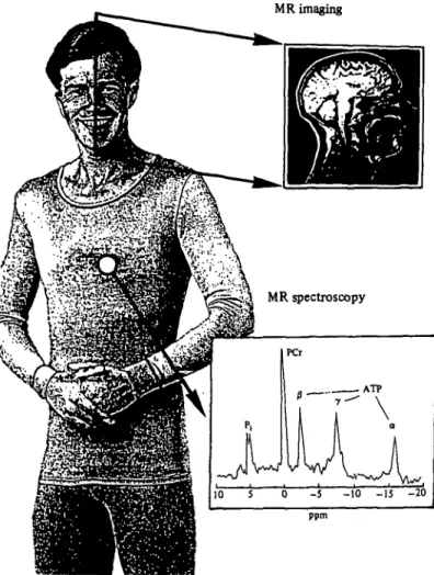
the production of images, by mapping cross-sections of the human body in analogy to X-ray computer tomography (CT) (see Fig. 1). Various parameters can be mapped, such as spin density, longitudinal and transverse relaxation times, the concentration of individual chemical components, as well as flow velocity of blood. MRS, on the other hand, provides spectral NMR information in a well defined volume element, and allows the detailed study of metabolic processes. The majority of spectroscopic investigations so far took advantage of 31P resonance.

However, promising studies are also feasible with 13C and proton magnetic

MR imaging MR spectroscopy 10

i

Jj

Fig. 1. Magnetic resonance imaging (MRI) and magnetic resonance spectroscopy (MRS). While MRI displays the spatial distribution of an NMR parameter, MRS presents a local spectrum. In this case, a phosphorus spectrum allows the distinction of inorganic phosphate (Pj), phosphocreatine (PCr) and adenosine triphosphate (ATP).

of the volume element to be addressed and depends in this respect on MRI techniques. In a second step spectral information is acquired in the frequency domain.

In this paper, we present an incomplete but representative survey of the available techniques. It is attempted to demonstrate the diversity of approaches by including also some examples which appear at present to be of rather historic interest. However, it is difficult to predict the tendencies and favours of possible future developments.

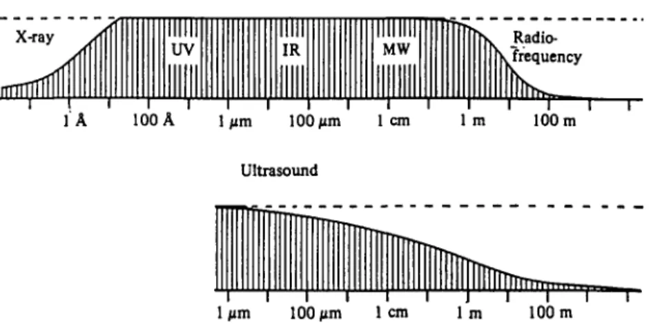
On first sight, it may not be fully obvious why macroscopic imaging should employ just the phenomenon of NMR and how such an imaging concept could be realized. Consider at first the attenuation of radiation by human tissue, schematically represented in Fig. 2 for electromagnetic and acoustical radiation. It is apparent that nature provides three windows which permit us to look ' non-invasively' inside the human body. The X-ray window has been exploited

186 R. R. Ernst Electromagnetic radiation X-ray UV IR MW l A 100 A 1/urn 100/un lcm l m 100 m Ultrasound l m 100 m

Fig. 2. Attenuation of radiation by human tissue. Electromagnetic radiation is strongly absorbed except in the X-ray and radio-frequency ranges. Acoustical radiation is absorbed except for the low-frequency range which is suitable for ultrasonic imaging. (Adapted from Ernst, 1986).

for more than 90 years starting with the basic experiments by Rontgen in 1895 and has completely revolutionized medical diagnosis. In recent years, CT had a further significant impact on medicine. Despite the potential dangers of the sizeable radiation dose, X-ray imaging is still one of the most important medical diagnostic tools.

The second window, which has been taken advantage of, is the low frequency ultrasonic window. It led to the development of ultrasonic scanners which produce images of acceptable quality in very fast sequence and allow the study of motional processes such as the cardiac cycle.

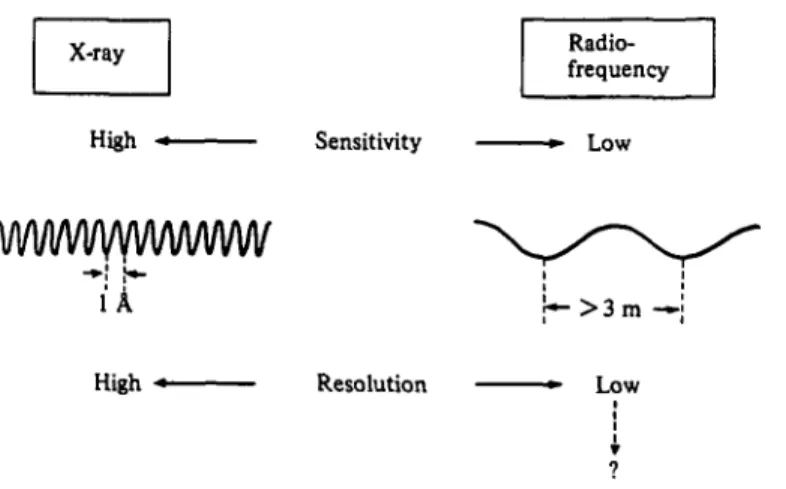
The radio-frequency (r.f.) window had not been exploited until 1972. This is not astonishing considering the achievable resolution, which in standard imaging procedures is limited by the wavelength of the applied radiation through the uncertainty relation. The maximum frequency useful for NMR imaging is in the order of 100 MHz, limiting resolution to about 3 m which is insufficient even for the imaging of full-grown elephants (Fig. 3). A fruitful application of NMR for imaging requires a completely new imaging concept.

The quantum energy involved in r.f. radiation is extremely low in comparison to typical chemical bonding energies, this is in contrast to X-rays which can easily rupture bonds and may induce destructive chemical processes (Fig. 4). MR is completely harmless.

The potential value of NMR for in vivo studies had been recognized already in 1971 by Damadian (Damadian, 1971, 1972). A feasible procedure for NMR imaging, was proposed in 1972 by Lauterbur (Lauterbur, 1972, 1973 a). He suggested the use of magnetic-field gradients to distinguish the signal contributions originating from various volume elements. In the years since 1972 numerous improved techniques of NMR imaging have been proposed. At present, the most

X-ray Radio-frequency

High Sensitivity Low

wwwvywwww

1A

High Resolution

Fig. 3. Radio-frequency irradiation in NMR uses much longer wavelengths than X-rays. This leads to low sensitivity and, in direct imaging procedures, to extremely low resolution. The sensitivity can be improved by optimized techniques, while the attainment of adequate resolution calls for a new imaging principle.

X-ray

Quantum energy

Radio-frequency

I

•

Fig. 4. The very low quantum energy of radio-frequency irradiation precludes adverse chemical effects in tissue, in contrast to energetic X-rays which can easily break chemical bonds and induce damaging chemical processes.

successful method is spin-warp imaging, that was introduced in 1980 by Edelstein

etal. (1980); and Johnson et al. (1983). It is a variant of Fourier imaging suggested

by Kumar et al. (1975 a, b).

2. NMR I M A G I N G

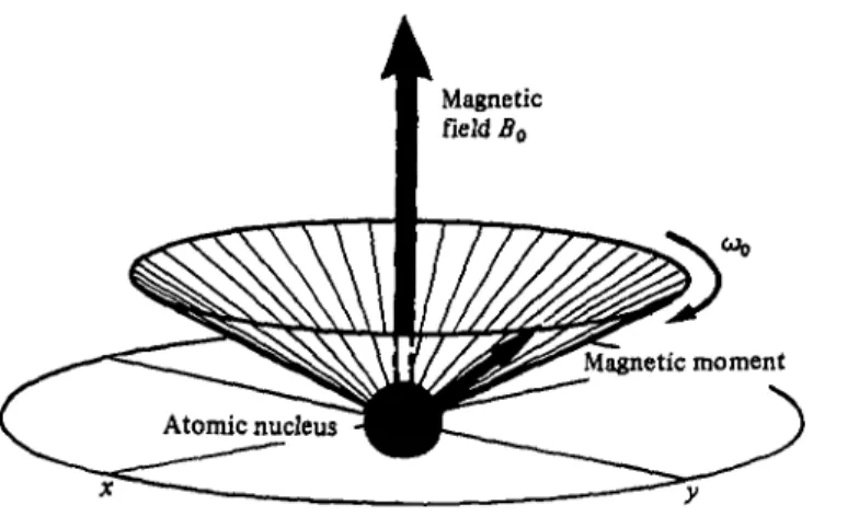
NMR imaging takes advantage of the magnetic moments of nuclei. The force acting on a nuclear moment ft placed in a magnetic field B represents the basic interaction which leads to NMR. In addition to the magnetic moment, the nuclei

188 R. R. Ernst

cot,

Fig. 5. The magnetic moment vector of an atomic nucleus precesses about the external static magnetic field Bo with the frequency w0 = — yB0.

M(t)

Fig. 6. The nuclear precession of Fig. 5 is damped by the two relaxation times Tx and T2.

Transverse relaxation leads to a decay of the precessing components Mx and My

proportional to exp{ —f/T4} with the transverse relaxation time Tt. Longitudinal relaxation

causes a recovery of the 2-component of the magnetization M proportional to i — exp{ — t/T,} with the longitudinal relaxation time Tv

90° Pulse

180° Pulse

n

Fig. 7. An on-resonance radio-frequency field Bl applied along the jc-axis causes a rotation

of the magnetization vector about the x-axis. An r.f. field pulse of length T = n/^yBJ leads to a 900 rotation ('900 pulse') while a pulse of length T = n/iyB^ causes a 1800 rotation ('1800 pulse').

possess a spin angular momentum. The resulting motion in a static magnetic field B is identical to that of a mechanical gyroscope and amounts to a precession with the angular velocity (Ernst et al. 1987; Abragam, 1961)

about the magnetic field direction (Fig. 5). The gyromagnetic ratio y is a measure for the size of the magnetic moment characteristic for a nuclear species.

The precession of a single magnetic moment u or of the entire magnetization M = i/vol Efc ftk in a volume element does not last indefinitely but is damped

exponentially with the transverse relaxation time T2. At the same time the

equilibrium magnetization Mo recovers exponentially with the longitudinal

re-laxation time Tj and aligns along the static magnetic field (z-axis) (Fig. 6). Normally T2 is much shorter than Tv

By the application of r.f. pulses it is possible to rotate the magnetization vector about any desired axis. For example, a r.f. field B1 applied for the time T along the X-axis rotates the magnetization vector by the angle /? = — yB^T about the

ioo R. R. Ernst

Fig. 8. Basic principe of NMR imaging. A magnetic field with increasing intensity along the x-axis is applied. The local resonance frequencies increases towards the right such that in a 'spectrum' the responses of the volume elements appear dispersed. Each spectral amplitude corresponds to the intensity originating from a cross-section through the object

perpendicular to the field-gradient axis. The spectrum displays a projection of the spin density onto the %-axis.

x-axis (Fig. 7). In many experiments %n and n pulses with /? = oo° and 1800,

respectively, are used. \n pulses are useful for rotating the equilibrium magneti-zation Mo from the position along the static field (z-axis) into the transverse (x,

y) plane for initiating free precession, n pulses, on the other hand, are needed for

the inversion of the magnetization in order to explore 7\ effects and can be used to refocus transverse magnetization.

NMR imaging relies on the usage of magnetic field gradients to disperse the NMR frequencies of the various volume elements of a medical object. The basic idea of NMR imaging is visualized in Fig. 8. A linear magnetic-field gradient applied along an axis of the object leads to resonance frequencies characteristic of the position along this axis. All volume elements in a plane perpendicular to the axis exhibit the same resonance frequency and contribute to the same signal amplitude. The NMR spectrum can thus be considered as a one-dimensional (1 -D) projection of the three-dimensional (3-D) nuclear spin density onto the direction of the field gradient. Normally proton magnetic resonance is used.

Additional experiments are necessary for the distinction of the volume elements within one of these planes. In effect a 3-D frequency space is required in which

Preconditioning Image formation

Contrast Resolution

Fig. 9. The two phases of an imaging experiment. Preconditioning is responsible for the image contrast, while the image formation process determines the spatial resolution.

each volume element of the object has its correspondence. Numerous experimental techniques have been proposed for establishing this correspondence.

A general imaging experiment consists of two phases which are often clearly separated in time (Fig. 9). The preconditioning or preparation period sets initial conditions for obtaining maximum image contrast in view of the question to be answered by the MR image. The second phase, the imaging period, serves to differentiate the various volume elements and determines the spatial resolution. Both periods affect the signal-to-noise ratio, although the selection of the imaging process is normally decisive in this respect.

3. PRECONDITIONING PERIOD

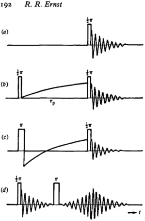
The image contrast can be influenced by several magnetic resonance parameters. The most important ones are the nuclear spin density p(r), the longitudinal relaxation time 7\(r) and the transverse relaxation time T2(r). In many cases all these parameters simultaneously contribute in a not always transparent manner to image contrast. It is however also possible to specifically design preconditioning processes in order to favour the influence of one of these parameters. Fig. 10 shows some commonly used preconditioning processes.

In the most simple case preconditioning consists just of a single preparation pulse, usually of rotation angle ft = \n (Fig. 10a) (Ernst et al. 1987). The magnetization is rotated into the (x, y)-plane and starts to precess under the influence of magnetic field gradients applied in order to differentiate the volume elements for imaging. When a sufficiently long waiting time T > 7^ is inserted between successive experiments to let the system fully relax, the image contrast will be determined primarily by the spin density p(r). However, for an insufficient waiting time, there is an additional influence of 7\(r).

In order to favour the influence of Tx(r) on image contrast, it is possible to simply

use a very fast repetition of the experiment of Fig. io(«). To ensure a well-defined initial state for longitudinal relaxation, one may apply an additional \ n prepulse, leading to the 'saturation recovery experiment' of Fig. 10(6). Here exclusively magnetization is imaged that has recovered during the time rp by Tj-processes.

Another Tj-sensitive experiment is the inversion recovery sequence of Fig. io(c) where a n prepulse initially inverts the magnetization. Its recovery proceeds through an intermediate zero value which can be exploited to suppress undesired

192 R. R. Ernst

(c) it

Fig. 10. Processes of preconditioning or preparation for manipulating the image contrast, (a) Single pulse creating transverse magnetization which leads to a free induction decay, (b) Saturation recovery experiment exploiting T, differences, (c) Inversion-recovery experiment also sensitive to Tx variations, (d) Spin-echo experiment for obtaining Ta-weighted images.

components with a characteristic 7\ value, by recording an image at this particular time.

Spin-echo experiments of the type shown in Fig. io(d) are sensitive to differences in the transverse relaxation time T2. The free precession is again started by a \n pulse. At £rp, a n pulse is applied which initiates refocusing of the effects

of magnetic-field inhomogeneities and of chemical-shift effects. An echo is formed at t = Tp at which time all magnetization vectors are again in-phase. ^-relaxation

however will lead to an irreversible decay of the magnetization which attenuates the echo amplitude. This can be exploited for T2-enhanced imaging.

The refocusing of magnetization by the application of n pulses is a general means for keeping the magnetization under control and is important in multi-echo imaging. By applying a repetitive sequence of n pulses after an initial %n pulse (Fig. u ) , it is possible to repetitively refocus the magnetization. Each echo can be recorded and used for a different image. Later echoes are increasingly weighted by differences in the transverse relaxation time T2. The various echoes, therefore, lead to images of different contrast. The entire set of images does not require more time than recording a single image as acquisition is performed within the idle waiting time.

II I I

nn n

II

i i

Fig. 11. Multi-echo multi-slice experiment. The experiment uses selective excitation of individual slices through the object. The signal obtained by a selective %n pulse from slice 1 is repetitively refocused by a series of n pulses. The echoes can be summed to enhance sensitivity or can be used individually for T2-weighted images. Before the magnetization in

slice 1 had time to fully recover, a second selective \n pulse is applied to slice 2. In practice many slices can be excited in the recovery time of the first slice.

Further improvement of the efficiency of data acquisition is possible by

multi-slice imaging as indicated in Figure. 11. The magnetization of slices not perturbed by the preceding slice selections can be excited without delay in the course of the waiting time. By this interlacing procedure it is feasible to record images of several slices without penalty in performance time.

Another type of refocusing of magnetization is exploited in the context of frequency-selective pulses applied in the presence of a magnetic field gradient for selecting a thin slice through the object. In the course of a long selective pulse, defocusing of magnetization components cannot be avoided. By applying a reversed magnetic-field gradient shortly after the pulse it is, however, possible to generate an echo and to recover the magnetization (see Section 5.2).

4. TECHNIQUES FOR RAPID IMAGING

So far it has been recommended to insert a waiting time at least of the order of

Tx for allowing the magnetization to recover between experiments. It has recently been recognized that high quality images can also be obtained with waiting times as short as T ~ TJ100. To compensate for the excessive saturation effect of such a rapid pulse sequence applied to the object, the pulse rotation angle ft has been drastically reduced, leading to what is sometimes called a FLASH technique (Haase

etal. 1986).

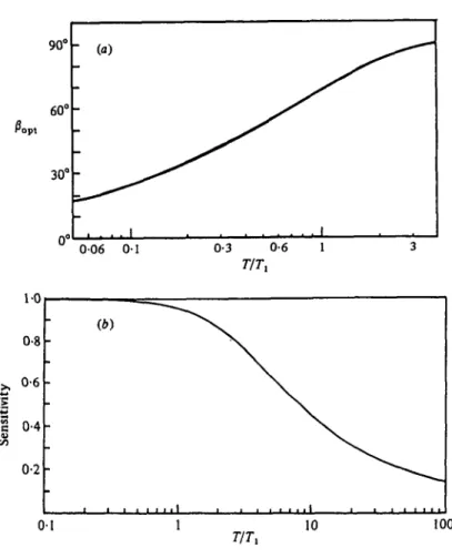
The rules governing the optimization of the pulse rotation angle ft for rapid pulsing have been explored in a different context earlier (Ernst & Anderson, 1966; Ernst, 1966): The results are as follows (Ernst et al. 1987):

194 R- R- Ernst

01

TIT, 10 100

Fig. 12. (a) Optimum pulse rotation angle /?opt for maximum signal intensity in a fast

repetitive pulse experiment with pulse delay T, shown as a function of T/Tv (6) Signal

intensity per unit time achievable in a fast repetitive pulse experiment with optimum pulse rotation angle /?opt.

(i) The optimum pulse rotation angle y?opt for obtaining a maximum signal in

a repetitive pulse experiment with pulse delay T is given by

(2) Given a total performance time Ttot, the maximum signal-to-noise ratio by

co-adding of signals is obtained for very rapid pulsing T <£ Tv However for

T < Tv no significant improvement can be attained by further shortening T as is evidenced by Fig. 12.

The selection of the pulse-rotation angle is not particularly critical specially when the selected angle surpases the optimum value stated above.

In another rapid imaging technique, called RARE (Hennig et al. 1984), excitation is achieved by a \n pulse and a number of independent experiments is performed in sequence by repeated refocusing by zr pulses. Each echo is recorded under a different phase-encoding gradient. In this way the performance time is reduced by the number of useful echoes. Adverse effects by the T2 decay of the echoes can often be tolerated or exploited for contrast enhancement. This type of technique

should be distinguished from the multi-echo method described above where each echo contributed to a different image. Here a single image is constructed using information gathered from all different echoes.

5. CLASSIFICATION OF IMAGING TECHNIQUES

The smallness of the nuclear magnetic moments and the low resonance frequencies lead to inherently low sensitivity of NMR. Indeed limited sensitivity represents the main obstacle for introducing more sophisticated imaging experiments and for observing nuclei different from protons. It is known that sensitivity can always be increased when more time is available for the measurement. In fact, the available signal-to-noise ratio S/N increases with the square root of the total performance time T (Ernst, 1966),

In clinical applications, the maximum permissible performance time T is clearly limited by patient-related considerations. To be of practical use, imaging experi-ments must be optimized in view of maximum sensitivity or minimum perform-ance time (Brunner & Ernst, 1979; Hoult & Lauterbur, 1979). Optimized

Point measurement

Line measurement

Fig. 13. Three types of imaging experiments, (i) Point measurement: each volume element is imaged separately. By sequential scanning a full image is obtained. No image

reconstruction is necessary, (ii) Line measurement: an entire line of N volume elements is simultaneously measured. From N independent measurements that contain information from all volume elements, the line image is reconstructed, (iii) Plane measurement: an entire plane of N2 volume elements is simultaneously measured. Each measurement is influenced by all JV* volume elements. An entire set of iV2 independent measurements allows one to unscramble the N2 contributions and to reconstruct an image.

196 R. R. Ernst

(a) (b) (c) (d)

Fig. 14. Four types of imaging experiments: (a) point-measurement techniques; (b) line-measurement techniques; (c) plane-measurement techniques, and (d) simultaneous techniques. (Reproduced from Brunner & Ernst, 1979.)

experiments always take advantage of the multiplex principle. By recording in parallel N channels of information, it is possible to reduce the performance time by a factor N. The multiplex advantage is the secret of success of many imaging techniques.

It seems appropriate to classify imaging techniques according to the number of parallel recorded channels. Three possible types of experiments are illustrated in Fig. 13. The simultaneously observed volume elements are sketched in Fig. 14.

5. i Point-measurement techniques

A single-volume element of the object is selectively excited and observed (Hin-shaw, 1974a, b, 1976; Damadian et al. 1977, 1978). For the construction of a complete image, one volume element after the other is scanned through sequen-tially. Point measurement techniques produce a direct image without any inter-mediate image processing. However, sensitivity will necessarily be low and the measurement time correspondingly long. Point measurement techniques are of particular merit when a localized area of the object must be investigated in great detail, for example for in vivo spectroscopy.

5.2 Line-measurement techniques

To increase sensitivity, an entire line of volume elements is excited and observed simultaneously as indicated in Fig. 13 (Hinshaw et al. 1977, 1978; Holland et al. 1977; Brooker & Hinshaw, 1978; Hinshaw, 1983; Andrew et al. 1977, 1978; Mansfield & Grannell, 1973, 1975; Mansfield et al. 1974, 1976; Mansfield & Maudsley, 1976 a, b, 1977 a; Garroway et al. 1974; Mansfield, 1976; Mansfield & Pykett, 1978; Hutchison et al. 1974, 1978; Sutherland & Hutchinson, 1978). A static magnetic field gradient is applied along this line to obtain the required frequency dispersion for distinguishing the volume elements that are simul-taneously observed. Line measurement techniques utilize normally a i-D pulse-Fourier experiment for simultaneous excitation. The computation of the line image merely requires a i-D Fourier transformation.

5.3 Plane measurement techniques

The sensitivity is further increased when an entire plane of volume elements is excited and observed at once as shown in Fig. 13 (Lauterbur, 1972, 1973 a, b, 1974a, b, 1977, 1979; Edelstein et al. 1980; Johnson et al. 1983; Kumar et al. 19750,6; Lauterbur et al. 1975; Mansfield &Maudsley, 1976c, 19776; Mansfield, 1977; Hoult, 1979). In some procedures, two-dimensional (2-D) image recon-struction can be achieved by a 2-D Fourier transformation (Kumar et al.

I

975fl> b). In other cases, more elaborate reconstruction procedures, for example filtered back-projection, are required (Brooks & Di Chiro, 1976; Shepp, 1980).

5.4 Simultaneous techniques

The most sensitive techniques involve simultaneous excitation and observation of the entire three-dimensional object (Kumar et al. 19756; Brunner & Ernst, 1979; Bernardo & Lauterbur, 1983). Such an experiment, however, can be quite demanding with regard to the amount of data to be acquired, and the necessary performance and data processing time can become excessive.

We shall describe in the following sections some prominent techniques for NMR imaging, classified according to the scheme discussed above.

6. POINT-MEASUREMENT TECHNIQUES

The selection of a single-volume element within an object can be achieved by three different approaches that may also be used in conjunction. These approaches are

(a) selective excitation of a volume element; (b) non-selective excitation and

selective destruction of unwanted magnetization; (c) selective observation of a single volume element.

Four such techniques will briefly be discussed. They are of particular merit for local spectroscopy rather than for imaging extended objects.

6.1 Sensitive-point technique

The sensitive-point technique proposed by Hinshaw (1974a, b, 1976) utilizes non-selective excitation pulses and defocuses all unwanted magnetization origin-ating from volume elements outside the selected one by means of time-dependent magnetic-field gradients.

The principle of the sensitive point technique is explained in Fig. 15. A continuous string of strong r.f. pulses of alternating phase is applied to the sample to create steady state transverse magnetization of all volume elements (Bradford

et al. 1951; Carr, 1958). At maximum half the equilibrium magnetization can

theoretically be maintained in a transverse steady state.

For the selection of the sensitive point at co-ordinates (x0, y0, z0), three time-dependent gradients are necessary. A sinusoidally modulated magnetic-field gradient gx(t) is applied along the x-axis such that its nodal plane passes through

(a)

Sensitive point (6)

90° -90° 90° -90° 90° -90° 90° -90° 90

Fig. 15. Sensitive-point technique: a sequence of r.f. pulses with alternating phases (6) generates a steady-state magnetization. Three time-dependent gradients (one of which is shown in (a)) modulate the resonance frequencies of all volume elements except for the sensitive point (intersection of the nodal planes of the alternating gradients). The modulation interferes with the formation of a steady-state magnetization, which is destroyed except for the sensitive point. (Adapted from Ernst et al. 1987.)

the point at x = x0 (Fig. 15). This gradient modulates the resonance frequencies of all volume elements lying outside the nodal plane. The modulation inhibits the formation of a steady state transverse magnetization and leads to destruction of the magnetization outside the plane x = x0. Two additional time-varying gradients

gy{t) and gz(t) are applied simultaneously along the other two axes with nodal planes

a t

y — 3>o anc* z = z0, respectively. When three incommensurate modulation frequencies are used, only the steady state transverse magnetization of the sensitive point remains and determines the observed signal.

By moving the three nodal planes, it is possible to move the sensitive point systematically through the object for obtaining a point by point image. The technique is quite slow. In particular, it should be noticed that after each measured point the magnetization must be allowed to recover before the next point can be measured. Consequently the data-acquisition rate is limited to about one point per

6.2 Field focusing NMR (FONAR) and topical NMR

For selecting a ' sensitive point' an alternative scheme has been used by Damadian

et al. (1977, 1978). In this technique, called FONAR, the static magnetic field is

shaped in such a way that good homogeneity is obtained only in a single small-volume element. The homogeneous region is normally near a saddle point of the field as shown in Fig. 16. Most of the object will give rise to a broad background signal, while the region around the saddle point gives a dominant contribution at one frequency. Additional contributions to the same frequency coming from the extended but narrow regions for ABQ = o may be negligible under suitable circumstances. The sensitive point is normally fixed within the magnet, and it is necessary to move the object to record a point by point image.

Field focusing NMR often does not lead to adequate spatial resolution for a high quality image, and it may be necessary to further enhance selectivity by suitably shaped radio frequency fields. The approach is useful, however, for in vivo spectroscopy in order to acquire spectral information (chemical shifts) of a localized area within an object. In the context of in vivo spectroscopy, this approach is known as 'topical NMR' (Gordon et al. 1982). It has been used intensely for recording resolved NMR spectra of a localized organ in a living being. It allows the study of physiological processes in a non-destructive and non-invasive manner.

Particularly 31P-NMR proved revealing for the measurement of metabolite

concentrations and pH in tissue (Gordon et al. 1980, 1982; Ackerman et al. 1980; Gadian, 1982).

Fig. 16. Shaping of the static magnetic field used in FONAR and topical NMR. Only the

region near the saddle point is sufficiently homogeneous to give rise to strong narrow signals, while the remainder of the object contributes only weak broad resonances.

200 R. R. Ernst

Although less resolution is required for in vivo spectroscopy than for imaging, such a simple field-focusing technique is often inadequate for investigating smaller organs, and alternative approaches have been proposed for better localizing the area of observation, as described below.

6.3 Volume-selective pulse sequences

The selective excitation of a single slice of an object can easily be achieved by applying a frequency-selective pulse in the presence of a magnetic-field gradient perpendicular to the desired slice. The selection of a single volume element however is more elaborate. It normally involves a three-step process whereby a point in the object is defined by the crossing of three orthogonal slices. This requires the intelligent combination of three 'slice-selective' pulses.

Aue et al. (1984, 1985) and Post et al. (1985) have recently described a clever technique for 'volume-selective excitation', illustrated in Fig. 17. By the simul-taneous application of a selective — \n and a non-selective \n pulse in the presence of a linear-field gradient, it is possible to rotate the entire magnetization outside of the selected slice into the (x, y)-plane where it decays by T2 processes. The

R.f.

r\

FID

Fig. 17. Sequence for volume-selective excitation (Aue et al. 1984, 1985; Post et al. 1985). Each of the three phases destroys the magnetization except within a single plane. In effect all magnetization, except for the selected plane, is rotated into the (x, y)-phne by the

combination of a selective and non-selective \n pulse. 7^-processes lead to the decay of transverse magnetization. At the end, magnetization in a single-volume element remains exclusively. It can be used for local spectroscopy by applying a further pulse in the absence of magnetic field gradients and observing the free induction decay.

magnetization in the selected slice remains unperturbed. After three pairs of such pulses in the presence of three orthogonal field gradients, only the magnetization in a single volume element remains. A final non-selective pulse in the absence of magnetic field gradients allows then volume-selective excitation and the observa-tion of a local NMR spectrum for a localized chemical analysis.

Volume-selective pulse sequences can be used for local spectroscopy anywhere within a medical object. However for an extended object, sensitivity will be relatively low because a large receiver coil must be used and the filling factor with regard to the selected volume element is small.

6.4 Surface coils

The sensitivity can be improved significantly by fitting the receiver and/or transmitter coils to the organ to be imaged or of which a spectrum must be recorded. In particular if observation of a volume element at or near the surface of the object is required, it is possible to employ ' surface coils' (Ackerman et al. 1980; Taylor et al. 1983; Bendall, 1986). A circular coil has a receptive volume approximately equal to a sphere with a diameter equal to that of the coil. Surface coils allow local spectroscopy without the need of applying magnetic-field gradi-ents. They lead to high sensitivity as the receptive volume fills the entire coil.

In a further refinement, it is possible to exploit the inhomogeneous r.f. field of a surface coil for enhanced spatial selectivity. An r.f. pulse of given duration and amplitude acts as a \n pulse only on a 2-D surface of constant r.f.-field strength. By properly shaping the pulses or using composite pulse sequences it is feasible to selectively excite approximately spherical calottes or differently shaped restric-ted areas of the object (Bendall & Gordon, 1983; Shaka & Freeman, 1984; Tycko & Pines, 1984).

7. LINE-MEASUREMENT TECHNIQUES

In line measurement techniques, a column of volume elements is selected. By means of a linear-field gradient applied along this line, the necessary frequency dispersion for distinguishing volume elements within the line can be obtained. A single-pulse Fourier experiment delivers simultaneously information on the entire line. In comparison to sensitive-point methods, substantial time saving can be achieved in this way, exploiting the multiplex advantage of Fourier spectroscopy (Ernst, 1966; Ernst & Anderson, 1966; Ernst et al. 1987).

7.1 Sensitive line or multiple sensitive-point method

The sensitive line or multiple sensitive-point (MSP) technique, suggested by Hinshaw (Hinshaw, 1983; Andrew et al. 1977), is a straightforward extension of the sensitive-point method. Instead of three time-varying gradients, only two time-varying gradients are used and a static-field gradient is applied along the 2-axis as shown in Fig. 18. Again steady-state free precession is generated by a

2O2 R. R. Ernst

B(x. t)

Fig. 18. The sensitive line technique applies time-dependent gradients along x and y directions, while a static gradient is applied along the 2-axis. The steady-state magnetization, generated by a sequence of pulses (see Fig. 156), is destroyed by the modulation except for volume elements in one column. (Adapted from Ernst et al. 1987.)

repetitive pulse sequence. The frequencies of precession between two successive pulses are analyzed in order to determine the spin density along the selected line. The sensitive-line technique is simple and leads to fair sensitivity. A few high-quality images using this technique have been obtained (Hinshaw et al. 1977; Andrew et al. 1978).

7.2 Line-scan technique

An inherent disadvantage of the sensitive-line technique is the complete saturation of all volume elements outside of the investigated sensitive line. Therefore, after each measured line, a waiting time has to be inserted before the next line can be excited. The disadvantage is shared with the sensitive-point technique.

The line-scan technique, proposed by Mansfield (Mansfield et al. 1976; Mansfield & Maudsley, 1976 a; Garroway et al. 1974) overcomes this deficiency (Fig. 19). At first, a single slice perpendicular to the *-axis is selected by applying a magnetic-field gradient along the x-axis and selectively saturating all volume elements outside this slice by means of tailored excitation (Tomlinson & Hill, 1973). A wide spectrum of frequencies is applied for saturation while the frequency of the selected slice is purposely suppressed to avoid saturation within this slice. A line perpendicular to the ;y-axis is then selected by a selective r.f. pulse in the presence of a y-gradient. Finally, the free induction decay of this line is observed in the presence of a z-gradient to disperse the responses of the volume elements

R.f. pulses

R.f. spectrum

Fig. 19. The line-scan technique (Mansfield et al. 1976; Mansfield & Maudsley, 1976a; Garroway et al. 1974) selects a plane by saturating all volume elements except for those in a plane perpendicular to the #-axis by tailored excitation (the r.f. spectrum should be white except for a 'dip'). A selective \n pulse in the presence of a y-gradient excites the

magnetization associated with a column of volume elements, and the signals originating from the entire column are recorded in the presence of a 2-gradient. (Adapted from Ernst et al. 1987.)

along this line. Because a selective pulse has been used for excitation, it is possible to immediately repeat the experiment on another line within the same slice without suffering from saturation effects.

It should be noted that after a selective pulse the various excited magnetization components show significant phase dispersion and may lead to mutual cancellation. The dispersion can be eliminated by the application of a reversed field gradient for a short time following the pulse (Sutherland & Hutchison, 1978; Hutchison

et al. 1978; Hoult, 1977; Mansfield et al. 1979). This allows the formation of an

echo where all magnetization components are again in-phase as shown in Fig. 20. A modified procedure, called echo-line imaging, that also leads to the selection of a single line has been indicated by Hutchison et al. (Hutchison et al. 1974, 1978; Sutherland & Hutchison, 1978).

2O4 R. R. Ernst

Fig. 20. In order to refocus the transverse magnetization components after application of a selective pulse, a reversed-field gradient is applied after the pulse. The resulting signal shows an echo where all magnetization components are again in-phase.

8. PLANE-MEASUREMENT TECHNIQUES

Medical imaging normally calls for planar sections through the object to be investigated. From the sensitivity standpoint, it is best to excite simultaneously an entire slice, leading to the planar techniques to be treated in this section. Extension to fully 3-D excitation techniques are straight forward. We will not devote a separate section to 3-D techniques, but include in this section a few remarks on extensions of 2-D techniques to three dimensions.

8.1 Projection-reconstruction technique

The projection-reconstruction technique has first been introduced into NMR by Lauterbur (Lauterbur, 1972, 1973a, b; 1974a, b, 1977, 1979; Lauterbur et al. 1975). In X-ray tomography this type of imaging is used routinely (Brooks & Di Chiro, 1976; Shepp, 1980). A spectrum of an object measured in the presence of a strong linear magnetic-field gradient represents a i-D projection of the object onto the direction of the applied gradient (Fig. 8). It is well known that three orthogonal projections are insufficient in order to construct a faithful image of the object. In fact, a large number of projections is required for computing a well-resolved image (Fig. 21). The number of projections recorded should match the number of resolution elements to be distinguished in one dimension in the case of 2-D imaging, or the number of resolution elements in two dimensions for 3-D imaging.

Let us restrict the discussion here to imaging in two dimensions. By means of a selective pulse applied in the presence of a magnetic-field gradient, e.g. along the «-axis, one entire plane perpendicular to the 2-axis is excited. The FID is then observed in the presence of a magnetic-field gradient applied along a line in the

Fig. 21. Projection-reconstruction technique. By applying gradients with a variable orientation to an object (in this case a phantom with two water-filled cylindrical volumes), a set of spectra is obtained that correspond to projections of the object from which the image of the object is reconstructed. (Adapted from Ernst, 1986.)

(x, y)-plane subtending an angle <j> with the x-axis. A whole set of FIDs for different

angles <j> covering the range from <j> = o° to <f> = 1800 is recorded. The signals are Fourier-transformed and yield the required projections. These are then subjected

to one of the reconstruction procedures described below. 8.1.1 Reconstruction procedures

Several techniques for reconstructing images from projections have been devel-oped for X-ray tomography (Brooks & Di Chiro, 1976; Shepp, 1980; Budinger & Gullberg, 1974). The same procedures can be used equally well for the recon-struction of NMR images.

A simple method of reconstruction is the back-projection technique. The intensity of each projection is back-projected into the image plane along the

206 R. R. Ernst

direction of projection. If the untreated projections are used for this purpose, a blurred image will be obtained. However, by suitable prefiltering of the projec-tions, it is possible to obtain a faithful image. This is the basic principle of filtered back-projection.

Another possibility is iterative reconstruction which also employs the procedure of back-projection (Budinger & Gullberg, 1974). However, after each cycle, new projections of the current image are computed and compared with the real projections of the object. The differences are again back-projected in order to improve the image iteratively. The recursive procedure leads to a faithful image without requiring prefiltering of the data.

The Fourier reconstruction technique reveals some basic features important in the following section in the context of Fourier imaging. It is based on the projection cross-section theorem: Let S(a)v w2) be the desired image of an object in two

dimensions and P(w, <j>) be a projection of the image obtained by applying a static gradient along a line at the angle <f>. The projection cross-section theorem then states that the i-D Fourier transform c(t, <j>) of the projection P((o, 0) represents

CO,

sit

Fig. 22. Projection cross-section theorem. The projection P(w, <p) of the image 5(wi, to2) = S(—ygxu —ygXi) onto an axis that subtends an angle <f> with respect to the wx axis is obtained by applying a gradient in the direction <j>. The i - D Fourier transform of P(u), (/>) is equal to a cross-section c(t, <f>) through the origin tl = /2 = o (central cross-section) of the 2-D Fourier transform s(tlt t2) of the desired image.

Cross-section \ O 0 ' o \ o < O 0 <\ ' 0 0 Jf 0 Ol0 / o 0 0/0 yr 0 0 T9 0 O o\ 0 O O Nl

Fig. 23. Fourier reconstruction technique. The spectra are observed in the presence of

gradients with different directions <f>, like in Fig. 21. They correspond to projections P(w, <j>) (top left), which can be Fourier-transformed to give cross-sections c(t, 0), with grid-points indicated by filled circles in the right-hand figure. These sampling points correspond to time-domain signals (free induction decays) obtained in the presence of gradients applied along the direction (j>. A regular grid (open circles) is obtained by interpolation, and a 2-D reverse Fourier transformation leads to the desired image (bottom left). (Adapted from Ernst et al. 1987.)

a central cross-section through the full 2-D Fourier transform s{tlt t2) of the image

Sio)^ o)2). The measured frequencies Wj and w2 are related to the spatial co-ordinates

xt and x2 through the relations

*< = - w1/ ( y g ) , 1 = 1, 2,

where g is the magnetic-field gradient applied to obtain the projections. The projection cross-section theorem is visualized in Fig. 22.

We can use the theorem to reconstruct an image from projections by the following three steps (Fig. 23):

(a) The measured projections P(w, <f>) for different directions <f> of projection are

individually Fourier-transformed leading to central cross-sections c(t, <j>) through the Fourier-transformed image s(tv t2).

(b) By means of an interpolation procedure, a regular grid of sample points of s(tv t2) is computed in the (tv t2) domain.

(c) A two-dimensional reverse Fourier transformation of s(tv t2) produces the desired image S(u)v 0)2).

208 R. R. Ernst

magnetic-field gradient permits a direct measurement of the central cross-sections

c(t, <f>), and step (a) in the above reconstruction sequence can be omitted. The only

step in this image reconstruction procedure that requires approximation is the interpolation procedure for obtaining a regular grid of sample points. It can be appreciated in Fig. 23 that the measured sampling points (filled circles) are more densely distributed around the central point, t1 = t2 = o, than in the outer parts of the (tv £2)-plane. This implies that the ' low-frequency components' or the

coarse features of the image are better represented than the finer details contained in the high-frequency components at larger tx and/or t2 values.

It is desirable to modify the measurement procedure to directly obtain an equally spaced grid of sampling points s(tlt r2). This is indeed possible by Fourier imaging

as described in the following section.

8.2 Fourier imaging

Fourier imaging (Kumar et al. 1975 a, b), remarkable by its conceptional simplicity, forms at present the most frequently used class of techniques for obtaining NMR images. The various volume elements are localized by three sequential measurements of the frequency co-ordinates <ov o)2 and w3 in gradient fields

successively applied along three orthogonal directions. By exploiting the multiplex concept it is possible to treat all volume elements at the same time and to achieve maximum sensitivity. The technique is losely related to 'two-dimensional spectroscopy' used in analytical NMR particularly for the analysis of the structure of biomolecules (Ernst et al. 1987).

Fig. 24. 3-D Fourier imaging: in the course of three consecutive phases, gradients are applied along the x, y and 2 directions, respectively. The local frequencies during the first two periods, which determine the x and y co-ordinates of the volume elements,

phase-modulate the signal which is observed in the third period in the presence of a z gradient. The x andy information is 'phase-encoded'. The parameters tx and tt are systematically incremented in a series of experiments. A 3-D Fourier transformation of the acquired data produces the image.

Fourier imaging allows full 3-D imaging but can also be reduced to a 2-D (planar) version. In the 3-D scheme, shown in Fig. 24, at first a non-selective pulse excites transverse magnetization in the entire object. In a first, so-called evolution period of length tv the magnetization precesses in the presence of a gradient gx. During the second evolution period t2, a gradient gy is applied. Finally, the precessing signal s(tx, f2, t3) is observed during the detection period as a function of t3 in the presence of a gradient gz. The precession frequencies during the three periods measure the displacement of the volume element along the three orthogonal directions. Having determined the three frequency co-ordinates together with the corresponding signal intensity allows a direct construction of the image. However a separate measurement of the three sets of frequencies under the three gradients would not serve the purpose as it would be impossible to identify the three frequencies belonging to the same volume element.

In Fourier imaging, the signal is observed exclusively during the evolution period t3. The two evolution periods (containing the information for the x- and

90°

Fig. 25. Schematic representation of 2-D Fourier imaging. The evolution period t, serves to phase-encode the x co-ordinate information while during the detection period t2 the

precession frequencies measure the y co-ordinates. The initial phases of the signal observed during the detection period maps, as a function of the parameter tlt the signal during the

evolution period (indicated by dots). The 2-D Fourier transformation of the data set s{tlt t2)

(c) •ACDCA*• •BDED8A* •QOEDAA* •AH D C - " ••DDD .. •BCCCOA* ACEtCHA* •OCDCB*" 0

kHz-Fig. 26. Fourier imaging of a phantom consisting of two water-filled capillaries with an inner diameter of 1 mm and a centre-to-centre separation of 22 mm, immersed in D2O. The

tubes are oriented parallel to the y-axis and aligned in the (x = o)-plane. (a) Time-domain signals: four typical free induction decays were recorded throughout evolution and detection periods (normally observation is restricted to the detection period). In the t, and t2 periods,

gradients were applied along the x- and z-axes respectively (in the tx period, the signals from

both tubes have the same frequency). (6) Signals S{tlt wa) obtained by i-D Fourier

transformation with respect to the t% time variable, (c) Signal 5(wlF w2) obtained after the

second Fourier transformation (absolute-value display). (Adapted from Kumar et al. 19756.)

^-directions) influence the observed signal through the initial phase. The information for the x- and ^-directions is 'phase-encoded' in the observed signal. By a systematic variation of the durations of the evolution periods ij and t2 it is possible to retrieve the 3-D signal s(tlt t2, t3) in which each volume element is represented by an additive contribution of the form

*(«i, h, h) = s(*> y>z) e xP ( - i

x, y, z being the co-ordinates of the volume element.

By means of a 3-D Fourier transformation it is possible to separate the contributions of the various volume elements

S(x, y, z) =

The principle of Fourier imaging is visualized in simplified form in Fig. 25 by restriction to two dimensions.

In practical 2-D Fourier-imaging excitation must be performed by a selective pulse applied in the presence of a gradient gx, called slice-selection gradient, to select a slice perpendicular to the jc-axis. In order to obtain a maximum signal, refocusing of the magnetization after the selective pulse is necessary by applying a reverse gx gradient simultaneously with the phase-encoding gradient gy during

i M

Fig. 27. Comparison of sensitivity to artifacts of projection reconstruction method and Fourier imaging. (PR) Projection reconstruction method applied to an object consisting of 33 circular disks. (FI) Fourier imaging applied to an object consisting of 32 square disks. (SW) Spin-warp imaging applied to an object consisting of 32 square disks, (h) Imaging in a homogeneous basic magnetic field, (i) Imaging in an inhomogeneous basic magnetic field with a maximum inhomogeneity of A50 = 0-4 g, where g is the gradient used for imaging in

T/cm. (ii) Imaging in an inhomogeneous basic magnetic field with a maximum inhomogeneity of AB0 = o-8 g. (Reproduced from Sekihara et al. 1984)

the evolution time. Observation is performed again in the presence of a read-out gradient gz.

Examples of recorded signals together with the results after each of two successive stages of Fourier transformation are shown in Fig. 26.

Fourier imaging and the Fourier projection-reconstruction technique are related. The two methods differ merely in the distribution of the sampling points in the 2-D or 3-D time domain. Fourier imaging yields an equally spaced grid of sampling points and leads therefore to equal accuracy in high- and low-image frequencies while the sampling points in the projection-reconstruction technique are concentrated near tx = f2 = o. Thus the finer details will be better represented

by Fourier imaging than in an image obtained with a projection-reconstruction technique.

That Fourier imaging is less susceptible to artifacts than the projection-reconstruction technique can be appreciated from Fig. 27. The images have been obtained in the presence of purposely introduced static field gradients that mimic

212 R.R. Ernst

an inhomogeneous magnet (Sekihara et al. 1984). While the projection-reconstruction technique leads to increasing blurring of the image for increasing field inhomogeneity, the Fourier imaging method merely causes a slight distortion of the otherwise clear image. The advantages in view of diagnostic applications are obvious.

8.3 Spin-warp imaging

Spin-warp imaging, proposed by Hutchison and co-workers (Edelstein et al. 1980; Johnson et al. 1983), represents a variant of Fourier imaging which turned out to be particularly easy to implement and has been very successful in commercial instruments.

Spin-warp imaging differs from conventional Fourier imaging by the fact that the phase-encoding period is fixed in length and that instead the amplitude of the applied magnetic-field gradient(s) is incremented from experiment to experiment. This has the advantage that relaxation effects during the phase-encoding time r remain the same through all experiments. The resolution in the phase-encoded direction is then independent of relaxation and exclusively limited by maximum available gradient field strength.

The experimental scheme of spin-warp imaging is shown in Fig. 28. The

R.f.

Fig. 28. Experimental scheme for spin warp imaging. In contrast to Fourier imaging (Figs. 24, 25), the phase encoding is obtained by increasing from experiment to experiment the amplitude of the gradient gy, rather than varying the duration of the evolution period r.

Fig. 29. Sagittal image of the author's head recorded by a procedure based on spin-warp imaging. (Courtesy of Radiologisches Zentrallaboratorium, Universitatsspital Zurich, Dr. G. K. Von Schulthess.)

excitation is effected by a selective r.f. pulse in the presence of a gx slice-selection gradient. During the phase-encoding period a reversed gradient —gx is applied to refocus the selectively excited magnetization. At the same time a phase-encoding gradient gy, which is incremented systematically from experiment to experiment, serves to obtain the differentiation of the volume elements in the y-direction. Finally during observation a read-out gradient, gz, is used to disperse the volume elements in the ar-direction. The gradients may be turned on and off in a smooth manner without adverse effects provided that the gradient shape is the same in all experiments of a series. A high-resolution image of a head recorded by spin-warp imaging is shown in Fig. 29.

Spin-warp imaging can easily be extended to three dimensions (Johnson et al. 1983). It can also be combined with chemical shift imaging.

8.4 Rotating-frame imaging

Another variant of Fourier imaging, proposed by Hoult (1979), combines prep-aration and evolution periods into one single interval. The transverse magnetiz-ation is excited by a linearly inhomogeneous r.f. field, e.g. with a gradient gx. Different planes in the object will experience different pulse rotation angles fi(x) (Fig. 30). A systematic variation of the pulse length (or amplitude) from experiment to experiment creates a characteristic amplitude modulation of the resulting signal

214 R.R. Ernst

Fig. 30. Rotating frame imaging: the evolution period consists of a pulse with an

inhomogeneous rf field with a gradient gx. The pulse width tx is incremented systematically,

leading to an amplitude modulation of the signal as a function of tx which depends on the

*-co-ordinate of the volume element. (Adapted from Ernst et al. 1987.)

which carries information on the #-co-ordinates. Detection takes place in the presence of a static read-out gradient gy.

Except for the replacement of a static-field gradient by an r.f. field gradient, rotating-frame imaging is fully equivalent to Fourier imaging. The same data processing is required. The major advantageof rotating-frame imagingis the absence of switched static-field gradients. This takes into account some concern about possible adverse effects of rapidly switched field gradients on human beings. On the other hand, it is more difficult to create a clean linear r.f.-field gradient. An extension to three dimensions without using switched static-field gradients is also not simple.

8.5 Planar and multiplanar imaging

A further imaging technique, called planar imaging, has been proposed by

described in Section 7.2. In contrast to line scanning, a set of parallel columns of volume elements are simultaneously excited by a suitably shaped multi-frequency pulse in the presence of a gradient gy. If sufficiently narrow strips of a selected plane are excited, it is possible to project the spin density on a single axis by the application of an inclined gradient such that the contributions of different columns do not overlap. Each column is then separately represented on the same axis.

Thus, a single experiment allows one to image an entire plane (although represented by narrow strips). Planar imaging is an exceptionally fast technique. The inherent trick is the reduction of the dimension by the mapping of an entire plane onto a single straight line. Although the idea behind this technique is quite ingenious, it has drawbacks. Sensitivity will be rather low, since very narrow strips of the plane have to be selected. In addition resolution is severly restricted because of the elongated shape of the distinct volume elements.

The technique can also be extended in the form of multiplanar imaging to three dimensions.

8.6 Echo-planar imaging

Echo-planar imaging, also proposed by Mansfield (1977) can be considered as another modification of Fourier imaging in which all experiments necessary to reconstruct the image of an entire plane are performed sequentially within a single FID. It is related to planar imaging but does not require selective excitation of narrow strips.

At first, transverse magnetization of an entire plane of volume elements is excited, e.g. by a selective pulse in the presence of a slice selection gradient gz. The

signal is observed in the presence of a weak static field gradient gx and a strong

R.f.

fl

Fig. 31. Echo-planar imaging: the magnetization of a planar section is selectively excited in the presence of a ^-gradient (not shown), and observed in the presence of a weak static *-gradient with a switched ^-gradient. (Adapted from Ernst et al. 1987.)

216 R.R. Ernst

switched gradient gy as shown in Fig. 31. This leads to a sequence of echoes due to the refocusing effect of the reversal of the field gradient.

To understand the principle and to grasp the relation to Fourier imaging, we can consider this procedure as a sequence of experiments, each experiment lasting from one echo peak to the next. The signal originating from a volume element at co-ordinates (x, y) in the wth experiment (following the nth echo) is then given by

s(nT, t

) = S(x, y) exp{-iyg

nT-iyg

t

},

where t2 = o at the top of the nth echo. The effects caused by gy in the previous periods have all been refocused, and the phase at time of the nth echo is entirely determined by the local field ygx. The signal s(nT, t2) is exactly the same as the signal s(tlt t2) in a 2-D Fourier-imaging experiment.

The reconstruction in echo-planar imaging also requires a 2-D Fourier trans-formation of the signal s(nT, t2). The method is one of the fastest and most sensitive techniques known today, as sufficient information about an entire plane is acquired during a single FID, reducing the time for a full image to about 100 ms. This allows, for example, studies of the cardiac cycle and renders possible real-time MR movies.

9. C O N C L U S I O N S

This survey of MR imaging techniques cannot claim completeness in several respects. Many variants of the basic techniques have not even been mentioned. In addition important fields such as flow imaging and microimaging are not covered. Fortunately, several excellent monographs .are available that provide more detailed and more extensive information (Mansfield & Morris, 1982; Jaklovsky, 1983; Kaufman et al. 1981; Wende & Thelen, 1983; Roth, 1984; Petersen et al. 1985; Morris, 1986; Partain et al. 1987).

It may have become obvious that the field of MR imaging is exceptionally rich in experimental techniques that fulfill various demands and provide an astonishing flexibility of the method. It is likely that almost any articulation of further needs will soon be matched by a corresponding methodological development. Indeed, the future of MR imaging looks at present truly unlimited in its potential to provide powerful tools for medical diagnosis.

10. ACKNOWLEDGMENTS

The author is indebted to G. Bodenhausen, A. Wokaun and Oxford University Press for the permission to adapt some of the material contained in chapter 10 of the monograph 'Principles of nuclear magnetic resonance in one and two dimensions' by R. R. Ernst, G. Bodenhausen and A. Wokaun; Clarendon Press, Oxford, 1987. The manuscript has been edited by Miss I. Miiller. The permission to reproduce Fig. 29, recorded by Dr G. K. Von Schulthess, University Hospital Zurich, is gratefully acknowledged.

I I . REFERENCES

ABRAGAM, A. (1961). Principles of Nuclear Magnetism. Oxford: Clarendon Press. ACKERMAN, J. J. H., GROVE, T. H., WONG, G. G., GADIAN, D. G. & RADDA, G. K.

(1980). Mapping of metabolites in whole animals by " P - N M R using surface coils. Nature 283, 167-170.

ANDREW, E. R., BOTTOMLEY, P. A., HINSHAW, W. S., HOLLAND, G. N., MOORE, W. S. & SIMAROJ, C. (1977). NMR images by the multiple sensitive point method: application to larger biological systems. Physics Med. Biol. 22, 971-974.

ANDREW, E. R., BOTTOMLEY, P. A., HINSHAW, W. S., HOLLAND, G. N., MOORE, W. S. & SIMAROJ, C. (1978). NMR imaging in medicine and biology. Proc. 20th Ampere

Cong. Tallinn.

AUE, W. P., MULLER, S., CROSS, T. A. & SEELIG, J. (1984). Volume selective excitation: a novel approach to topical NMR. J. magn. Reson. 56, 350-354.

AUE, W. P., MULLER, S. & SEELIG, J. (1985). Localized " C - N M R spectra with enhanced sensitivity obtained by volume-selective excitation. J. magn. Reson. 6 i , 392-396. BENDALL, M. R. (1986). Surface coil techniques for in vivo NMR. Bull. magn. Reson.

8, 17-42.

BENDALL, M. R. & GORDON, R. E. (1983). Depth and refocusing pulses designed for multipulse NMR with surface coils. J. magn. Reson. 53, 365-385.

BERNARDO, M. L. 8S LAUTERBUR, P. C. (1983). Rapid medium-resolution 3D NMR zeugmatographic imaging of the head. Eur. J. Radiol. 3, 257.

BRADFORD, R., CLAY, C. & STRICK, E. (1951). A steady-state transient technique in nuclear induction. Phys. Rev. 84, 157-158.

BROOKER, H. R. & HINSHAW, W. S. (1978). Thin-section NMR ranging. J. magn. Reson. 30, 129-131.

BROOKS, R. A. & Di CHIRO, G. (1976). Principles of computer assisted tomography (CAT) in radiographic and radioisotopic imaging. Physics Med. Biol. 21, 689-732. BRUNNER, P. & ERNST, R. R. (1979). Sensitivity and performance time in NMR imaging.

J. magn. Reson. 33, 83-106.

BUDINGER, T. F. & GULLBERG, G. T . (1974). Three-dimensional reconstruction of isotope distributions. Physics Med. Biol. 19, 387—389.

CARR, H. Y. (1958). Steady-state free precession in nuclear magnetic resonance. Phys. Rev. 112, 1693-1701.

DAMADIAN, R. (1971). Tumor detection by nuclear magnetic resonance. Science 171, 1151-1153.

DAMADIAN, R. U.S. Patent 3.789.832, filed 17 March, 1972.

DAMADIAN, R., GOLDSMITH, M. & MINKOFF, L. (1977). NMR in cancer: Fonar image of the live human body. Physiol. Chem. and Phys. 9, 97-100.

DAMADIAN, R., MINKOFF, L., GOLDSMITH, M. & KOUTCHER, J. A. (1978). Field focusing nuclear magnetic resonance (FONAR) and the formation of chemical scans in man. Naturwissenschaften 65, 250-251.

EDELSTEIN, W. A., HUTCHISON, J. M. S., JOHNSON, G. & REDPATH, T. W. (1980). Spin warp NMR imaging and applications to human whole-body imaging. Physics Med. Biol. 25,

751-750-ERNST, R. R. (1966). Sensitivity enhancement in magnetic resonance. Adv. in magn. Reson. 2, 1—135.

218 R.R. Ernst

ERNST, R. R. & ANDERSON, W. A. (1966). Application of Fourier transform spectroscopy to magnetic resonance. Rev. Set. Instrum. 37, 93-102.

ERNST, R. R., BODENHAUSEN, G. & WOKAUN, A. (1987). Principles of Nuclear Magnetic Resonance in One and Two Dimensions. Oxford: Clarendon Press.

GADIAN, D. G. (1982). Nuclear Magnetic Resonance and its Applications to Living Systems. Oxford: Clarendon Press.

GARROWAY, A. N., GRANNELL, P. K. & MANSFIELD, P. (1974). Image formation by a selective irradiative process. J. phys. Chem.: Solid St. Phys. 7, L457-462.

GORDON, R. E., HANLEY, P. E. & SHAW, D. (1982). Topical magnetic resonance. Prog. nucl. magn. Reson. Spectrosc. 15, 1—47.

GORDON, R. E., HANLEY, P. E., SHAW, D., GADIAN, D. G., RADDA, G. K., STYLES, P., BORE, P. J. & CHAN, L. (1980). Localization of metabolites in animals using 31P topical magnetic resonance. Nature 287, 736-738.

HAASE, A., FRAHM, J., MATTHAEI, D., HANICKE, W. & MERBOLDT, K.-D. (1986). FLASH imaging, rapid NMR imaging using low flip-angle pulses. J. magn. Reson. 67, 258-266. HENNIG, J., NAUERTH, A., FRIEDBURG, H. & RATZEL, D. (1984). Ein neues

schnellbild-verfahren fur die kernspintomographie. Radiology 24, 579.

HINSHAW, W. S. (1974a). Spin mapping: the application of moving gradients to NMR. Physics Lett. A48, 87-88.

HINSHAW, W. S. (19746). The application of time dependent field gradients to NMR spin mapping. Proc 18th Ampere Cong. Nottingham, p. 433.

HINSHAW, W. S. (1976). Image formation by nuclear magnetic resonance: the sensitive point method. J. appl. Phys. 47, 3709-3721.

HINSHAW, W. S. & LENT, A. H. (1983). An introduction to NMR imaging: from Bloch equation to the imaging equation. Proc. Inst. elect. Electron. Engrs. 71, 338-350. HINSHAW, W. S., ANDREW, E. R., BOTTOMLEY, P. A., HOLLAND, G. N., MOORE, W. S.

& WORTHINGTON, B. S. (1978). Display of cross-sectional anatomy by nuclear magnetic resonance imaging. Br. J. Radiol. 51, 273—280.

HINSHAW, W. S., BOTTOMLEY, P. A. & HOLLAND, G. N. (1977). Radiographic thin-section image of the human wrist by nuclear magnetic resonance. Nature 270, 722-723.

HOLLAND, G. N., BOTTOMLEY, P. A. & HINSHAW, W. S. (1977). 19F magnetic resonance imaging. / . magn. Reson. 28, 133-136.

HOULT, D. I. (1977). Zeugmatography: a criticism of the concept of a selective pulse in the presence of a field gradient. J. magn. Reson. 26, 165-167.

HOULT, D. I. (1979). Rotating frame zeugmatography. J. magn. Reson. 33, 183-197. HOULT, D. I. & LAUTERBUR, P. C. (1979). The sensitivity of the zeugmatographic

experiment involving human samples. J. magn. Reson. 34, 425-433.

HUTCHISON, J. M. S., GOLL, C. C. & MALLARD, J. R. (1974). In-vivo imaging of body structures using proton resonance. Proc. 18th Ampere Cong. Nottingham, p. 283. HUTCHISON, J. M. S., SUTHERLAND, R. J. & MALLARD, J. R. (1978). NMR imaging:

image recovery under magnetic fields with large non-uniformities. J. phys. Eng.: Sci. Instrum. u , 217-221.

JAKLOVSKY, J. (1983). NMR Imaging, A Comprehensive Bibliography. Reading, Mass.: Addison Wesley.

JOHNSON, G., HUTCHISON, J. M. S., REDPATH, T. W. & EASTWOOD, L. M. (1983). Improvements in performance time for simultaneous three-dimensional NMR imaging. J. magn. Reson. 54, 374-384.