HAL Id: hal-00508812
https://hal.archives-ouvertes.fr/hal-00508812
Submitted on 6 Aug 2010
HAL is a multi-disciplinary open access
archive for the deposit and dissemination of
sci-entific research documents, whether they are
pub-lished or not. The documents may come from
teaching and research institutions in France or
abroad, or from public or private research centers.
L’archive ouverte pluridisciplinaire HAL, est
destinée au dépôt et à la diffusion de documents
scientifiques de niveau recherche, publiés ou non,
émanant des établissements d’enseignement et de
recherche français ou étrangers, des laboratoires
publics ou privés.
Manifestation of ageing in the low temperature
conductance of disordered insulators
Thierry Grenet, Julien Delahaye
To cite this version:
Thierry Grenet, Julien Delahaye. Manifestation of ageing in the low temperature conductance of
dis-ordered insulators. European Physical Journal B: Condensed Matter and Complex Systems,
Springer-Verlag, 2010, 76 (2), pp.229. �10.1140/epjb/e2010-00171-9�. �hal-00508812�
Manifestation of ageing in the low temperature
conductance of disordered insulators
Thierry Grenet and Julien Delahaye
Institut Néel, CNRS & Université Joseph Fourier, BP 166, F-38042 Grenoble Cédex 9
published in the European Physical Journal B 76, 229 (2010)
PACS 72.80.Ng - Disordered solids
PACS 61.20.Lc - Time-dependent properties; relaxation PACS 73.23.-b - Electronic transport in mesoscopic systems PACS 73.23.Hk - Coulomb blockade; single electron tunnelling
Abstract – We are interested in the out of equilibrium phenomena observed in the electrical conductance of
disordered insulators at low temperature, which may be signatures of the electron coulomb glass state. The present work is devoted to the occurrence of ageing, a benchmark phenomenon for the glassy state. It is the fact that the dynamical properties of a glass depend on its age, i.e. on the time elapsed since it was quench-cooled. We first critically analyse previous studies on disordered insulators and question their interpretation in terms of ageing. We then present new measurements on insulating granular aluminium thin films which demonstrate that the dynamics is indeed age dependent. We also show that the results of different relaxation protocols are related by a superposition principle. The implications of our findings for the mechanism of the conductance slow relaxations are then discussed.
Introduction – Recently a set of out of equilibrium
phenomena was reported and studied in the low temperature conductance of disordered insulators like granular metals [1, 2], indium oxide [3] and ultra thin films of metals [4]. Macroscopic relaxation times were observed and an electronic origin was suggested for them, which opens fascinating questions as processes involving current carriers are generally thought to be fast. In practice, after the systems studied are cooled from room to liquid helium temperature, their conductance logarithmically decreases for days or weeks without any sign of saturation. If inserted in MOSFETs as their channel (see Fig 1 a), they exhibit an anomalous field effect which consists of a symmetrical minimum (thereafter called «the dip») in the conductance versus gate voltage (G(Vg)) curves (upper curve in Fig. 1 c).
The logarithmic decrease of G at fixed Vg observed after
cooling is associated with the progressive formation of a dip centred on that Vg value. The properties and slow dynamics
of the conductance dip have been studied in some detail in indium oxide [5, 6, 7, 8] and in granular aluminium [9].
An interpretation envisaged for these relaxation phenomena [5] rests on the concept of an electronic coulomb glass, a phase the carriers could constitute owing to their localized and interacting character [10]. One expects that the electronic coulomb glass possesses generic glassy dynamical features like ageing [11]. As a glass is out of equilibrium and endlessly evolves towards an equilibrium
state, its microscopic state is always changing and one expects that most of its properties evolve with time. In this paper we use the term ageing with the following meaning: ageing is the fact that during that never ending evolution the
dynamical properties of the glass evolve [12], it generally
responds more and more slowly to external stimuli. Several previous experiments have been interpreted as evidences of ageing in indium oxide [13, 14, 15, 6, 7] and by ourselves in granular aluminium [9].
In the present paper we first recall and critically discuss previous experiments and their interpretation. In particular we show that they cannot be taken as demonstrations of ageing according to the aforementioned definition of this term, as strictly speaking no unambiguous change of the
dynamics was revealed. We then present new relaxation
measurements on granular aluminium films using modified protocols, which demonstrate qualitatively new phenomena which we interpret as a clear signature of ageing. We explain why these could not be observed in previous experiments, and we show how the relaxations in different experimental protocols can be related to each other by the application of a superposition principle. We finally discuss the implications of our work for the “electronic coulomb glass” and other competing interpretations of the conductance dip and its slow relaxation in disordered insulators.
Critical analysis of previous “ageing” experiments – To
illustrate our discussion, we recall briefly the previous experiments on insulating granular Al thin films, similar to the ones also performed on indium oxide. We are interested in the slow response of the conductance to sudden gate voltage changes at low temperature. To look for ageing effects the following protocol was generally used (see Fig.1 b): Insulator Drain Source Granular Al Vg G Gate (a)
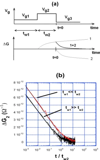
Fig. 1: (a) Scheme of a MOSFET like device used to measure the electric field effect in granular aluminium. (b) Scheme of the temperature and gate voltage sequences used in the “three step protocol”. (c) Illustration of the field effect anomalies and their dynamics. After the sample has been cooled to 4K with Vg = Vg1, a
dip forms during tw1, centred on Vg1 (upper curve). If Vg is then set to
Vg2 (2.5V in this illustration) a new dip forms while the first one
vanishes (second upper curve at tw1+tw2). If Vg is set back to Vg1 the
first dip is restored while the second one is progressively erased. We are mainly interested in the dynamics of the dip at Vg2. The
curves are shifted for clarity.
- First step: after the sample has been rapidly cooled from room temperature to T1=4K (with Vg1=0), a dip (we call dip
1) progressively forms in the G(Vg) curve and can be
visualized by performing a fast Vg scan like in the upper
curve of Fig. 1c. As the sample slowly proceeds towards equilibrium, the dip 1 amplitude increases like Ln(t) (t being the time since the fast cool).
- Second step: at time tw1, Vg is switched to Vg2 and the
formation of a second dip (dip 2) occurs while the dip 1 progressively vanishes (second upper curve of Fig. 1c).
- Third step: at time tw1+tw2, the gate voltage is set to a third
value Vg3, the dip 2 is consequently progressively erased
(two lower curves of Fig. 1c, where incidentally in this illustration Vg3 = Vg1).
We call this protocol the “three steps protocol”. It is similar to the isothermal-remanent magnetization (IRM) experiment used in the context of spin glasses (see for example [16]).
An important point is that these experiments were performed after the sample had long “equilibrated” with Vg=
Vg1, reaching a “quasi-equilibrium state” (i.e. tw1 >> tw2). It
was found that the writing of the dip 2 is history free (new dip amplitude increasing like Ln(t) ), while the dip 2 was erased as shown in Fig. 2. The erasure curves clearly depend on tw2 : the longer tw2 is, the longer it takes to erase
the dip 2. This was interpreted as ageing. Moreover it is seen that the erasure curves all precisely collapse on an “erasure master curve” when plotted versus t/tw2 (“full
scaling”), and the characteristic erasure time (defined as the intercept between the extrapolated logarithmic part and the abscissa axis, see inset of Fig.2) is equal to tw2. The same
observations were reported with indium oxide (see e.g. Figs 11 and 12(a) of [14]) 1. This dependence on tw2 of the
relaxation back to the quasi-equilibrium state was taken as a signature of “full ageing” (ageing with full scaling).
Fig. 2: Time dependence and full scaling of the vanishing amplitude of the dip 2 during the third step of the three step protocol (see text). Main graph: dip 2 amplitudes for tw2 = 1080 sec, 5400 sec,
27000 sec from left to right. The inset shows the perfect collapse of the curves plotted as a function of the reduced time t/tw2 (from [9]).
We now discuss these previous studies and point to their
1 To be precise in indium oxide the master function was measured by following the return of the dip 1 to its “equilibrated” amplitude after tw2. Since as long as tw1 >> tw2
(and in indium oxide as long as the Vg change is not too strong) the time evolutions of dips 1 and 2 are symmetrical [15, 9], the same master function as ours was
shortcomings. We first note that an actually more natural and simpler ageing protocol would be to restrict ourselves to the first and second steps of the three step protocol. Indeed if the dynamics of the systems does depend on their age, then the growth of the dip 2 during tw2 should depend on the
value of tw1. In particular if the system becomes “stiffer” due
to the growth of some internal correlations (the usual qualitative interpretation of ageing) one should observe that the writing of a new dip is slower when the system has spent a longer time in its glassy state. Thus the amplitude of the dip 2 written for a given tw2 should be smaller for longer
tw1. Unfortunately no such effect was reported yet nor was
observed by us previously, which questions the actual occurrence of ageing. One similar experiment was made with indium oxide in [7] (there called “T protocol”). Unfortunately the question of the tw1 dependence of the
growth of the dip 2 was not discussed. Instead a logarithmic extrapolation of the tw1 relaxation curves was subtracted
from the raw dip 2 growth curves. The resulting curves then of course strongly depend on tw1, but the justification of this
procedure is not clear to us and was not given in [7]. Actually we will show in the discussion section of the present paper how ageing (i.e. tw1 dependence of the
growth of the dip 2) may be discerned in the subtracted curves shown in [7].
Moreover the tw2 dependence and “full scaling” observed
with the three step protocol are not an undisputable evidence of ageing. One way to show this is to recall that one can reproduce the curves of Fig. 2 and their full scaling using a simple phenomenological model which does not incorporate ageing, as we have already shown and only briefly recall here. For more details see [9]. We supposed that a collection of reversible slow “degrees of freedom” influence the percolating conducting channels in the samples and that their relaxation “back” and “forth” can be induced by gate voltage changes. The precise nature of such degrees of freedom is not important for our argument. One may for instance think of localized polarisable tunnelling systems as has been considered in [9, 17]. Since the conductance relaxations observed are rather small (a few percents) we admit that the effects of the individual degrees of freedom are small and additive. Their relaxation times τi are exponentially dependent on the broadly
distributed parameters of the tunnelling barriers, which results in a 1/τi distribution of relaxation times. With these
simple ingredients one obtains the logarithmic growth of a new cusp and we showed in [9] that one also reproduces quite accurately the measured erasure curves and their full scaling without any fitting parameter. But this model does not incorporate ageing: the τi do not depend on the system’s
age. Actually the slopes of the logarithmic parts in Fig. 2 are all the same, which suggests that the dynamics of the erasure is the same in all cases and does not depend on
tw2. Obviously the difference between the curves simply
comes from the fact that they do not start from the same conductance value. The intercept of the logarithmic part of the erasure curves define typical erasure times that are equal to tw2. In other words it takes the same time to erase
the dip 2 as it took to write it, which sounds quite natural.
Thus as the experimental results discussed so far do not show any age dependence of the relaxation times at work, and can be reproduced using a simple model which does not incorporate ageing in that meaning, we conclude that they are not a demonstration of ageing.
Note for completeness that the 1/τi distribution is also
expected for the correlated coulomb glass model as was anticipated in [18] and was recently justified more quantitatively in [19], where the erasure phenomenology is also derived (to our point of view improperly referred to as “ageing”).
We now turn to our experimental program looking for ageing. It is simple in principle: systematically look for some effect of
tw1 on the dynamics of the dip 2 writing during tw2 (“two step
protocol”), and if any is found, look for the corresponding effect on the dynamics of the dip 2 erasure (“three step protocol”). We have of course no reason to restrict to tw1 >>
tw2 as was done in the previous experiments. We shall now
describe the results of such a study which we performed on granular aluminium films.
Experimental manifestations of ageing – The results
below were obtained studying two different samples which consist of field effect devices having a 200Å thick channel made of insulating granular aluminium. Sample A was prepared on a sapphire substrate on which an Al gate and a 1000Ǻ thick alumina gate insulator were deposited prior to the channel. Sample B was deposited on a doped silicon wafer, the 1000Ǻ thick thermally grown oxide layer acting as the gate insulator. The granular aluminium films had R
differences from the pure logarithmic relaxations, plotted versus t and t / tw1. The pure Ln(t) growth are determined for
each sample by the logarithmic part of the highest tw1 curve.
It is seen that the deviations from Ln(t) roughly scale with the time spent at Vg1. Another way to visualize the tw1
dependence is to look at the derivatives of the relaxation curves. This could only be performed after a Fourier transform filtering of the noise. It is seen in Figs. 3-c and 4-c that the derivatives exhibit a broad maximum which corresponds to the inflexion of the relaxation curves (in logarithmic scale) and which position also scales with tw1.
The departures from Ln(t) amount to roughly 10% of the observed relaxations. In spite of their limited amplitude, they constitute a qualitatively new phenomenon and show that the growth dynamics of dip 2 indeed depends on tw1, a clear
signature of ageing according to our definition of it.
This behaviour is reminiscent of e.g. ageing effects seen in zero field cooled magnetization relaxation experiments of spin glasses [20]. In this case the evolution of the relaxation curves was interpreted as the signature of an age dependent relaxation time distribution. The latter is usually computed as the derivative of the relaxation curves versus Ln(t), and exhibits a broad maximum centred on the samples age like in our case.
We used another procedure to demonstrate the age effect: measure, for different tw1 values, the dip 2 amplitude
obtained for a fixed duration tw2 spent with Vg = Vg2.
Practically the dip 2 amplitude was measured by switching the gate voltage to a value Vgref just after tw2 and measuring
the conductance jump induced (ΔG2), which is simply the
difference between the reference base line conductance (immediately measured at Vgref) and the bottom of the dip 2
(see Fig 5). The Vg2 and Vgref values were +5V and -5V
respectively for sample A, and +10V and -10V for sample B. The differential procedure ensures that the determination of ΔG2 is not significantly perturbed by possible slow drifts of
the He bath and sample temperature2.
Fig. 3:Ageing effect in the growth of the dip 2 in sample A. (a): dip 2 amplitude as a function of time for different tw1 values, from bottom
to top curves: tw1 = 6.85 104 s, 6000 s, 600 s and 10 s; (b):
departures from the pure Ln(t) growth as a function of t (left) and the reduced time t / tw1 (right); (c): derivative of ΔG2 as a function of
t (left) and the reduced time t / tw1 (right). The curves are shown for
two filterings to show that the broad maximum position does not depend on the amount of filtering.
2 We estimated that with this procedure the temperature drifts sometimes observed (a few mK during an experiment) could not influence the ΔG2 relaxations by more
Fig. 4:Ageing effect in the growth of the dip 2 in sample B. (a): dip 2 amplitude as a function of time for different tw1 values, from
bottom to top curves: tw1 = 3 104 s, 3000 s and 300 s; (b):
departures from the pure Ln(t) growth as a function of t (left) and the reduced time t / tw1 (right); (c): derivative of ΔG2 as a function of
t (left) and the reduced time t / tw1 (right).
This measurement was repeated for different tw1 (and the
same tw2). Between each measurement the sample was
heated up to 90K so as to erase any dip, the fast (not more than 10 seconds) cool down from 90K to 4K was realized by plunging it in the liquid He. The samples proved to be very stable upon this thermal cycling.
Fig. 5: Procedure used to investigate the effect of tw1 on the
amplitude of the dip 2 written for a given tw2. The sample is first
quenched to 4K and kept during tw1 with Vg = Vg1 (step 1). Then Vg
is switched to Vg2 and the dip 2 is formed during tw2 (step 2). Finally
Vg is set to Vgref and the amplitude of the dip 2 is determined as the
conductance jump ΔG2 induced by this last Vg change. In (a) we
schematize the G(Vg) curve which would be obtained if a fast Vg
scan was performed after the step 2 and indicate ΔG2 . In (b) we
show the actual conductance variations measured and indicate ΔG2.
In Fig. 6 we show the results of measurements performed with sample A. Here tw2 = 1350 s and tw1 was varied over
more than two orders of magnitude. One observes the ΔG2
dependence on tw1. As expected from Fig. 3 the longer the
sample was first aged at 4K with Vg = Vg1, the smaller the
achieved dip 2. The straight line in the figure is only a guide to the eyes, as one can expect that the effect saturates for large tw1 values3.
One may wonder what perturbation applied to the system after tw1 may rejuvenate it. Obviously, a change in gate
voltage Vg of a few volts does not have such an effect
otherwise the ageing would not be observable in our experiments (the age of the system would be erased when
Vg is switched from Vg1 to Vg2). This can be further
demonstrated in the following experiment: the system was aged for tw1a = 13500 s (i.e. 10tw2) at Vg1a = -2,5V and then
for tw1b = 2250 s (i.e. 1,67tw2) at Vg1b = +2,5V (for the
subsequent steps Vg2 = 7,5V and Vgref = -7,5V). It is seen in
3 Note that to describe the data, we mention tw1/tw2 values in order to specify the situations regarding the tw1<<tw2 and tw1>>tw2 limits. But we do not know whether the
Fig. 6 (filled triangle) that the ΔG2 value thus measured
corresponds well to the value expected for tw1≈10tw2 and
definitely not to tw1≈1,67tw2. Hence the gate voltage change
from Vg1a to Vg1b has not rejuvenated the sample, which age
is of the order of the total tw1a + tw1b. We do not know yet
whether much larger Vg steps can change the sample's age.
Fig 6: Effect of tw1 on the amplitude of the dip 2 formed during tw2 =
1350 s, for sample A. All steps performed at 4K unless specified. Filled circles show that the longer the sample was aged with Vg =
Vg1, the smaller the dip 2 amplitude. The filled triangle corresponds
to the sample aged at two different values of Vg1 (see the text), and
shows that the two ageing steps are cumulative (if not the experimental point would instead be the empty triangle). Filled squares correspond to the cases where an excursion to a higher temperature T* was imposed between 0.75tw1 and tw1. The higher
T*, the more the ageing at 4K between t=0 and 0.75tw1 is erased.
The T* values are: 6K, 8K, 12.5K, 16.5K, 20K, 26K, 36K and 46K. Error bars (shown on the left) are of the order of 2.10-13 Ω-1.
One may expect that the effective age of the system is modified by heating it. Such an effect is shown in Fig. 6. For this series of measurements a “high temperature” excursion was imposed during the ageing step (tw1). More precisely
the latter was performed in two steps, the first one for
tw1a=3960 sec (i.e. 2,9tw2) at the usual temperature T=4K
and the second one for tw1b≈1200 sec (i.e. 0,9tw2) at a higher
temperature which we call T*. The sample was then rapidly cooled back to T=4K and the gate voltage set to Vg2, the
rest of the procedure being as usual. A series of measurements was performed with T* ranging from 4K to 46K. The corresponding points are filled squares in Fig. 6: the higher T*, the larger ΔG2. We naturally define an
effective age of the sample as the ageing time which would have given the same ΔG2 if the whole process had been
performed at T=4K. In Fig. 7 one sees that the effective age of the system is approximately exponentially reduced by the high temperature T*.
We finally turn our attention to the “erasure master curve” which was under scrutiny in previously published three step experiments. We want to know whether it is also influenced by tw1. Recall we define the characteristic erasure time at
the intercept between the extrapolated logarithmic part of the ΔG2(t) and the time axis. As we already mentioned
above when tw1 is much larger than tw2, this erasure time is
found to be equal to tw2. However when tw1 is not very large,
we find that the erasure master function is modified: the full scaling is still obtained within our experimental accuracy but the erasure time is larger than tw2. This is shown in Fig. 8.
Thus for a “young” system it takes a longer time to erase a dip than it took to write it. This modification of the erasure master curve is the actual signature of ageing in the three step protocol.
Fig. 7: Effective ageing time (in units of tw2) as a function of T* for
sample A. The effective tw1 is defined as the ageing time which
would give the same ΔG2 would the ageing be performed at the
constant temperature T=4K. The effective tw1 is exponentially
reduced by the excursion at temperature T*.
Fig. 8: Erasure of the dip 2 as a function of t (time spent in step 3), when the gate voltage has been set back to Vg1 (sample B). The
master curves are obtained over more than 5 orders of magnitude of t/tw2 by superposing parts of it obtained with tw2 = 300 s, 3000 s
and 30000 s (the t/tw2 spans of the superposed parts are: 0.0024,
0.0240, 0.2200). Upper curve: the gate voltage was set to Vg2
upon quenching (i.e. tw1 = 0 s). Lower curve: tw1 was at least 15
times larger than the tw2 values. The erasure relaxation functions
are not the same for a “young” (upper curve) and an “old” (lower curve) sample. For a “young” sample, the curve starts from a more prominent dip 2 and the characteristic erasure time is larger than
One may expect that the relaxations studied in the two step and three step protocols are related. We now show that the “erasure master curves” of Fig. 8 can indeed be deduced from the growth curves of Figs. 3 and 4 using a superposition principle analogous to the one found in spin glasses [16]. For clarity ΔG2 will be denoted ΔGgrowth when
the dip 2 is being written and ΔGerasure when the dip 2 is
being erased. Let then denote the growth
with time t of a new dip which writing started after the sample spent a duration tw at low temperature. The
amplitude of a dip centred at some given Vg0 increases as
long as Vg is kept at Vg0, but it decreases if Vg is set at some
other value out of the Vg0 dip, as if a contribution of the
opposite sign was added. We may then expect the erasure curve of the three step protocol to obey the following relation (choosing the origin of the time scale t at the beginning of the third step):
(1) This procedure is illustrated in Fig. a. We show in Fig. 9-b two erasure curves computed from experimental growth curves of sample A (two step protocol) using Eq.1, in the two limiting cases tw1 >> tw2 and tw1 << tw2. Note that in the first
case ΔGgrowth doesn’t depend on tw1 and is logarithmic, so
that eq. (1) gives:
(2) This is just the erasure master curve predicted by the models mentioned in the previous section and shown to reproduce quite well the curves of Fig. 2 [9, 19]. However in the second case the ΔGgrowth are not exactly logarithmic and
the erasure curve computed from Eq. (1) is different. It is found to be similar to the measured erasure curve in Fig. 8. In particular the variation of the typical erasure time (extrapolation of the logarithmic part) with tw1 is well
reproduced. It is probable that using the superposition principle one can predict the relaxation following any gate voltage protocol once the experimental set of growth curves has been measured for a variety of tw
values.
Discussion – The experiments described above show that
the slow dynamics of the conductance dips depends on the system’s age. This is revealed by variations of the dip “growth” and “erasure” curves when “young” and “old” systems are compared. This could not be observed in previous experiments in granular Al [2, 9] and in indium oxide [13, 14, 15, 6, 7] which only focused on the erasure curve for very old samples (tw1>>tw2).
It would be interesting to know whether the ageing phenomena reported here also exist in indium oxide. One can find in [7] an indication that it may be so. Indeed if the
tw2 relaxation was exactly logarithmic in that case, the
subtraction of the logarithmically extrapolated tw1 relaxation
should result in ΔG ∝ Ln(1+tw1/t) (apart from the vertical shift
due to the normal field effect observed in InOx). The
logarithmic part of the resulting curve plotted versus t/tw1
should then extrapolate to 1 like in our lower curve in Fig. 8. However an inspection of the Fig. 2-b in [7] shows that, in spite of the scatter of the data, the scaled curves rather seem to extrapolate to t/tw1 larger than one. This means that
the tw2 relaxation in indium oxide also has a departure from
pure Ln(t) similar to ours. Note that according to our superposition principle the subtraction performed in the “T protocol” of [7] is actually a way to mimic the erasure curve in a three step protocol in the limit tw1<<tw2 and is thus
expected to extrapolate to a value larger than one. Note also that if we perform the same subtraction of Ln(t) to our
tw2 relaxation curves we of course get similar results.
Interestingly it was reported in indium oxide that when one applies Vg jumps [15] or non ohmic bias voltages [6] large
enough to erase previously formed dips, then modified erasure master curves are obtained. For moderately large perturbations, they are similar to the upper one in Fig. 8 and exhibit full scaling and an increased characteristic erasure time. This is fully consistent with our results and shows that such modified erasure curves are obtained either with “trully young” systems (this work) or with “old” ones which have been rejuvenated by applying a high enough electrical disturbance. The systems are effectively “young” when there is no well formed dip at any gate voltage.
What can we learn from these ageing effects about the microscopic origin of the dip and its slow relaxation? Two interpretations have been previously envisaged to explain it. In the first, as we recalled in the introduction of this paper, it is supposed that the charge carriers form a coulomb glass phase, and the field effect dip reflects the relaxation to equilibrium, a suggestion that has triggered numerous theoretical studies [19, 21, 11, 22]. These consider model systems where electrons are strongly localized and their coulomb repulsion is unscreened. The dip formation at constant Vg would then reflect the slow relaxation of the
glass towards its ground state for this Vg. In the case of
granular Al, the electrons are localized on the nanometric metal islands, and the slow relaxation of the electron glass would correspond to redistributions of electrons between the islands via correlated inter-island hopping.
In the context of granular metals, an “extrinsic” interpretation was also discussed [1, 23, 9]. The slow relaxation of conductance would possibly not be intrinsic to the charge carriers but be provoked by the slow relaxation of the disorder potential, which may be of atomic or ionic origin. It was shown that the slow relaxation of the dielectric polarization around the metallic islands (e.g. due to two level systems switching) could influence the coulomb blockade in such a way that the macroscopic conductance is reduced, thus creating a dip. A related model based on two level fluctuators was also suggested for the case of indium oxide [17]. However in the latter case, the effect of electron doping by oxygen deficiency is consistent with the electron coulomb glass scenario [24].
Fig 9: a – Scheme of the application of the superposition principle. Upper graph: Vg sequence of the three step protocol. Lower graph:
contributions to the amplitude of the dip situated at Vg=Vg2: “1” is
ΔGgrowth(t+tw2, tw1), “2” is -ΔGgrowth(t, tw1 + tw2) (see text). b - dip 2
amplitude as a function of the reduced time t/tw2 computed using the
superposition principle and the measured curves of Fig. 3 (tw2 =
6000 sec, tw1 = 10 sec and 6.85 104 sec). Note the similarity with
Fig. 8.
In [9] we noted that not only the extrinsic scenario, but also the coulomb glass one, can probably be described in terms of a collection of slow fluctuators influencing percolating conduction paths. This is suggested by the fact that the slow relaxation effects are observable in films close to the metallic state (with R
[19] AMIR A., OREG Y. and IMRY Y., Phys. Rev. B, 77 165207 (2008); AMIR A., OREG Y. and IMRY Y., Phys. Rev. Lett.,
103 126403 (2009)
[20] VINCENT E. in Ageing and the Glass Transition (Lecture
Notes in Physics) edited by HENKEL M., PLEIMLING M. and SANCTUARY R. (Springer, 2007)
[21] SOMOZA A. M. and A. M. ORTUNO A. M., Phys. Rev. B,
72 224202 (2005); SOMOZA A. M. et al., Phys. Rev. Lett.,
101 056601 (2008) ; YU C., Phys. Rev. Lett., 82 4074 (1999) ; TSIGANKOV D. N., et al., Phys. Rev. B, 68 184205 (2003) ; KOLTON A. B., GREMPEL D. R. and DOMINGUEZ D.,
Phys. Rev. B, 71 024206 (2005) ; MULLER M. and IOFFE L. B., Phys. Rev. Lett., 93 256403 (2004) ; LEBANON E. and MULLER M., Phys. Rev. B, 72 174202 (2005)
[22] KOZUB V. I. et al., Phys. Rev. B, 78 132201 (2008) [23] CAVICCHI R. E. and SILSBEE R. H., Phys. Rev. B, 38 640 (1988)
[24] VAKNIN A., OVADYAHU Z. and POLLAK M., Phys. Rev. Lett., 81 669 (1998)
[25] NESBITT J. R. and HEBARD A. F., Phys. Rev. B, 75 195441 (2007)