A hygrothermo-mechanical model for wood: part A. Poroelastic formulation and validation with neutron imaging : COST Action FP0904 2010-2014: Thermo-hydro-mechanical wood behavior and processing

*Corresponding author: Dominique Derome, Laboratory of Multiscale Studies in Building Physics, Empa, Uberlandstrasse 129, 8600 Dübendorf, Switzerland, e-mail: dominique.derome@empa.ch Saeed Abbasion: Department of Civil Engineering, ETHZ,

8093 Zürich, Switzerland

Jan Carmeliet: Chair of Building Physics, ETHZ, 8092 Zürich, Switzerland; and Laboratory of Multiscale Studies in Building Physics, Empa, 8600 Dübendorf, Switzerland

Marjan Sedighi Gilani: Applied Wood Materials, Empa, 8600 Dübendorf, Switzerland

Peter Vontobel: Spallation Neutron Source Division, Paul Scherrer Institute (PSI), 5232 Villigen, Switzerland

Saeed Abbasion, Jan Carmeliet, Marjan Sedighi Gilani, Peter Vontobel

and Dominique Derome*

A hygrothermo-mechanical model for wood:

part A. Poroelastic formulation and validation

with neutron imaging

COST Action FP0904 2010–2014: Thermo-hydro-mechanical wood behavior and processing

Abstract: The correct prediction of the behavior of

wood components undergoing environmental loading

or industrial process requires that the hygrothermal

and mechanical (HTM) behavior of wood is considered

in a coupled manner. A fully coupled poromechanical

approach is proposed and validated with neutron

imag-ing measurements of moist wood specimens exposed

to high temperature. This paper demonstrates that a

coupled HTM approach adequately captures the

varia-tions of temperature, moisture content, and dimensions

that result in a moist wood sample exposed to one-side

heating.

Keywords: energy method, finite element method (FEM),

heat and mass transport, hygrothermal and mechanical

(HTM) behavior, neutron imaging, poromechanics

DOI 10.1515/hf-2014-0189

Received June 30, 2014; accepted March 12, 2015; previously published online April 17, 2015

Introduction

An essential characteristic of wood as a porous material

of biological origin is its interaction with moisture. In the

hygroscopic domain, wood may sorb different moisture

contents (u) depending on the relative humidity (RH) of

the environment. The thermal gradients resulting from

exposing wood to heat lead to moisture transport. The

transport and storage of moisture and heat in wood are

interrelated to each other (i.e., dependent on both

temper-ature and u). Furthermore, changes in u result in swelling/

shrinkage and softening/hardening of wood.

Tempera-ture changes have similar dimensional and mechanical

effects, which are less pronounced.

One example for the hygrothermal and mechanical

(HTM) loading of wood is friction welding. Here, two

wood pieces are submitted to a relative motion to each

other parallel to the welded plane for a few seconds; the

joint interface heats up due to the friction, while, in a

small layer, plastic deformation and partial chemical

degradation occur. After cooling down, the two pieces

are fixed to each other. The glassy, natural bonding

interface formed of modified lignin and hemicelluloses

is strengthened by entangled wood fibers. In the present

paper, a mathematical modeling of the heat, moisture,

and mechanical aspects of the welding process is in

focus.

The literature describes the modeling of friction

welding for several materials, such metals, ceramics,

and polymers. Usually, modeling focuses on the thermal

effects and not on the mechanical effects. However,

Slu-zalec (1990) considered both effects, thus computing

strain and stress fields and temperature (T) distribution

in welded pieces. Fu and Duan (1998) applied the finite

element method (FEM) to analyze coupled deformation

and heat flow. D’Alvise et al. (2002) included contact

algo-rithm and automatic re-meshing at the joint interface and

considered a formulation for the friction law including

thermo-dependent material consistency. Lindemann et al.

(2006) modeled the bonding of aluminum with corundum

ceramic. For modeling wood-dowel rotation welding, an

analytical approach was applied (Zoulalian and Pizzi

2007), where the heat source term contains a constant

fric-tion coefficient. Ganne-Chédeville et al. (2008) developed

a numerical FEM to simulate the T behavior of wood pieces

during linear welding. The heat flow at the interface was

imposed to produce the T measured with infrared

ther-mography (IRT) at the side surfaces of two wood pieces

during welding. This model did not include mechanical

aspects.

The full welding process has been seldom analyzed

by FEM, but studies more and more consider both HTM

aspects of porous materials during welding. In the field of

cementitious materials, using the hybrid mixture theory,

Gawin et al. (2003) analyzed the hygrothermal behavior at

high T accounting for mechanical material deterioration.

Zeng et al. (2011) developed a poromechanical approach of

freezing behavior. The comprehensive model of Rémond

et al. (2007) links heat and mass transport to the

mechani-cal behavior of wood, but the model is not fully coupled.

The welding of wood is very complex, and the aim of

this paper is to propose a model that captures, in a first step,

the physical aspects involved in wood welding,

disregard-ing actual friction, and any chemical transformation. The

poromechanical approach will be applied to consider

simul-taneously the hygric, thermal, and mechanical (i.e., HTM)

behavior. The transport of heat and mass will be described

using T and capillary pressure gradients as the driving forces.

Then, a heating experiment will be documented based on

neutron imaging (NI), which was specially designed to allow

a validation of the proposed model. The subsequent paper

of this series is dealing with the application of the model in

parametric studies (Abbasion et al. 2015).

Computational model

The continuum approach of this study considers the macroscopic scale, where the porous wood appears to be homogeneous (i.e., where neither the different material components nor the cellular structure can be distinguished). However, in view of the growth ring structure of wood, a mesoscale feature is introduced to consider latewood (LW) and earlywood (EW). The orthotropic nature of wood is also taken into account. In this continuum approach, the porous material is considered to consist of three superimposed phases: (1) the solid phase (subscript s; i.e., the solid matrix), (2) the liquid phase (subscript l; i.e., water), and (3) the gaseous phase (subscript

g; i.e., moist air), which is a perfect mixture of two ideal gasses: dry

air (subscript a) and water vapor (subscript v).

Poromechanical approach

The poromechanics theory was introduced by Biot (1941) to take into account the interaction of fluids with the solid matrix. Coussy (1989,

1991, 1995, 2004, 2007, 2010) and Coussy et al. (1998) presented a general framework to formulate adequate constitutive equations for the poroelastic behavior. Here, a linear thermoporoelastic model is described first for unsaturated isotropic porous solids. The material is assumed to consist of a solid material (matrix) and a pore space partly filled by liquid water and a gas phase consisting of water vapor and dry air. The so-called Lagrangian porosity φ (Coussy 2007, 2010) relates the current porous volume of the material to the initial porous volume occupied before its deformation. The porosity is subdivided in the part filled by the liquid φl and the gas φg. The moisture con-tent (u) is defined as the ratio of liquid to dry material masses, or

u = ρ_lφ_l/ρ_o, with ρ_l and ρ_o representing the density of the liquid and the dry material, respectively. The pressures in the liquid and gas phases are pl and pg, respectively. The equivalent pressure, which is acting on the solid matrix, is denoted by p and can be obtained by incremen-tal volumetric averaging of the liquid and gaseous phases together, that is, φdp = φldpl+φgdpg or, in more common form, dp = dpg+Sldpc, where S_l = φ_l/φ is called liquid degree of saturation and p_c = p_g-p_l is the capillary pressure. The material is assumed to remain elastic and is initially stress free at an initial temperature T0 and pressure p0. Fol-lowing Coussy (2007), the free energy balance reads

ij

d d - d -d 0

ij p s T F

σ ε + φ = (1)

The first term refers to the elastic strain work related to the deformation of an infinitesimal element, with the σij (solid stress) and εij (solid strain) components. The second term accounts for the work supplied to the porous solid through its internal walls related to the change of porosity φ. The third term is related to energy change due to T change, with s being the entropy. F is the free energy of the solid matrix forming the solid part of the porous solid. Introducing the Legendre transform W of F

( , , ) ( , , )- _{ij ij}

-W σ p T F= ε φ T σ ε pφ (2) Equation (1) becomes

ijd ij dp s T Wd d 0

ε σ +φ + + = (3)

From Equation (3) the following is derived:

- ; - ; -ij ij W W _s W p T ε φ σ ∂ ∂ ∂ = = = ∂ ∂ ∂ (4)

Owing to the additive character of the energy W, it can be writ-ten as

2

1 1

-₂ ijkl ij kl-₂ - ( - ln )- ij ij - ij ij

-W= S σ σ Mπ C θ θ θ Bσ π α σ θ α πθφ (5)

The first term at the right-hand side of Equation (5) describes the elastic energy contribution, the second term the energy contribution of the fluid phases, and the third the energy change due to a change in T related to the heat capacity. The fourth term describes the energy contribution due to the fluid-solid interaction, and the fifth and sixth terms describe the elastic energy contribution due to a thermal dil-atation of the skeleton and the pore space, respectively. For linear poroelastic solids, the mechanical, thermal, and fluid terms read as in Equation (5), with π = p-p₀ and θ = T-T₀, where S_ijkl is the tensor of elastic compliances, M is the moisture capacity, C is the volumetric heat capacity, αij is the tensor of thermal dilatation coefficients, Bij is the tensor of moisture-mechanical coupling coefficients, and αϕ is the volumetric thermal dilatation related to the porosity.

Substituting Equation (5) in Equation (4), the state equations for linear poroelasticity are derived:

0 0 0 0 - ; -ij ij ijkl kl ij ij ij ij ij ij S B B M C s s _T φ φ ε ε σ π α θ φ φ σ π α θ α σ α π θ = + + − = + + = + + (6)

For isotropic materials, swelling and thermal expansion are assumed to be only volumetric, which means B_ij = 0, and α_ij = 0, when

i≠j. Equation (6) can then be written in terms of the mean stress σ,

mean volumetric strain ε, deviatoric stress s_ij, and deviatoric strain e_ij:

0 0 0 1

- S B 3 ; - B M φ ; e e_ij- _{ij 2}Ds_ij

ε ε= +σ π+ αθ φ φ = σ+ π α θ+ = (7)

where S is the bulk compliance, B is the moisture-mechanical cou-pling coefficient, M is the moisture capacity, and D is the shear compliance. Equation (7) can be rewritten in the more classical poroelastic form as presented by Coussy (2004):

0 0 0

- K -3 K b- ; - b p ; s s_{ij ij}- 2Ge_ij

N φ

σ σ = ε α θ π φ φ = + +ε α θ = ₍₈₎

where K is the bulk modulus, b is the Biot coefficient, N is the Biot modulus, and G is the shear modulus.

A nonlinear poroelastic model for unsaturated orthotropic porous solids is described starting with the constitutive equations. The solid is now assumed to be nonlinear elastic and orthotropic, as done in Carmeliet et al. (2013), and extending to include the T field. Using Equation (4) and with regard to symmetry of the second deriva-tive of W, the incremental state equations for strain, moisture con-tent, and entropy become

2 2 2 2 2 2 2 2 2 2 2 d - d - d - d d - d - d - d d - d - d - d ij kl ij kl ij ij ij ij ij ij W W _p W _T p T W W _p W _T p p T p W W W s _{T T p} p T T ε σ σ σ σ σ φ σ σ σ σ ∂ ∂ ∂ = ∂ ∂ ∂ ∂ ∂ ∂ ∂ ∂ ∂ = ∂ ∂ ∂ ∂ ∂ ∂ ∂ ∂ = ∂ ∂ ∂ ∂ ∂ (9)

Defining the thermoporoelastic properties

2 2 2 2 2 2 2 2 - - -- - -ijkl ij kl ij kl ij ij W W W S B _{p T} W W W M _{T p}C T p φ T α σ σ σ σ α ∂ ∂ ∂ = = = ∂ ∂ ∂ ∂ ∂ ∂ ∂ ∂ ∂ = = = ∂ ∂ ∂ ∂ (10)

the constitutive equations of the nonlinear porous solid are written as dε_ij=S_ijkldσ_kl+B p_ijd +α_ijdT (11a) dφ=Bijdσij+M pd +αφdT (11b) ds=α σ_ijd _ij+αφd Cd /p+ T T (11c)

For the nonlinear material, the thermo-poroelastic proper-ties Sijkl(σij, p, T), Bij(σij, p, T), αij(σij, p, T), M(σij,p,T), αϕ(σij,p,T), and

C(σ_ij,p,T) generally depend on stress, T, and effective pressure. Wood has two different pore systems: a fine nanosized one in the cell wall and a microscale pore network formed of the tracheid and ray lumens, which are connected by pits. In the cell wall at dry conditions, there is an initial porosity. Most of the porosity is, how-ever, created during the adsorption of water molecules and the swell-ing of the cell wall. In the followswell-ing, the cell wall is assumed to be always in saturated condition or Sl = 1.

The constitutive behavior as described by Equations (11a) and (11b) under well-defined experimental conditions is now analyzed. Consider a first experiment, where the material is brought in an environment with a certain gas (air) pressure pg, water vapor pres-sure p_v, and temperature T. The RH of the environment is defined as RH = pv/pvsat(T), where pvsat is the saturation vapor pressure related to

T. Assuming equilibrium between the external vapor pressure and

the vapor pressure in the pore space, Kelvin’s law describes the rela-tion between the pore vapor pressure (or RH) and the capillary pres-sure in the porous material:

(

)

exp c/ l v

RH= p ρR T (12)

where Rv is the ideal gas constant for vapor. As mentioned above, the cell wall is assumed to be saturated (Maloney and Paulapuro 1999, i.e., Sl = 1), and as experiments are performed at constant gas pres-sure (i.e., dpg = 0), the increments in effective pressure are equal to capillary pressure increments. Assuming a constant external vapor pressure and the material in immediate equilibrium, the effective pressure inside the material remains constant or dp = 0. A mechanical load is then applied and the strain and change of u are measured. Immediate equilibrium between the vapor pressure of the environ-ment and the pore space of the material is assumed. Equation (11a) then gives dεij = Sijkldσkl and Sijkl defines the elastic compliance, a meas-ure for the elastic strain capacity of the material. When the mechani-cal test is performed at different effective (or capillary) pressures and Ts, the compliance S_ijkl(σ_kl,p,T) dependent on stress, pressure, and T can be determined. The u increment is given by du = (ρl/ρ0)dφ. For constant pressure and T test conditions, Equation (11b) reads du = (ρl/ρ0)Bijdσij. The coupling coefficient Bij describes the change in

u due to an external mechanical stress. The influence of mechanical

stress on the sorption process is called the mechanosorptive effect. In a second experiment, the stress and pressure are considered constant (neglecting time-dependent behaviors such as creep) and the material is exposed to environments with different T. The strain and change of u are measured. Immediate equilibrium between the

T of the environment and the material is assumed. Equation (11a)

then reads dεij = αijdT and describes the thermal dilatation. Equation (11b) reads du = (ρ_l/ρ₀)αϕdT and describes the change in u due to T change, which defines the volumetric thermal dilatation related to the porosity.

In a third experiment, the stress and T are considered constant (once more neglecting time-dependent behaviors such as creep) and the material is exposed to environments with different external vapor pressure. The strain and change of u are measured. Immediate equi-librium between the vapor pressure of the environment and the pore space of the material is assumed. Equation (11a) then reads dεij = Bijdp and describes the change in strain due to a change in liquid pressure. The coupling coefficient B_ij thus describes the swelling/shrinkage of the material. Equation (11b) reads du = (ρl/ρ0)Mdp. M describes the change in u due to a change in effective (or capillary) pressure and is called the moisture capacity.

In a standard sorption test, the material is free of external load or σij = 0. The u measured in the unloaded condition is referred to as

u0, where the subscript 0 refers to the zero stress condition. The mois-ture capacity normally measured in unloaded condition is given by

(

)

for the nonlinear elastic material, the energy consists not only of quadratic terms but also of higher-order terms. According to Carme-liet et al. (2013), a general poroelastic description at constant T for orthotropic materials is given for wood. The compliance is found to be a quadratic function of the u or

0 1 2 0 ij ij ij S S B u= + (14) 1 ij

B terms refer to the first-order coupling between stress and u

in the energy equation of Carmeliet et al. (2013). The values for Sij are normalized to the compliance in the longitudinal (L) direction 0

11.

S

1

ij

B is normalized to the corresponding compliance 0

ij S to yield

(

)

with the dimensionless parameters a_ij and b_ij given by

0 1 0 0 11 , ij ij ij ij ij S B a b S S = = (16)

The swelling strain is assumed to be only volumetric, so

B₄₄ = B₅₅ = B₆₆ = 0. This assumption is correct for isotropic materials but is not proven for orthotropic materials. However, swelling in shear may be assumed negligible. The free swelling at stress-free conditions is given by 0

0

dε =_ii B u_iid , and the parameter B can be determined as 0ii the slope of the swelling strain versus u. Note that 0

ij

B describes the

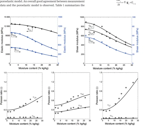
second-order coupling between stress and u (Carmeliet et al. 2013). Figure 1 compares measurements and curves obtained from the poroelastic model. An overall good agreement between measurement data and the poroelastic model is observed. Table 1 summarizes the

ETT ERR ELL GLT GLR GRT υLR υRL υRT υTR υLT υTL

Figure 1: Poromechanical model results (continuous lines) fitted with experimental modulus of elasticity (circles) reported by Neuhaus (1981). values determined for 0

11,

S a_ij, and b_ij. The coefficient a_ij spans a wide range from -0.29 to 222, showing the important orthotropic behavior of wood. The coefficient b_ij describes the moisture sensitivity of the compliance. The compliance is most moisture sensitive in the tan-gential (T) and radial (R) directions and much less in the L direction. The shear compliances are moisture sensitive, with a maximum in the RT direction. The off-diagonal compliances are very moisture sen-sitive. The swelling coefficient 0

ii

B is highest in the T direction, in the

R direction half this value, and in the L direction very low. The ortho-tropic moisture-dependent behavior of wood may be explained by its composition. The geometry of the individual cells and the arrange-ment/structure of the cells across the growth ring are responsible in large part for the anisotropy of swelling and stiffness, the archi-tecture of the cell wall layers and of the stiffer microfibril aggregates being the other factors affecting this anisotropy. Furthermore, at the mesoscale, the interaction of LW and EW may influence transverse anisotropy, as LW shows isotropic swelling, whereas EW swelling is greater in the T direction than in the R direction (Derome et al. 2011; Patera et al. 2013).

Heat and mass transport

For the conservation of mass in a porous material, the general mass balance equation for the mass component w_j (kg m-3_{) can be written as}

-j j i j w G t → ∂ = ∇⋅ + ∂ g (17)

-v g a a g g g g g g p ρ ρ ρ ρ   = + _ _   K D g ∇ ∇ (22b)

In terms of energy conservation, by neglecting the mechanical work and in the absence of any internal heat sources, assuming local thermal equilibrium, the energy balance reads

-j j j j j j h w h t ∂ = ⋅ + ⋅ ∂

∑

∑

where hj is the specific enthalpy of component j, q is the conductive heat flux vector that is described by Fourier law, with the T gradient as the driving force, and q = -λ∇T, in which λ is the thermal conductiv-ity tensor of the medium, as per Lewis and Schrefler (1998).

The material properties related to heat and mass transport are next defined. The dry densities of EW and LW are selected as 300 and 680 kg m-3_{. These values give an overall density of 376 kg m}-3 _{for dry} wood based on a volume fraction of 4:1 for EW and LW. The density of liquid water is dependent on both T and pressure. For water vapor and dry air, the ideal gas state equation, including both T and pres-sure dependence, is used. The density of the moist wood is based on the volume fraction of the mentioned densities, thus implicitly including both T and moisture effects.

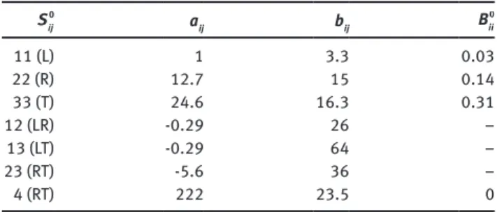
Moisture content u is a function of capillary pressure, or RH, and  of T. This hygroscopic curve is determined for the T range of 25–100°C from Weichert (1963) and by extrapolation to 250°C, as shown in Figure 2a.

The vapor diffusion coefficient is a function of RH, and as such also of capillary pressure and T, and given as an orthotropic tensor for EW and LW (see Figure 2b and c), according to Zillig (2009). The intrinsic liquid permeability is taken constant with a value at T = 296 K (Zillig 2009). The relative liquid permeability is given as a function of the saturation degree to the power eight for the L direction and power three for the transverse directions (Truscott 2004). The relative gas permeability decreases proportionally with the liquid saturation with power five in the L direction and power three in transverse direc-tions (Truscott 2004). The activation energy Ebw of the adsorbed water is a function of u in the hygroscopic range (Skaar 1998):

6 6 7 2 7 3

2.23 10 -3.95 10 1.62 10 -3.72 10 bw

E = × × u+ × u × u (24)

The effective thermal conductivity tensor is dependent on u and

T as reported by Kühlmann (1962) and is extrapolated to the range

of T considered here as follows. The thermal conductivity of wood is considered to be the superposition of the thermal conductivity of dry wood, water, and moist air. The thermal conductivity of dry wood increases linearly with T, whereas the thermal conductivity for both water and air is given as a function of T in thermodynamics tables. Therefore, the thermal conductivity of wet wood includes the effects of T and u. Note that the thermal conductivity of dry wood in the L direction is 2–2.5 times greater than in the transverse direc-tions. Similarly, the heat capacity of wet wood is given as a super-position of those of dry wood, water, and moist air (Forest Products Laboratory 2010).

The moisture-mechanical parameters are presented in Figure 1 and Table 1. The linear-logarithmic reduction of the stiffness with increasing T in the range of 0–200°C is accounted for by scal-ing the stiffness matrix with a function of T, f(T). Accordscal-ing to the Forest Products Laboratory (2010), the components of the ther-mal expansion tensor of wood can be described as αL = 4.1 × 10-6, α_R = 32.4 ×  10-9_ρ

dry+9.9 × 10-6, and αT = 32.4 × 10-9ρdry+18.4 × 10-6. Note that, where t is the time (s), gj is the flux vector (kg m-2 s-1), and Gi→j is

the rate of phase change from the phase i (source) to the phase j (sink; kg m-3 _s-1_).

For the liquid phase flow, a different transport mechanism is considered for each pore systems in wood (i.e., for cell wall and lumen). The cell wall is assumed to be in liquid-saturated state and the flux of (bound) water molecules is expressed by the diffusion equation. According to the activation energy of molecules in sorption sites, the effects of both the T and u are considered (Skaar 1998): - , ( - ) ( ) / bw bw bw bw bw bw v bw bw bw E u u T T u R T u E u T   =  _{∂ ∂} ∇ +∇      g D (18)

where subscript bw refers to the cell wall bound water, Dbw is the adsorbed liquid diffusivity tensor of the medium, and Ebw is the acti-vation energy of adsorbed molecules. In contrast to the bound water in the cell walls, the capillary transport in the lumens is described by Darcy’s law, indicating the pressure gradient as the driving force for convective transport:

(

)

(

)

( )

- , - ,

-fw= ρl l u T pfw ∇ =l ρl l u Tfw ∇ p pc

g K K (19)

where subscript fw refers to the free (bulk) water and Kl is the liquid permeability of the medium. Note that the gravitational effects are neglected in this equation.

For the gaseous phase flow, the gaseous phase (i.e., the mixture of water vapor and dry air) occupies only the lumen porosity and its transport mechanism includes bulk movement due to the pressure gradient as well as the diffusion of each component in the mixture. The convective (bulk) transport is described by Darcy’s law:

,conv. - ( , ) -( v a ( , )

g = ρgKg u T pg= ρg+ρg Kg u T pg

g ∇ ) ∇ (20)

where subscript conv. refers to the convective part of the flux, ρ_g is the density of gas phase, v

g

ρ is the density of water vapor, a g ρ is the density of dry air, and K_g is the gas permeability of the medium. The diffusive part of the flow is described by the Fick’s law of diffusion:

,diff. - ( , ) ( , ) - ,diff. v a g g v g g g g a g g u T ρ u T ρ ρ ρ ρ ρ     = _ _= _ _=     D D g ∇ ∇ g (21)

where subscript diff. refers to the diffusive part of the flux and Dg is the gas diffusivity tensor of the medium. Therefore, the flux vector of the water vapor and dry air can be written as follows:

- v - vg v g g g g g g p ρ ρ ρ ρ   = _ _   K D g ∇ ∇ (22a)

Table 1: Poromechanical parameters of wood, 0 11 S  = 1/(12 660 MPa). 0 ij S  aij  bij  Bii0 11 (L)  1  3.3  0.03 22 (R)  12.7  15  0.14 33 (T)  24.6  16.3  0.31 12 (LR)  -0.29  26  – 13 (LT)  -0.29  64  – 23 (RT)  -5.6  36  – 4 (RT)  222  23.5  0

due to a lack of data, all dependencies of the thermoporoelastic pro-perties on T, effective pressure (or u), and mechanical stress cannot be considered.

Finally, the system of coupled nonlinear equations is solved by means of the FEM method with an in-house code, which follows an iterative total incremental approach (Moonen 2009) and which is able to solve fully coupled hygrothermo-mechanical problems.

Validation experiment

Samples of spruce, a softwood with an average density

of 376 kg m

_{and dimensions 40  mm (height) × 80  mm}

(width) × 10 mm (thickness), are studied. The samples are

sawn side-by-side out of the same wood planks, oriented

so that the growth rings are visible during imaging and

that heat flow along the height occurs perfectly in the L, R,

or T direction. The samples are wrapped in Teflon tape to

prevent mass loss and covered with two foam glass plates

to minimize heat loss, at their vertical sides. The samples

are oven dried to determine their mass and then

condi-tioned until equilibrium in desiccators at 50% or 80% RH,

corresponding to equilibrium moisture content of 31 and

53 kg m

_{(i.e., 8% and 14% u).}

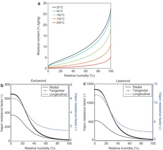
The setup for the heating experiment is shown in

Figure 3a. It consists of a frame that presses the sample

firmly against a metallic heating foil of 50 μm thickness

with two long bolts. The setup and sample are at 25°C at

the start of the experiment. Type E (NiCr-CuNi)

thermo-couples are placed below the foil on top of an

insulat-ing ceramic base and inserted in the samples. A power

supply of maximum power of 50 A and 120 V is applied

for foil heating and the base thermocouples serve to feed

back the T to the power supply controller. The control

system achieves a step increase to the desired foil T in a

few seconds followed by a perfectly maintained high T of

150°C or 250°C over the duration of the test. During the

test, the moisture and shrinkage behavior of the samples

are documented with neutron radiography and the Ts

detected with thermocouples are recorded by a data

acquisition system.

The NI facility of the Neutron Transmission

Radiog-raphy (NEUTRA) beamline at the Paul Scherrer Institute

(PSI), Villigen, Switzerland, was used for imaging and

0 5 10 15 20 25 30 0 20 40 60 80 100 Moisture content (% kg/kg) Relative humidity (%) 25°C 50°C 100°C 150°C 200°C 20 40 60 80 100 0 Relative humidity (%) 0 200 400 600 800

Vapor resistance factor (-) Vapor resistance factor (-)

0 2 4 6 8

Vapor resistance factor (-) Vapor resistance factor (-)

Earlywood Radial Tangential Longitudinal 20 40 60 80 100 0 Relative humidity (%) 0 500 1000 1500 0 5 10 15 Latewood Radial Tangential Longitudinal

b

a

c

Figure 2: Mass transport material properties: (a) sorption isotherms of spruce measured at 25, 50, and 100 from Weichert (1963) and extrapolated at 150°C and 200°C and vapor resistance factor of (b) EW and (c) LW for the orthogonal directions as a function of RH.

quantification of time resolved u in wood during the

heating experiment. This instrument relies on a neutron

beam within the thermal spectrum, with a most probable

energy level of approximately 25  meV (Lehmann et  al.

2001). The schematic overview is presented in Figure 3b.

The x- and y-axes correspond to the detector plane axes,

whereas the z-axis shows the neutron beam direction. The

detector consisted in a scintillator CCD camera system,

with a total field of view of 87 × 87 mm

_{. The scintillator}

is made of a 100-μm-thick sheet of zinc sulfide, doped

with

_{Li as the neutron absorbing agent, to convert the}

neutron signals into visible light photons. The photons

are then led via a mirror onto a cooled 16-bit CCD camera

(1024 × 1024 pixels). An initial neutron image is obtained

once the sample is set within the frame as the reference

image. Then, during the 20 min of the heating experiment,

neutron images are acquired at regular intervals of 16 s

with a spatial resolution of 100 μm.

The analysis of the neutron images for visualization of

the u distribution and their quantification is based on the

intensity measurements of the transmitted neutron beam

through an object. For a monochromatic beam, the

trans-mitted intensity I is described by the Lambert-Beer law:

- .

0 z

I I e

₌

(25)

where I

is the intensity of the incident neutron beam, z is

the total thickness of the object along the neutron beam

direction, and Σ is the effective attenuation coefficient.

Simplifying the composition of the samples consisting of

wood and water, a bilayer approximation is used where the

effect of moist wood on neutron attenuation is considered

equivalent to the effect of a water layer with thickness z

added to the dry wood sample (Sedighi Gilani et al. 2012).

Implementing this description, Equation (25) becomes

-{ . . }

0

( )

I t I e

₌

(26)

where subscript s refers to wood (solid) and w refers to the

equivalent water layer. At each time t during the

experi-ment, the change in the beam intensity with respect to the

initial stage results from a u change (i.e., the change in

“effective” water layer thickness in the bilinear model).

The u change from the initial state (water mass per volume)

is obtained by multiplying the change of effective water

layer thickness Δz

(t) by the water density ρ

and

divid-ing by the total sample thickness z

. Finally, the obtained

differential u in water mass per volume is divided by the

wood density to be presented in mass % (u).

A standard procedure, common to all radiation

trans-mission-based imaging methods, is used to correct raw

neutron images for artifacts. It includes correction for

back-ground noise of the CCD camera, for spatial fluctuations of

the incident beam, for scattering by the experimental

con-figuration and environment, and for polychromaticity of

beam energy spectrum. The Quantitative Neutron Imaging

algorithm developed at PSI (Hassanein 2006) is applied.

The desorption of water occurring during these

heating experiments results in the shrinkage of the wood

sample. u is obtained from the logarithmic subtraction of

the image taken at current time t from the initial image

taken at time t = 0. However, as the sample changes

geom-etry, the subtraction needs to be preceded by a registration

of the image. Registration is achieved with a bilinear image

registration algorithm, that is, TurboReg plug-in of ImageJ

(Thevenaz et al. 1998), to scale back the image and align its

edges with the edges of the reference image, at initial time.

Model validation

Boundary conditions and numerical domain

The calculation domain covers half of the specimens. In

addition, to reduce the simulation time, a 2D approach

is selected, assuming that the transport in the third

direction is negligible. The wood sample is divided into

several growth rings. For simplicity, all growth rings are

assumed to be of the same 3 mm width, where each ring

has an average density of 376 kg m

_{, with 2.4 mm of EW at}

300 kg m

_{and 0.6 mm of LW at 680 kg m}

_{(Figure 4).}

a

Vertical fixing screws

Heating plane CCD camera Mirror Detector Shielding Sample Collimator Neutron source

b

As seen in Figure 4, a constant temperature T

is

applied at the bottom. For the symmetry plane,

adiaba-tic boundary conditions for heat and no mass transfer are

considered. For the right boundary, which is in contact

with the environment, convective heat and mass transfer

occurs. Thus, the boundary conditions with this regard are

2.4 mm 3.0 mm

Convective heat and mass transfer Earlywood ρ=300 kg.m-3 _{ρ=680 kg.m}Latewood-3 T_base 40 mm 40 mm R L(or T)

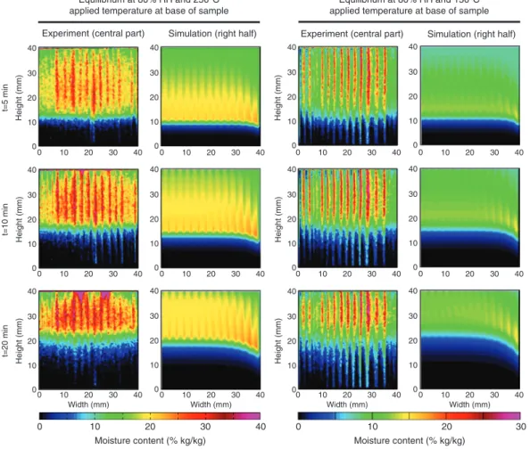
Figure 4: Computational domain and corresponding boundary conditions. 0 Moisture content (% kg/kg) 10 20 30 0 Moisture content (% kg/kg) 10 20 30 40 Equilibrium at 80% RH and 250°C

applied temperature at base of sample

Equilibrium at 80% RH and 150°C applied temperature at base of sample

0 10 20 30 40 Height (mm) 0 10 20 30 40 0 10 20 30 40 0 10 20 30 40 0 10 20 30 40 Height (mm) 0 10 20 30 40 0 10 20 30 40 0 10 20 30 40 0 10 20 30 40 Width (mm) Height (mm) Height (mm) Height (mm) Height (mm) 0 10 20 30 40 0 10 20 30 40 0 10 20 30 40 Width (mm) 0 10 20 30 40 Width (mm) 0 10 20 30 40 Width (mm) 0 10 20 30 40 0 10 20 30 40 0 10 20 30 40 0 10 20 30 40 0 10 20 30 40 0 10 20 30 40 0 10 20 30 40 0 10 20 30 40 0 10 20 30 40 0 10 20 30 40 t=5 mi n t=10 mi n t=20 mi n

Experiment (central part) Simulation (right half) Experiment (central part) Simulation (right half)

Figure 5: Moisture content distribution in the samples at different times, experimental results versus simulation results, in the R-L plane.

T , , , ,

( - )

( -

)(

( - )

)

( -

)( - )

h T T h p p

c T T

L

h c

p p

T T

⋅ =

+

+

+

n

q

(27a)

( -

)

⋅ =

n

h p p

q

(27b)

const.

p =

(27c)

where q

and q

are the heat and moisture flux vectors,

respectively; n is normal vector of the surface; T

is the

environment T; and h

and h

are the heat and moisture

convective transfer coefficients, respectively. The

mechan-ical boundary conditions include no displacement of the

symmetry plane in the R direction as well as fixing at the

top-left node; thus, the three surfaces are stress free.

Validation: u distribution versus time

The samples at equilibrium with 80% and 50% RH are

considered after 5, 10, and 20 min of exposure to base Ts

of 150°C and 250°C, in terms of u distribution in the RL

plane, comparing experimental and simulation results in

Figure 5. The heat front is clearly imaged with the sharp u

front that is propagating along the height of the samples,

at similar rate in both experimental and modeling results.

In the experimental results, the growth ring pattern is more

highlighted by the different u levels, and the u increase

ahead of the heat front is more important than in the

sim-ulation results. These differences can be attributed to the

higher inhomogeneity of the real material and some errors

in the image processing. The difference between the us of

EW and LW ahead of the heat front in the sample at 50%

RH is much less noticeable, indicating that the transport

properties considered, although adequate for the sample

at 80% RH, may have been different for this sample.

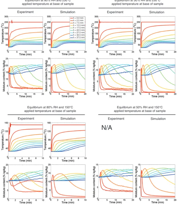
Validation: T and moisture content profiles

versus time

In this section, the average T and u across the samples are

compared; thus, the profiles of T and u versus time at nine

heights in the sample in Figure 6 are presented comparing

Equilibrium at 80% RH and 250°C applied temperature at base of sample

Equilibrium at 50% RH and 250°C applied temperature at base of sample

Experiment Simulation Experiment Simulation

N/A

applied temperature at base of sample

Equilibrium at 50% RH and 150°C applied temperature at base of sample

Experiment Simulation Experiment Simulation

h = 0.0 mm h = 2.5 mm h = 7.5 mm h = 12.5 mm h = 17.5 mm h = 22.5 mm h = 27.5 mm h = 32.5 mm h = 37.5 mm

Figure 6: Temperature and moisture content profiles versus time at nine heights in the samples, experimental results versus simulation results, in the R-L plane.

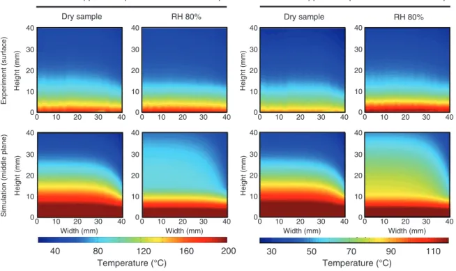
250°C applied temperature at base of sample 150°C applied temperature at base of sample 0 10 20 30 40 Height (mm) 0 10 20 30 40 0 10 20 30 40 0 10 20 30 40 0 10 20 30 40 Height (mm) Height (mm) Height (mm) 0 10 20 30 40 0 10 20 30 40 0 10 20 30 40 Width (mm) 0 10 20 30 40 Width (mm) 0 10 20 30 40 Width (mm) 0 10 20 30 40 Experiment (surface)

Simulation (middle plane)

Dry sample RH 80% Dry sample RH 80%

30 50 70 90 110 40 80 120 160 200 Temperature (°C) Temperature (°C) 0 10 20 30 40 0 10 20 30 40 0 10 20 30 40 0 10 20 30 40 0 10 20 30 40 Width (mm)

Figure 7: Temperature distribution in the samples at different times, experimental results versus simulation results, in the R-L plane.

experimental and simulation results for four different sets

of conditions. The T profiles come from the thermocouples

inserted in the sample. The u profiles are taken from the

calibrated neutron images presented in part in Figure 5.

u is averaged in narrow bands (0.50 mm thickness) across

the growth ring in the same height as the thermocouples.

Figure 6 shows very clearly that the global heat and

mois-ture behavior of the four samples as documented

experi-mentally is well captured by the simulations. In terms of

T, the rate of increase and the final values after 20 min

are correctly captured. The missing data of the sample at

equilibrium with 50% RH and exposed to a T of 150°C are

due to a computer malfunction during the experiment.

Regarding u, the increase of u ahead of the heat front is

very well captured as well as the length of the plateaus

and the rate of drying. However, the model does not

capture the residual u after drying.

Validation: surface T profiles versus time

To capture the T field of the sample during the heating

process, IRT is carried out by means of an NEC TH 3102

camera system with a Stirling cooler for dry sample and

moist sample (exposed to 80% RH), without insulation

to allow IR measurements. The T fields of four samples

from IRT and the corresponding plots from the modeling

are presented in Figure 7 at t = 10 min. Some differences

between the results from modeling and the

experimen-tal measurements are visible. In this experiment, in

con-trast to the NEUTRA experiment, the (larger) sides of the

samples are in contact with the environment, so there is

a considerable amount of convective heat loss from these

sides (i.e., heat transfer, which is not included in the

2D model). This effect is more considerable for the dry

samples because of lower heat capacity and thermal

con-ductivity of the medium. In addition, it should be noted

that the experiment results show the surface T, whereas

the model contours actually show the middle T

distribu-tion of the sample.

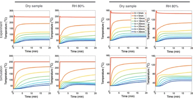
In this experiment, several thermocouples are also

embedded in the middle plane of the sample and at

dif-ferent heights. The recorded values by thermocouples and

averaged values at similar height from simulation are

pre-sented in Figure 8. From these figures, the role of water

on the formation of T plateaus is clearly illustrated, as no

plateau is seen in the T profiles of the dry samples.

Validation: shrinkage profiles versus time

Finally, to check the validity of the poromechanics

approach, the shrinkage profiles of the sample with 80%

RH and base T of 250°C are determined from the neutron

images and for different time steps evaluated by image

digitizing software. By considering these deformations of

the sample edge, it is possible to find the average strain

profiles of the sample along its height as (Sedighi Gilani

et al. 2014)

( , )- ( , )

( , )

( , )

L y t L y t

y t

L y t

ε

=

₍₂₈₎

where ε

(y, t) is the time-dependent average strain in the R

direction and L

(y, t) corresponds to the dimension of the

sample at time t along the R axis at a height position y. For

the model, the same equation is used to find the average

strain. The results are presented in Figure 9. As

demon-strated, both tensile and compressive strains occur along

the height of the sample, which is indicative of a bending

behavior. The moment causing this bending comes from

the induced internal stress due to the moisture loss, thus

related to pore pressure, at the region near the heat source

and the gain of moisture ahead of the heating front. In all

appearances, the negative strain zone is due to the hygric

effects and thus is considered to be shrinkage. However,

the positive strains could be due to the mechanical effects

of balancing the moment, not only at higher moisture

content, and thus may not be purely swelling strains.

Experiment

Simulatio

n

250°C applied temperature at base of sample 150°C applied temperature at base of sample

Dry sample RH 80% Dry sample RH 80%

Figure 8: Temperature profiles versus time at nine heights in the samples, experimental results versus simulation results, in the R-L plane.

Experiment Simulation

Figure 9: Average strain profiles in the R direction along the height of the sample at different time steps and for the sample with equilib-rium with 80% RH and Tbase = 250°C.

Conclusions

The exact prediction of the thermal, hygric, and

mechani-cal behavior of wood requires a holistic consideration

of several parameters. A fully coupled poromechanical

approach is proposed in the present paper and the

pre-dictions are validated with NI measurements of moist

wood specimens exposed to high temperature. It was

demonstrated that the model captures accurately the

vari-ations of moisture content, temperature, and dimensions

in the course of one-side heating. The model allows for

the implementation of different boundary conditions. The

implementation of the mesoscale features of the growth

rings (EW and LW) is necessary for exact predictions.

Acknowledgments: The contributions of Stefan Carl and

Roger Vonbank in developing the experimental setups are

acknowledged. Neutron radiography was performed at

Neutra beamline, SINQ, PSI, Villigen, Switzerland. SNF

Sinergia grant no. 127467 and the COST Action FP0904 of

the EU RTD Framework Programme are acknowledged.

References

Abbasion, S., Moonen, P., Carmeliet, J., Derome, D. (2015) A hygrothermo-mechanical model for wood: part B. Parametric studies and application to wood welding – COST Action FP0904 2010–2014: Thermo-Hydro-Mechanical wood behavior and processing. Holzforschung 69:839–849.

Biot, M.A. (1941) General theory of three-dimensional consolidation. J. Appl. Phys. 12:155–164.

Carmeliet, J., Derome, D., Dressler, M., Guyer, R. (2013) Nonlinear poro-elastic model for unsaturated porous solids. J. Appl. Mech. 80:020909.

Coussy, O. (1989) Thermodynamics of saturated porous solids in finite deformation. Eur. J. Mech. A Solids 8:1–14.

Coussy, O. Mécanique des Milieux Poreux. Technip, Paris, 1991. In English, Mechanics of Porous Continua. Wiley, Chichester, 1995. Coussy, O. Poromechanics. Wiley, Chichester, 2004.

Coussy, O. (2007) Revisiting the constitutive equations of unsatu-rated porous solids using a Lagrangian saturation concept. Int. J. Numer. Anal. Meth. Geomech. 31:1631–1713.

Coussy, O. Mechanics and Physics of Porous Solids. John Wiley & Sons, UK, 2010.

Coussy, O., Eymard, R., Lassabatère T. (1998) Constitutive model-ling of unsaturated drying deformable materials. J. Eng. Mech. ASCE 124:658–667.

D’Alvise, L., Massoni, E., Walloe, S.J. (2002) Finite element modeling of the inertia friction welding process between dissimilar materials. J. Mat. Proc. Technol. 125–126:387–391. Derome, D., Griffa, M., Koebel, M., Carmeliet, J. (2011) Hysteretic

swelling of wood at cellular scale probed by phase contrast X-ray tomography. J. Struct. Biol. 173:180–190.

Ganne-Chédeville, C., Duchanois, G., Pizzi, A., Leban, J.-M., Pichelin, F. (2008) Predicting the thermal behaviour of wood during linear welding using the finite element method. J.  Adhesion Sci. Technol. 22:1209–1221.

Gawin, D., Pesavento, F., Schrefler, B.A. (2003) Modelling of hygro-thermal behaviour of concrete at high temperature with thermo-chemical and mechanical material degradation. Comput. Methods Appl. Mech. Eng. 192:1731–1771.

Forest Products Laboratory (2010) Wood Handbook – Wood as an engineering material. General Technical Report. FPL-GTR-190. Madison, WI: U.S. Department of Agriculture, Forest Service, Forest Products Laboratory: 508 p.

Fu, L., Duan, L. (1998) The coupled deformation and heat flow analy-sis by finite element method during friction welding. Welding J. 77:202–207.

Hassanein, R. (2006) Correction methods for the quantitative evalu-ation of thermal neutron tomography. Ph.D. dissertevalu-ation, ETHZ Zurich, Switzerland.

Lehmann, E., Vontobel, P., Wiezel, P. (2001) Properties of the radiography facility NEUTRA at SINQ and its potential for used as European reference facility. Nondestr. Test. Eval. 16:191–202.

Lewis, R.W., Schrefler, B.A. The Finite Element Method in the Static and Dynamic Deformation and Consolidation of Porous Media. Second Edition. John Wiley & Sons Ltd., 1998, Reprint, 2000. Lindemann, Z., Skalski, K., Wlosinski, W., Zimmerman, J. (2006)

Thermo-mechanical phenomena in the process of friction welding of corundum ceramics and aluminium. B Polish Acad. Sci. 54:1–8.

Kühlmann, G. (1962) Investigation of the thermal properties of wood and particleboard in dependency on moisture content and temperature in the hygroscopic range (GER). Holz Roh- Werks. 20:259–70.

Maloney, T.C., Paulapuro, H. (1999) The formation of pores in the cell wall. J. Pulp Pap. Sci. 25:430–436.

Moonen, P. (2009) Continuous-discontinuous modelling of hygro-thermal damage processes in porous media. Ph.D. thesis, Katholieke Universiteit Leuven.

Neuhaus, F.H. (1981) Elastizitätszahlen von Fichtenholz in Abhän-gigkeit von der Holzfeuchtigkeit. Ph.D. thesis, Institut für konstruktiven Ingenieurbau Ruhr-Universität Bochum. Patera, A., Derome, D., Griffa, M., Carmeliet, J. (2013) Hysteresis

in swelling and in sorption of wood tissue. J. Struct. Biol. 182:226–234.

Rémond, R., Passard, J., Perré, P. (2007) The effect of temperature and moisture content on the mechanical behaviour of wood: a comprehensive model applied to drying and bending. Eur. J. Mech. A Solids 26:558–572.

Sedighi Gilani, M., Griffa, M., Mannes, D., Lehmann, E.,

Carmeliet, J., Derome, D. (2012) Visualization and quantifica-tion of liquid water transport in softwood by means of neutron radiography. Int. J. Heat Mass Transfer 55:6211–6221. Sedighi Gilani, M., Abbasion, S., Lehmann, E., Carmeliet, J.,

Derome, D. (2014) Neutron imaging of moisture displacement due to steep temperature gradients in hardwood. Int. J. Ther-mal Sci. 81:1–12.

Skaar, C. Wood-Water Relations. Springer-Verlag, Berlin, Germany, 1998.

Sluzalec, A. (1990) Thermal effects in friction welding. Int. J. Mech. Sci. 32:467–478.

Thevenaz, P., Ruttimann, U.E., Unser, M. (1998) A pyramid approach to subpixel registration based on intensity. IEEE Trans. Image Process. 7:27–41.

Truscott, S. (2004) A heterogeneous three-dimensional

computational model for wood drying. Ph.D. thesis, School of Mathematical Sciences, Queensland University of Technology. Weichert, L. (1963) Investigations on sorption and swelling

of spruce, beech and compressed-beech wood at temperatures between 20 and 100°C. Holz Roh- Werks. 21:290–300.

Zeng, Q., Fen-Chong, T., Dangla, P., Li, K. (2011) A study of freezing behavior of cementitious materials by poromechanical approach. Int. J. Solids Struct. 48:3267–3273.

Zillig, W. (2009) Moisture transport in wood using a multiscale approach. Ph.D. thesis (Eng.), Building Physics Laboratory, Katholieke Universiteit Leuven.

Zoulalian, A., Pizzi, A. (2007) Wood dowel rotation welding – a heat transfer model. J. Adhesion Sci. Technol. 21: 97–108.