Large hydropower and water-storage
potential in future glacier-free basins
Daniel Farinotti1,2*, Vanessa Round1,2, Matthias Huss1,2,3, Loris Compagno1,2 & Harry Zekollari1,2
Climate change is causing widespread glacier retreat1
, and much attention is devoted to negative impacts such as diminishing water resources2
, shifts in runoff seasonality3
, and increases in cryosphere-related hazards4
. Here we focus on a different aspect, and explore the water-storage and hydropower potential of areas that are expected to become ice-free during the course of this century. For roughly 185,000 sites that are glacierized at present, we predict the potentially emerging reservoir storage volume and hydropower potential. Using a climate-driven glacier-evolution model5
and topographical analysis6
, we estimate a theoretical maximal total storage and
hydropower potential of 875 ± 260 cubic kilometres and 1,355 ± 515 terawatt-hours per year, respectively (95% confidence intervals). A first-order suitability assessment that takes into account environmental, technical and economic factors identifies roughly 40 per cent of this potential (355 ± 105 cubic kilometres and 533 ± 200 terawatt-hours per year) as possibly being suitable for realization. Three quarters of the potential storage volume is expected to become ice-free by 2050, and the storage volume would be enough to retain about half of the annual runoff leaving the investigated sites. Although local impacts would need to be assessed on a case-by-case basis, the results indicate that deglacierizing basins could make important contributions to national energy supplies in several countries, particularly in High Mountain Asia.
Widespread glacier retreat is causing huge changes to glacierized landscapes around the globe1
. Further changes are already inevitable, with glaciers expected to lose a substantial fraction of their volume even if ongoing climatic warming were to stall7
. Under scenarios of high greenhouse-gas emission, glaciers are predicted to disappear almost completely in many regions8. Although negative impacts such as changing water availability2,3, cryosphere-related hazards4 and sea-level rise9 are well recognized, newly emerging ice-free basins have some-times been suggested to provide opportunities as well10–12. Increasing interseasonal water storage in newly deglacierized areas, for example, has been suggested as a possible mitigation measure against future seasonal water scarcity6
—an issue threatening the water security of millions of people who live downstream of mountain ranges hosting glaciers2,13,14. Similarly, projects to increase energy production and stor-age through hydropower installations in areas becoming ice-free have been proposed15, the flexibility and storage capacity of such schemes being recognized as valuable assets within the increasingly transient energy mix16
. Although the idea of constructing dams at former gla-cier locations might seem implausible at first, the lack of established human land use, the relatively simple ecosystem structures17
and the possibility of natural lake emergence11
may help to alleviate some of the environmental and social concerns typically associated with hydro-power development18,19.
Here we quantify the potential storage volume and hydropower pro-duction of glacierized areas that are projected to become ice-free within this century. By determining the technical potential and the suitability
of developing diversional hydropower plants at each individual glacier in the globally complete Randolph Glacier Inventory20
(RGI, version 6), we complement existing studies on the global hydropower potential of non-glacierized surfaces21
. We virtually place a dam wall at the low-est point of each glacier that is larger than 0.05 km2
and outside of the Sub-Antarctic (see Methods), and use digital elevation models of the subglacial terrain22 to simulate the reservoir storage volume of each of the roughly 185,000 sites selected in this way (see Extended Data Fig. 1 for a visualization). The lake volume per dam-wall area is optimized by varying dam orientation, length and height, the latter two parameters being constrained to remain within the range of already-existing, high-alpine hydropower infrastructure. The selection criteria are meant to minimize the impact on the landscape (rather than maximizing eco-nomic revenue, for example) while maximizing the reservoir volume and thus the flexibility in reservoir operations for both hydropower production and water management. The extent and timing of areas becoming ice-free are provided by the Global Glacier Evolution Model (GloGEM)5
, which is driven by 14 global climate models based on three representative concentration pathways (RCPs)23
. Annual potential hydropower production during the period 2017–2100 is estimated using projected basin-runoff from GloGEM and the available hydraulic head—the latter being determined as the maximum elevation drop from the virtual dam location to the surrounding topography (see Methods). Drawing on principles outlined by the Hydropower Sustainability Assessment Protocol24, we also provide an initial assessment of the suitability of every site. We consider a series of independently rated 1Laboratory of Hydraulics, Hydrology and Glaciology (VAW), ETH Zurich, Zurich, Switzerland. 2Swiss Federal Institute for Forest, Snow and Landscape Research (WSL), Birmensdorf, Switzerland. 3Department of Geosciences, University of Fribourg, Fribourg, Switzerland. *e-mail: [email protected]
http://doc.rero.ch
Published in "Nature 575(7782): 341–344, 2019"
which should be cited to refer to this work.
Turbine Dam Operation Piping Technical equipment Power station Miscellaneous Powerline 1.0 0.8 0.6 0.4 0.2 0 0.0 0.1 0.2 0.3 0.4 0.5
Production cost (USD kWh–1)
Cumulative hydr
opower potential (PWh yr
–1
)
d
Maximum cumulative hydr
opower potential (PWh yr
–1)
Maximum potential storage (10
3 km 3 ) 0.8 0.6 0.4 0.2 2.0 1.5 1.0 2020 2050 2080 Year RCP 8.5 RCP 4.5 RCP 2.6 c 1 10 102 103 104 0.8 0.6 0.4 0.2 0
Cumul. number of sites
PWh yr –1 b 1.4 1.2 1.0 0.8 0.6 0.4 0.2 0 0 25 50 75 100 125 150 175 Cumulative number of sites (thousands)
Cumulative hydr opower potential (PWh yr –1) ≥ 80 ≥ 70 ≥ 60 ≥ 50 ≥ 0 Suitability score Panel b a
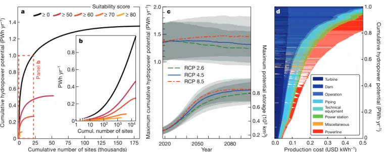
Fig. 1 | Global hydropower and water-storage potential from deglacierizing areas. a, Cumulative hydropower potential for a given number of sites (1 PWh = 103
TWh). Differently coloured lines depict different suitability-score thresholds. b, Enlargement of the indicated frame (note the logarithmic x-axis). c, Temporal evolution of the maximal cumulative hydropower potential (top) and reservoir storage volume (bottom). Results are shown for three
representative concentration pathways (RCPs) and include 95% confidence intervals (grey shading). Note that the displayed global averages mask regional differences (see Extended Data Fig. 2). d, Cumulative hydropower potential as a function of estimated production cost. Colours depict contributions from individual cost components.
indicators (see Methods) that we group into three categories, reflect-ing environmental (three indicators), technical (five indicators) and economic (one combined indicator) suitability. Each category is con-servatively rated using the value of the worst-scoring indicator in that category, and the final score is obtained by arithmetically averaging these values. The result is a continuous suitability score ranging from 0 (unsuited) to 100 (highly suited). Two environmental and two tech-nical indicators are treated as ‘killer’ criteria, meaning that an overall score of zero is assigned irrespective of any other indicator if a certain condition is met (see Methods).
In a world in which glaciers have disappeared, we estimate the total, maximal theoretical storage volume of newly deglacierized areas as 875 ± 260 cubic kilometres (km3
) (Fig. 1c, bottom). To put this in per-spective, this volume is about 10% of the worldwide volume of existing artificial lakes25, or 48% of the annual runoff from all glaciers. Using the most conservative scenario of glacier retreat (RCP 2.6), 68% of the potential reservoir storage volume would be glacier-free by 2050. This figure changes to around 80% for RCP 8.5 (a high-emission scenario implying faster glacier retreat).
We estimate the maximal, theoretically achievable hydropower potential from all basins as 1,355 ± 515 terawatt-hours per year (TWh yr–1
) (average over 2020–2100 and for all scenarios; Fig. 1a). This is equiva-lent to 7% of the global total electricity consumption as of 2015, or 35% of the global hydropower production26. There is little temporal variation in the global hydropower potential, although higher RCPs show higher potential over time owing to increased availability of glacier meltwater (Fig. 1c, top). Note that the global average masks some substantial regional differences in future hydropower potential due to runoff evolution: the general trend towards decreasing annual runoff projected for most regions is compensated by runoff increases in the Arctic regions, particularly under stronger warming scenarios (Extended Data Fig. 2).
We find 29% of the identified hydropower potential (387 ± 47 TWh yr–1) and 24% of the potential storage volume (212 ± 63 km3) at sites with suitability scores below 10 (Extended Data Fig. 3). Such a low score is generally due to high levels of environmental protection, technical restrictions including the presence of surging glaciers, lack of reservoir storage or hydraulic head, or high production costs (Extended Data
Fig. 4). The unique nature of glacierized environments, for example, has qualified many sites for UNESCO World Heritage or World Protected Area status27
(see Methods for definitions). This results in a suitability score of zero for many sites in New Zealand (80% of the identified poten-tial; Extended Data Fig. 5), Tajikistan (46%) and the United States (39%). For 29% of all investigated sites, on the other hand, the local topography does not yield any potential storage volume because the basins are either too wide, too flat, or too steep. These sites all score low in suit-ability and add up to 20% of the maximal hydropower potential when accounted for as run-on-river plants. Finally, high production costs are typically caused by the necessity of connecting remote locations to the existing power grid, or by a low ratio between potential power genera-tion and dam-construcgenera-tion costs (Fig. 1a and Extended Data Fig. 6).
Production costs of less than 0.5 and 0.1 US dollars per kilowatt-hour (USD kWh–1) are estimated to be possible for 60% (818 ± 310 TWh yr–1) and 13% (169 ± 64 TWh yr–1) of the maximal theoretical hydropower potential, respectively (Fig. 1d). The largest potentials at produc-tion costs below 0.1 USD kWh–1 are found in High Mountain Asia (101 ± 38 TWh yr–1
for Central and South Asia; see Extended Data Fig. 7 for definition of regions), Alaska (80 ± 30 TWh yr–1
), Arctic Canada (20 ± 8 TWh yr–1
) and the Southern Andes (18 ± 7 TWh yr–1
). The poten-tial for production costs below 0.5 USD kWh–1
is 1.3 to 8.2 times larger, depending on the region considered (Extended Data Fig. 6).
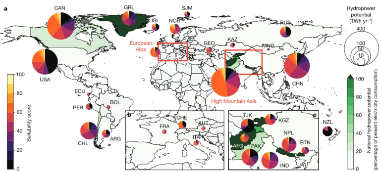
A suitability score higher than 50 (an inflection point in the cumu-lative distribution of the scores; Extended Data Fig. 3a) is achieved by 39% (534 ± 202 TWh yr–1) of the theoretical hydropower potential (Fig. 1a, b; see Extended Data Fig. 3a for any other score threshold). The amount can be put into perspective by aggregating it per country and comparing it with the national energy consumption28
(Fig. 2). The glacier basins of Nepal, Afghanistan, Bhutan and Kyrgyzstan contain enough hydropower potential to exceed present electricity consump-tion, although this is partly due to very low demand per capita. Other countries with large potential include Tajikistan (82% of current con-sumption), Chile (40%), Pakistan (35%) and Georgia (31%). Canada, Iceland, Bolivia, Norway and Switzerland have the potential for 10–23% of their present consumption, and the numbers become even more important when compared with today’s national renewable electric-ity production (Extended Data Fig. 7). Suitabilelectric-ity scores higher than
CAN USA MNG CHN NZL KAZ GEO GRL RUS SJM NOR ISL ECU PER BOL CHL ARG European Alps
High Mountain Asia
400 10 50 100 Hydropower potential (TWh yr–1) 100 80 60 40 20 0 National hydr opower potential (per centage of pr
esent electricity consumption)
100 80 60 40 20 0 Suitability scor e a IND TJK AFG PAK BTN NPL KGZ c FRA CHE AUT ITA b
Fig. 2 | Global distribution of the hydropower potential from deglacierizing areas, showing suitability and national significance. a–c, Countries are coloured according to the nationally aggregated hydropower potential from sites with suitability scores of 50 or more, as a percentage of the present-day national electricity consumption28 (green shading). The pie charts show the
maximal hydropower potential (pie size) broken down by suitability score (pie colours). Countries that are aggregated as European Alps and High Mountain Asia in panel a are magnified in panels b and c, respectively. Colour graduations are discretized for better readability. The basemap was generated using Matplotlib30. Hydr opower potential (TWh yr –1) 10 0 United States (0.3%) China (0.2%) Canada (1.9%) Chile (3.4%) Bhutan (104.3%) Pakistan (6.2%) Nepal (187.7%) Switzerland (2.7%) Tajikistan (13.8 %) Greenland (51.3%) Kyrgyzstan (13.5%) India (0.5%) Afghanistan (36.2%)
Environmental Technical Economic
World HeritageProtected ar ea
Endanger ed species Slope instabilityGlacier sur
ging
Ocean terminatingReservoir infill timeBasin deglacierizationProduction costCombined scor e Suitability scor e 100 0 80 60 40 20
Fig. 3 | Cumulative hydropower potential and average suitability score for the top ten sites per country in terms of total energy potential. Only sites with a suitability score of 50 or more are considered. For each indicated country, the total potential of the largest ten sites is shown by the bar heights. The potentially provided percentage of the national electricity consumption is in parentheses. Colours show the average suitability, grouped into three categories of indicators (labelled at the bottom) and a combined suitability score (see Methods). Only nations with a total potential of more than 1.5 TWh yr–1
are shown. Colour graduations are discretized for better readability. 75 are found for 4% (51 ± 19 TWh yr–1) of the theoretical potential, the
highest potentials being located in Canada (15.6 ± 5.9 TWh yr–1 ), the US (10.7 ± 4.1 TWh yr–1
), China (6.1 ± 2.3 TWh yr–1
), India (4.1 ± 1.6 TWh yr–1 ) and Norway (3.0 ± 1.1 TWh yr–1
).
We emphasize that building a dam at every glacier location is neither realistic, nor sustainable, nor desirable. We find, however, that most of the identified potential comes from a relatively small number of sites. For instance, 1,000 of the roughly 185,000 assessed sites contain 31% (423 ± 160 TWh yr–1) of the total energy potential (Fig. 1b). The global dis-tribution of the sites with the highest energy potential and the relevant suitability scores are given in Extended Data Fig. 8. The ten largest sites with suitability scores larger than 50 could produce 7 TWh yr–1
or more in each of USA, China, Canada and Nepal. That is substantial for Nepal (where this energy potential represents 1.9 times the present electric-ity consumption), but not in China, for example, where this potential pales in comparison with national demand (roughly 5,300 TWh yr–1) and the scale of already-planned hydropower developments18. In Bhu-tan, AfghanisBhu-tan, KyrgyzsBhu-tan, Tajikistan and Greenland, fewer than 10 dams would have the potential to provide more than 10% of national electricity demand (Fig. 3). We note that our estimates consider only the runoff generated within each of the glacierized basins. Although it can be difficult to realize water diversions because of both techni-cal and polititechni-cal constraints, the hydropower potential and the cost efficiency could be substantially increased by diverting water from surrounding basins.
In addition to providing hydropower energy, artificial reservoirs have been suggested to play a role in mitigating changes in seasonal water availability and related water stress6
. As glaciers shrink, so does their ability to store snow and ice over long time periods, and to release the corresponding water during the melt season3. Reservoirs might imitate this storage function, to the benefit of arid regions relying on meltwater during the dry season. The globally aggregated reservoir volume corresponds to 48% of the average annual runoff from the contributing glacier catchments, hinting at the substantial potential for water management in such sites.
Our analyses are a first quantification of the global potential for hydropower production and water storage in deglacierizing areas.
Further assessment of the actual feasibility of the locations identi-fied here would be needed on a case-by-case basis. Particularly impor-tant will be an understanding of the local energy and development
framework, a demonstrated need for additional infrastructure, and a detailed environmental, technical and economic feasibility assessment. Changing glacial environments are an emotive topic exemplifying global change in a very tangible way, and outside interference can be met with apprehension12,29. Accounting for the concerns and needs of local communities and safeguarding the functioning of downstream ecosystems should be of utmost importance when planning for new infrastructure.
Online content
Any methods, additional references, Nature Research reporting sum-maries, source data, extended data, supplementary information, acknowledgements, peer review information; details of author con-tributions and competing interests; and statements of data and code availability are available at https://doi.org/10.1038/s41586-019-1740-z.
1. Vaughan, D. et al. in Climate Change 2013: The Physical Science Basis. Contribution of Working Group I to the Fifth Assessment Report of the Intergovernmental Panel on Climate Change (eds Stocker, T. et al.) 317–382 (Cambridge Univ. Press, 2013).
2. Immerzeel, W. W, van Beek, L. P. H. & Bierkens, M. F. P. Climate change will affect the Asian water towers. Science 328, 1382–1385 (2010).
3. Huss, M. & Hock, R. Global-scale hydrological response to future glacier mass loss. Nat. Clim. Chang. 8, 135–140 (2018).
4. Stoffel, M. & Huggel, C. Effects of climate change on mass movements in mountain environments. Prog. Phys. Geogr. Earth Env. 36, 421–439 (2012).
5. Huss, M. & Hock, R. A new model for global glacier change and sea-level rise. Front. Earth Sci. 3, 54 (2015).
6. Farinotti, D., Pistocchi, A. & Huss, M. From dwindling ice to headwater lakes: could dams replace glaciers in the European Alps? Environ. Res. Lett. 11, 054022 (2016).
7. Marzeion, B., Kaser, G., Maussion, F. & Champollion, N. Limited influence of climate change mitigation on short-term glacier mass loss. Nat. Clim. Chang. 8, 305–308 (2018). 8. Hock, R. et al. GlacierMIP—a model intercomparison of global-scale glacier
mass-balance models and projections. J. Glaciol. 65, 453–467 (2019).
9. Church, J. et al. in Climate Change 2013: The Physical Science Basis. Contribution of Working Group I to the Fifth Assessment Report of the Intergovernmental Panel on Climate Change (eds Stocker, T. et al.) 1137–1216 (Cambridge Univ. Press, 2013).
10. Terrier, S., Bieri, M., Jordan, F. & Schleiss, A. J. Impact du retrait glaciaire et adaptation du potentiel hydroelectrique dans les Alpes suisses. La Houille Blanche 1, 93–101 (2015).
11. Haeberli, W. et al. New lakes in deglaciating high-mountain regions—opportunities and risks. Clim. Change 139, 201–214 (2016).
12. Colonia, D. et al. Compiling an inventory of glacier-bed overdeepenings and potential new lakes in de-glaciating areas of the Peruvian Andes: approach, first results, and perspectives for adaptation to climate change. Water 9, 336 (2017).
13. Best, J. Anthropogenic stresses on the world’s big rivers. Nat. Geosci. 12, 7–21 (2019). 14. Pritchard, H. D. Asia’s shrinking glaciers protect large populations from drought stress.
Nature 569, 649–654 (2019).
15. Kraftwerke Obserhasli AG. Speichersee und Kraftwerk Trift. https://www.grimselstrom.ch/
ausbauvorhaben/zukunft/kraftwerk-trift/ (accessed June 2019).
16. International Renewable Energy Agency. Installed renewable energy capacity. http://
resourceirena.irena.org/gateway/dashboard/?topic=4&subTopic=16 (2018).
17. Nemergut, D. et al. Microbial community succession in an unvegetated, recently deglaciated soil. Microb. Ecol. 53, 110–122 (2007).
18. Zarfl, C., Lumsdon, A., Berlekamp, J., Tydecks, L. & Tockner, K. A global boom in hydropower dam construction. Aquat. Sci. 77, 161–170 (2015).
19. Latrubesse, E. et al. Damming the rivers of the Amazon basin. Nature 546, 363–369 (2017).
20. RGI Consortium. Randolph Glacier Inventory—a dataset of global glacier outlines, version 6.0. Technical Report (Global Land Ice Measurements from Space (GLIMS), 2017). 21. Gernaat, D. E. H. J., Bogaart, P. W., van Vuuren, D. P., Biemans, H. & Niessink, R.
High-resolution assessment of global technical and economic hydropower potential. Nat. Energy 2, 821–828 (2017).
22. Huss, M. & Farinotti, D. Distributed ice thickness and volume of all glaciers around the globe. J. Geophys. Res. 117, F04010 (2012).
23. van Vuuren, D. P. et al. The representative concentration pathways: an overview. Clim. Change 109, 5–31 (2011).
24. International Hydropower Association. Hydropower Sustainability Assessment Protocol Technical Report (International Hydropower Association, 2012).
25. Chao, B., Wu, Y. H. & Li, Y. S. Impact of artificial reservoir water impoundment on global sea level. Science 320, 212–214 (2008).
26. International Energy Agency (IEA). Key world energy statistics report 2017. https://www.
iea.org/publications/freepublications/publication/KeyWorld2017.pdf (2017).
27. Bosson, J.-B., Huss, M. & Osipova, E. Disappearing World Heritage glaciers as a keystone of nature conservation in a changing climate. Earth's Future 7, 469–479 (2019). 28. The World Bank World development indicators 2018. https://datacatalog.worldbank.org/
dataset/world-development-indicators (2018).
29. Byg, A. & Salick, J. Local perspectives on a global phenomenon—climate change in Eastern Tibetan villages. Glob. Environ. Change 19, 156–166 (2009).
30. Hunter, J. D. Matplotlib: a 2D graphics environment. Comput. Sci. Eng. 9, 90–95 (2007).
Methods
We apply the methods and suitability assessments described below to each individual glacier in the globally complete Randolph Glacier Inventory20 (RGI, version 6), excluding the Sub-Antarctic and glaciers smaller than 0.05 km2
. Each of the 187,268 glaciers is considered to be a separate potential site. The lowest point of the glacierized area—the terminus—is set as the potential dam-wall location and watershed-collection point, limiting our study to areas that are ice-covered at present (years 2002 ± 10, as given by the glacier inventory).
Potential storage capacity
Digital elevation models (DEMs) of the subglacial topography of each loca-tion are determined by subtracting the estimated ice thickness (derived from the global ice-thickness model of ref. 22
) from DEMs of the glacier surface31,32
. Dam walls are simulated at the lowest point of each glacier to determine the potential reservoir volume in the future ice-free area. The walls are simulated to be perpendicular to the glacier centre lines33, and at rotations of ± 15° and ± 30°. The orientation returning the largest ratio of reservoir volume to dam-wall area is selected. Dams are grown to the maxi-mum volume that can be accommodated by the local ice-free topography, with wall dimensions limited to 800 m in width and 280 m in height to reflect the maximum dimensions of existing dams in high-mountain areas.
For each site, we calculate the uncertainty in simulated storage vol-ume through the uncertainty in ice thickness from which subglacial topography is inferred. The latter has been assessed to be of the order of 20% at the point scale and 30% for the glacier-wide scale34. Note that this uncertainty does not affect the estimated hydropower potential, as the storage volume does not enter those computations (see below). By comparison with a manual or a more sophisticated dam-wall placement that further optimizes the location within the valley topography, our simulation provides a conservative estimate for reservoir volumes. Hydropower potential
The potential hydropower production over a certain time period, Et (in watt-hours, Wh), is primarily a function of water availability, available hydraulic head and system design:
∑
Et= min(Q Q, )Δthρgη (1)
t t D
where Qt and QD are the discharge rate and the design discharge rate (in m3
s–1
), respectively; ∆t is the time step (in hours); h is the available hydraulic head (in m); ρg is the specific weight of water (9,800 N m–3
); and η is the system efficiency (dimensionless, conservatively estimated as 80%; ref. 21
). Qt is modelled at a monthly resolution (see below), while QD is defined as the minimum discharge that is required to turbine the entire basin runoff every year. For sites with no reservoir, QD is the maximal monthly discharge. For sites with a reservoir, QD is instead the maximum between the average monthly discharge and the discharge level that, if exceeded, results in a water volume that is equal to the vol-ume of the reservoir (Extended Data Fig. 9). When considering annual electricity production, this definition of QD allows us to replace min(Qt, QD) in equation (1) with the average annual discharge.
The catchment from which runoff is generated is defined by applying a watershed delineation algorithm35 to the DEM of the subglacial topogra-phy and the surrounding non-glacierized catchment area. Projections of specific runoff rates at monthly resolution come from the Global Glacier Evolution Model (GloGEM)5
. GloGEM is a state-of-the-art glacier evolution model that computes glacier mass balance and glacier geometry changes for each individual glacier. The glacierized portion of each catchment has an annually updated geometry (area and elevation distribution), and basin runoff consists of rain and melt (from snow, firn and ice), minus refreez-ing. Processes such as groundwater recharge or evapotranspiration are not explicitly accounted for, because there is a lack of data to constrain the processes at the considered scale, and because their contribution is
expected to be small in the addressed, highly glacierized catchments. GloGEM is driven by climate projections from 14 global climate models (GCMs)36, which in turn account for three future greenhouse gas concen-tration pathways23: RCP 2.6, 4.5 and 8.5. Annual average discharge rates are computed by averaging over the 14 GCMs and all months of the year. The presented values for hydropower potential are averages over the years 2020–2100 and all three emission scenarios.
The available hydraulic head over which hydropower could be pro-duced is determined for each site as the maximum topographic drop from the base of the simulated dam wall to a maximum distance of 2, 4, 6, 8, 10, 12 and 15 km. Topographic drops are determined using the 3-arc-second Viewfinder Panoramas global DEM37,38. The range of distances over which the hydraulic head is calculated provides possible energy-production options for each site. For each option we estimate a produc-tion cost (see ‘Economic indicators’ below), and we choose the opproduc-tion with the lowest cost per unit of produced energy. We use the standard deviation of the hydraulic heads calculated with the various options (16% on average) as an estimate of the corresponding uncertainty.
The uncertainty in total energy potential, averaged over all climate models, all emissions scenarios, and all years from 2020–2100, is esti-mated as ± 33%. The individual uncertainty components, combined in quadrature, stem from the estimated hydraulic head (± 16%), the 14 dif-ferent climate models (± 20%), the three emissions scenarios (± 12%), and temporal variation over the considered period (± 17%). We assume that all runoff is available for energy production but neglect the possibility of diverting water from beyond the watershed. Note that calculations of potential hydropower production are independent of the potential dam volume assessments (the dam volume does not feature in equation (1)). Sites with a topography that is unfavourable for dam construction can therefore be thought of as run-on-river power plants. Such a lack of storage capacity, however, is penalized in the suitability score. Suitability score
We rate the suitability of each potential site with a score ranging from 0 (unsuited) to 100 (highly suited). The score is the average value assigned to three equally weighted categories that account for environmental, technical and economic factors. The individual categories comprise between one and five independently rated indicators (again with a value between 0 and 100), and the value of the worst-scoring indicator is con-servatively assigned to the corresponding category. Some indicators are treated as ‘killer’ criteria, meaning that if a given criterion is met, an overall suitability score of 0 is assigned irrespective of any other indica-tor. Details for the computation of individual indicator are given below. Environmental indicators. Environmental indicators include: (1) the presence of UNESCO World Heritage Sites (retrieved from ref. 39
); (2) the presence of otherwise protected areas (taken from the World Database on Protected Areas (WDPA)40
); and (3) the density of endangered spe-cies (obtained from the Global Amphibian and Mammal Spespe-cies Rich-ness Grids of the International Union for Conservation of Nature41,42). Species-richness grids are available with 30-arc-second resolution, and vector data for UNESCO and protected areas are gridded to the same resolution. Information for every potential site is obtained by intersecting the so-obtained grids with the position of the glacier termi-nus. The scores for the three indicators are assigned as follows: 0 (100) if a location is (is not) within an UNESCO area; 0 (50) if a location is rated as category I (category II) in the WDPA; and 100 if it is rated as category III or is not classified; ‘100 – 10N’ for the density of endangered species, N being the number of such species (score = 0 for N ≥ 10). UNESCO and WDPA category I status are treated as killer criteria.
Technical indicators. Technical indicators include: (1) the reservoir in-fill time; (2) the risk of slope instabilities; (3) the timing by which a given reservoir is projected to become ice-free; (4) the risk of rapid glacier advance (surging); and (5) the presence of an ocean-terminating glacier.
Reservoir infill time—calculated as the ratio between the potential dam volume and the projected annual inflow—is a widely used metric in hydropower engineering. Dams with large infill times are favourable because they have larger potential for storage and water-management purposes, and longer lifespan in terms of sediment infill. A score of 100 is assigned for infill times of more than 6 months, and the score decreases linearly to 0 for zero infill time. The latter also occurs when the reservoir volume is zero—that is, when no suitable dam can be simu-lated within the imposed dimension limits (a common occurrence when the subglacial topography is very wide, very flat or very steep).
We roughly assess the risk of slope instabilities from the 80th percen-tile of a basin’s slope (a metric identifying very steep parts of the basin). The likelihood of high-alpine slope instabilities increases substantially when the slope is steeper than 40° (ref. 43
). A linear score is assigned in the slope range 40 ± 10°, with scores of 0 and 100 assigned to basins with slopes above 50° and below 30°, respectively. Earthquake risk is accounted for in the calculations of production costs (see below).
The timing by which a given reservoir becomes ice-free—which is central to the concept of using currently glacierized areas as potential reservoir locations—is assessed through the GloGEM results (see above). More specifically, the timing is determined as the year by which the lowest glacier elevation rises above the elevation of the simulated dam crest. The most conservative estimate from the three climate scenarios (latest retreat) is used. A score of 0 (or 100) is assigned if the reservoir remains ice-covered until 2100 (or 2040), with a linear score in between. Surging and ocean-terminating glaciers impose risks on the potential infrastructure from rapid glacier advance and ocean waves, respec-tively. Surging glaciers are identified through a recent inventory44, while ocean-terminating glaciers are determined from the elevation of their terminus. Both indicators are binary (with a score of either 0 or 100) and are treated as killer criteria. Note, moreover, that ocean-terminating sites bear only minimal hydropower potential, as their hydraulic head is limited to a fraction of the potential dam height.
Economic indicators. Economic indicators consider only the cost of hydropower production. The calculations are based on the levelized cost of electricity (LCOE)45, which we compute as in ref. 21. This reference uses cost-estimation formulae (see Extended Data Table 1 for details) developed by the Norwegian and US hydropower industries to estimate electricity production costs in early project phases46,47
, and annualizes the investments using a discount rate of 10% over a 40-year economic lifespan. The individual cost components include turbine, piping and power-station costs; costs for electro-technical equipment, power-line connection and site operation; and costs deriving from seismic hazard mitigation, land loss and possible population displacement. The compo-nents are mainly a function of: the installed turbine capacity, PT, which we impose to be large enough to accommodate the entire, theoretically possible production at each site; the design discharge, QD (see above); and geometrical parameters such as dam height, DH, dam length, DL, hydraulic head, h, and length of piping, Lp, which are all given by our topographical analysis. Details on the calculations of the individual cost contributions are given in Extended Data Table 1, while Fig. 1c and Ex-tended Data Fig. 6 provide overviews of the cost distribution. Following the price thresholds used in ref. 21
, we assign a score of 0 (or 100) for sites with production costs above 0.5 USD kWh–1
(or below 0.1 USD kWh–1 ), and we linearly interpolate the score in between. Note that the produc-tion costs are driven largely by the technical infrastructure, and that no distinction is made between price levels in different countries, because most components can be considered to be commodities.
Data availability
The data generated herein are available at http://doi.org/10.3929/ethz-b-000353109. The reference list provides information on data obtained from third parties.
Code availability
The computer codes used for evaluations are available from the cor-responding author upon request.
31. Jarvis, J., Guevara, E., Reuter, H. I. & Nelson, A. D. Hole-filled SRTM for the globe:
version 4: data grid http://srtm.csi.cgiar.org/ (CGIAR Consortium for Spatial
Information, 2008).
32. Tachikawa, T., Hato, M., Kaku, M. & Iwasaki, A. Characteristics of ASTER GDEM version 2. In Proc. IEEE Int. Geosci. Remote Sensing Symp. (IGARSS) 3657–3660 (IEEE, 2011). 33. Machguth, H. & Huss, M. The length of the world’s glaciers—a new approach for the
global calculation of center lines. Cryosphere 8, 1741–1755 (2014).
34. Farinotti, D. et al. How accurate are estimates of glacier ice thickness? Results from ITMIX, the Ice Thickness Models Intercomparison eXperiment. Cryosphere 11, 949–970 (2017).
35. Jenson, S. & Domingue, J. Extracting topographic structure from digital elevation data for geographic information-system analysis. Photogramm. Eng. Remote Sensing 54, 1593– 1600 (1988).
36. Taylor, K., Stouffer, R. & Meehl, G. An overview of CMIP5 and the experiment design. Bull. Am. Meteorol. Soc. 93, 485–498 (2012).
37. Lloyd, C., Sorichetta, A. & Tatem, A. High resolution global gridded data for use in population studies. Sci. Data 4, 170001 (2017).
38. de Ferranti, J. Digital Elevation Data http://www.viewfinderPanoramas.org/dem3.html
(2014).
39. International Union for Conservation of Nature (IUCN) and UNEP-WCMC. KML layer of natural and mixed world heritage sites as recorded in the World Database on Protected
Areas (WDPA). http://www.iucn.org/sites/dev/files/import/downloads/natural_and_mixed_
world_heritage_sites_2014.kmz (2013).
40. International Union for Conservation of Nature (IUCN) and UNEP-WCMC. The World
Database on Protected Areas (WDPA). Protected Planet https://www.protectedplanet.
net/ (2017).
41. International Union for Conservation of Nature (IUCN) and Center for International Earth Science Information Network. Gridded species distribution: global amphibian richness
grids.
https://sedac.ciesin.columbia.edu/data/set/species-global-amphibian-richness-2015 (NASA Socioeconomic Data and Applications Center (SEDAC), 2015).
42. International Union for Conservation of Nature (IUCN) and Center for International Earth Science Information Network. Gridded species distribution: global mammal richness
grids.
http://sedac.ciesin.columbia.edu/data/set/species-global-mammal-richness-2015(NASA Socioeconomic Data and Applications Center (SEDAC), 2015). 43. Fischer, L., Purves, R., Huggel, C., Noetzli, J. & Haeberli, W. On the influence of
topographic, geological and cryospheric factors on rock avalanches and rockfalls in high-mountain areas. Natural Hazards Earth Syst. Sci. 12, 241–254 (2012).
44. Sevestre, H. & Benn, D. Climatic and geometric controls on the global distribution of surge-type glaciers: implications for a unifying model of surging. J. Glaciol. 61, 646–662 (2015).
45. International Renewable Energy Agency. Renewable energy technologies: cost analysis
series Vol. 1 Power Sector Issue 3/5 https://www.academia.edu/12663204/renewable_
energy_technologies_cost_analysis_series (IREA, 2012).
46. SWECO Norge AS. Cost base for hydropower plants (with a generating capacity of more
than 10,000 kW). http://publikasjoner.nve.no/veileder/2012/veileder2012_03.pdf
(Norwegian Water Resources and Energy Directorate, 2012).
47. Hall, D., Hunt, R., Reeves, K. & Carroll, G. Parameters of US Hydropower Resources. Contract No. INEEL/EXT-03-00662. Technical Report (Idaho National Engineering and Environmental Laboratory, 2003).
48. SWECO Norge AS. Cost base for small-scale hydropower plants (with a generating
capacity of up to 10,000 kW). http://publikasjoner.nve.no/veileder/2012/veileder2012_02.
pdf (Norwegian Water Resources and Energy Directorate, 2012).
49. Giardini, D., Grünthal, G., Shedlock, K. M. & Zhang, P. The GSHAP global seismic hazard map. Ann. Geophys. 42, 1225–1230 (1999).
50. Harris, J., Bonneville, D., Kersting, R. A., Lawson, J. & Morris, P. Cost Analyses and Benefit Studies for Earthquake-Resistant Construction in Memphis, Tennessee—Design Drawings. Report No. 14-917-26,
https://www.nist.gov/publications/cost-analyses-and-benefit-studies-earthquake-resistant-construction-memphis-tennessee-0. (NIST, 2013
51. Food and Agriculture Organization of the United Nations. FAOSTAT Annual producer
prices 2015. http://www.fao.org/prices/en/#data/PP (2015).
Acknowledgements This study was supported by the Swiss National Science Foundation
(SNSF), grant number PZENP2_154290. We thank all those who made freely available any data used here; D. Gernaat for distance-to-powerline information used in the economic analysis; and D. Felix for punctual advice regarding hydropower infrastructure design.
Author contributions D.F. and V.R. conceived the study; M.H. produced the glacier runoff
projections and provided the DEMs necessary for the analyses; D.F. conceived and implemented the code for the dam-construction analysis; V.R. conceived the suitability score system with the help of D.F. and H.Z.; V.R. performed global-scale calculations, and designed most figures; H.Z. and L.C. implemented and performed the economic analyses with the help of D.F., and assisted in figure design and production. The manuscript was drafted by V.R. and D.F., with contributions from M.H., H.Z. and L.C.
Competing interests The authors declare no competing interests. Additional information
Correspondence and requests for materials should be addressed to D.F.
Peer review information Nature thanks Joseph Shea and the other, anonymous, reviewer(s) for
their contribution to the peer review of this work.
Reprints and permissions information is available at http://www.nature.com/reprints.
Extended Data Fig. 1 | Visualization of virtually installed dams and reservoirs. a–f, An arbitrary subset of dams and reservoirs for locations in: a, Alaska; b, Scandinavia; c, North Asia; d, Central Asia; e, Low Latitudes; and f, New Zealand (see Extended Data Fig. 7 for the nomenclature of regions). The
approximate locations of the sites are shown in the bottom right corners. Background images are from GoogleEarth (providers: a–f, DigitalGlobe; b, c, e, Landsat/Copernicus; b, d, e, CNES/Aribus; a, f, Maxar Technologies; f, Planet.com).
Extended Data Fig. 2 | Temporal evolution of the total hydropower potential from all considered basins within individual regions. Regional definitions for panels a–r are in Extended Data Fig. 7 and follow the Randolph Glacier Inventory20. Projections refer to three climate scenarios (green, blue and red)
based on selected representative concentration pathways23. Temporal
variations reflect variations in runoff. Note that different vertical scales are used for each row. Grey shading indicates 95% confidence intervals.
Extended Data Fig. 3 | Cumulative hydropower potential and potential reservoir volume for a given suitability score. a, b, Hydropower potential (a) and reservoir volume (b). The ‘steps’ in the suitability score are caused by some of the suitability indicators only taking discrete values, and the final suitability
score being an average of three categories (see Methods). The inflection point at score 50 is marked, as are other features worth noticing. The suitability score is dimensionless.
Extended Data Fig. 4 | Globally aggregated hydropower potential and potential storage volume as a function of suitability. a, b, Hydropower potential (a) and reservoir volume (b). The score for every suitability indicator
(environmental, technical or economic) is given individually. The last row of each panel shows the final suitability score (see Methods).
Extended Data Fig. 5 | Hydropower potential as a function of suitability, aggregated per country. a–o, The 15 countries with the highest cumulative hydropower potentials. Scores for individual indicators are given separately.
Extended Data Fig. 6 | Cumulative hydropower energy potential as a function of production cost in different regions of the world. a–r, Regions are defined in Extended Data Fig. 7, and are sorted according to the maximal potential for which the estimated production cost is below 0.5 USD kWh–1.
Different colours depict individual cost components (see Methods and Extended Data Table 1 for calculations). Note that the panels have different scales (the grey bars in the upper right corners are always equivalent to 3 TWh yr–1).
Extended Data Fig. 7 | Global distribution of the hydropower potential from deglacierizing basins, compared with present renewable electricity production. The total maximal potential per country (blue shading) is shown as a percentage of the present renewable electricity production. Data for the
latter are taken from the International Renewable Energy Agency16 for the year
2017. The red boxes indicate regions as defined in the Randolph Glacier Inventory20 and are used for aggregating data in Extended Data Figs. 2, 6. The
basemap was generated using Matplotlib30.
Extended Data Fig. 8 | Global distribution of the top 1,000 sites in terms of hydropower potential. Circle sizes and colours depict the hydropower potential and the suitability score, respectively. The basemap was generated using Matplotlib30.
Extended Data Fig. 9 | Conceptual representation of the procedure used for determining the design discharge QD. Qavg is the average monthly discharge
and Vres (orange area) is the volume of the reservoir. Small and large reservoirs
are discerned on the basis of annual discharge: a reservoir is considered to be large if it can store half of the annual discharge or more. In this case, turbining
the annual discharge every year requires QD to equal Qavg (a smaller QD would
imply water accumulation from year to year, thus leading to reservoir overspill and production loss over time). Smaller reservoirs require a larger QD, because
less water can temporarily be stored. Letters on the x-axis denote months.
Extended Data Table 1 | Equations used to compute hydropower production costs
Hydropower production costs are taken as the levelized cost of electricity (LCOE). The calculations of individual cost components pi follow ref. 21. Costs are in 2010 US Dollars (USD). 1 NOK is
approximately 0.12 USD. Equations are from refs. 45,48–51.