Investigation of "Whole Tree" combustion in a packed-bed

(1)

Investigation of "Whole Tree" Combustion in a

Packed-Bed.

by

ABDOULAYEOUEDRAOGO

A dissertation submitted to the Graduate Faculty of North Carolina State University

in partial fulfillment of the requirements for the Degree of

Doctor of Philosophy

Department of Mechanical and Aerospace Engineering

Raleigh 1994

APPROVED By:

-:>

Y1

AJ{..""'3jij~~

Dr. J. M. Anthony DanbY

U

~,~~

rl~0

Dr. R. R. Johnson Dr. M. N. Ozisik Coff'hair of Advis

(2)

DEDICATION

This work is dedicated to

my

wife, ZOURATA OUEDRAOGO and son CHECK ABBAS TEWENDE for their love and understanding.

(3)

BIOGRAPHY

MI. A. OUEDRAOGO holds a Licence de Physique (1977) de l'Universite Chech Anta Diop de DAKAR (west Africa), a Maitrise de Recherche es Sciences Physiques Appli-quees (1978) and a Diplome D'Etudes Approfondies (D.E.A.) D'Energie Solaire (1980) from the same University. Prior to joining (1987) the Institut de Mathematique et Phy-sique now the Faculte des Sciences et Techniques de l'Universite de OUAGADOU-GOU (west Africa), Mr. A. OUEDRAOGO has work as managing officer for SOLAR POMPS (6 units of 1 KW Rankine Cycle type Pomps, known as Thennodymanics pomps and 1 Photovoltaic Pomp of 4.5 KW) and latter earned (1986) a Master of Sci-ence in Mechanical Engineering Degree from the Department of Mechanical Engineer-ing of the University of TUSKEGEE (U.S.A.) where he has investigated the use of bio-fuels in fann equipments.

(4)

ACKNOWLEDGEMENTS

The author wishes to express his deepest appreciation and thanks to Dr. James C.

Mulligan and Dr. John G. Cleland, Co-chairmen of his advisory committee, who have given their time generously in guiding and reviewing all the work.

The author wishes to thank Dr. M. N. Ozisik for exposing him to many new topics and for serving in his advisory committee.

The author also wishes to thank Dr. R. R. Johnson for fruitful discussions and for serving on his advisory committee.

The author also wishes to thank Dr. J. M. Anthony Danby for serving on his advisory committee.

The author wouId gratefully like to acknowledge the financial support and encourage-ment of the African-American Institute through the AFGRAD Fel,lowship.

Finally, the author wishes to thank his Parents and Parents-in-Iaw for their under-standing and encouragement, Idrissa Ouedraogo and Ron E. Burke for their constant support.

(5)

l

t

1

r

t

1

1 (

1

1 r

1

TABLE OF CONTENTS Page LIST OF FIGURES... ix

LIST OF TABLES... XlI

1. A quasi-steady shrinking core analysis of wood

combustion

lolo • • • lolo lolo. • • • • • • • • • • • • • • • • • • • • •

1

1.1 Abstract... 2

1.2 Introduction... 2

1.3 Shrinking core model... 5

1.3.1 Equations of the shrinking core model... 6

1.4 Modeling of the mass transfer coefficient and char layer thickness... 9

1.4.1 Modeling of the mass transfer coefficient... 9

1.4.2 Modeling of the char layer thickness : ;.:... Il 1.5 Model validation... 13

1.6 Conclusion... 15

1.7 References... 31

(6)

1

1 r

1

1 r

1.8 Nomenclature. 32 1.9 Appendix... 33

1.9.1 Code for a single fuel element combustion model... 34

2. A quasi-steady state shrinking core model of

"whole tree" combustion in a countercurrent

fixed-bed reactor...

43

2.1 Abstract... 44

2.3 Mode1 development... 46

2.3.1 Buming rate submodel... 46

2.3.2 Conservation equations in the solid phase... 49

2.3.3 Conservation equations in the gas phase... 51

2.4 Results and discussion... 53

2.7 Nomenclature... 79

2.8 Appendix :... 82

2.8.1 Code for the quasi-steady model... 83

(7)

1

1 !

1

r

1

1 J

1

1 [

1

1 r

J

r

3. Transient moving boundary shrinking core model

of "whole tree" combustion in a countercurrent

fixed-bed reactor...

91

3.1 Abstract... 91

3.3 Upper region modeling: Preheat submodel... 94

3.4 Solid phase combustion... 97

3.4.1 Shell combustion submodel... 97

3.4.2 Core drying and pyrolysis submodel... 99

3.4.3 Core-shell interface modeling... 100

3.5 Gas phase combustion... 100

3.6 Numerical method : Finite Difference Approximation... 101

3.6.1 Internai nodes... 102

3.6.2 Convective boundary nodes... 104

3.6.3 Centerline nodes... 104

3.6.4 Interface nodes... 105

3.6.5 Determination of the time step... 105

3.6.6 Bed spatial grid... 106

3.7 Continuous Mapping Variable Grid Method :CMVGM... 106

3.8 Results and discussion... 110

3.8.1 Preheatprofile... 110

3.8.2 CMVGM solution of the combustion model... 111

(8)

1

1 r

1

1 [

(

r

[

!

l

1

Fig. 2.6

r

l

r

LIST OF FIGURES Page

Fuel element mode!... 17

Energy balance at the char surface... 18

Energy balance at the core surface... 18

Fractional mass loss... 19

Normalized radial shrinking rate... 20

Bumout time of 10 mm cubic particles... 21

Variation ofbumout time with radius ,... 22

Effect of moisture on bumout time... 23

Bumout time of small particles... 24

Moisture effect on average shrinking rate... 25

Char layer thickness of small particles... 26

Char layer thickness of 10 cm long chunkwood... 27

Surface temperature of 10 cm long chunkwood... 28

Surface temperature of 10 cm long chunkwood, a =72%... 29

Effect of moisture on particles bumout time... 30

"Whole tree" bum fuel conversion sequence... 58

"Whole tree" bum power plant... 59

Fuel cel!. ....·;... 49

Moisture effect on residence time... 60

Effect of fuel elements size on residence time... 61

Moisture effect on combustion zone depth.... 62

(10)

1

1 r

1 (

1

1 [

1 r

(

f

1 r

[

r

Fig. 2.7 Fig. 2.8 Fig. 2.9 Fig. 2.10 Fig. 2.11 Fig. 2.12 Fig. 2.13 Fig. 2.14 Fig. 2.15 Fig. 2.16 Fig. 2.17 Fig. 2.18 Fig. 2.19 Fig. 2.20 Fig. 2.21 Fig. 3.1 Fig. 3.2 Fig. 3.3 Fig. 3.4 Fig. 3.5 Fig. 3.6 Fig. 3.7

Effect of fuel elements size on combustion zone depth... 63

Residence time of small particles... 64

Combustion zone depth of small particles... 65

Moisture effect on average shrinking rate... 66

=80%. mc = 50%... 72

Surface and gas temperatures, R_o= 0.1016 m, a =100%,

r

=80% mc = 60%... 73

Oxygen concentration... 74

Normalized radial shrinking rate... 75

Effect of superficial gas velocity on residence time... 76

Effect of superficial gas velocity on combustion zone depth... 77

Interface and nearest core and shell nodes... 119

Computational domain : Variable fuel and bed grids... 120

Preheat profiles. Ro = 0.1016 m, mc = 33.3 %... 121

Preheat profiles. Ro = 0.2540 m, mc = 33.3 %... 122

Core and shell temperature profiles. Ro = 0.1016 m... 123

Core and shell temperature profiles. Ro = 0.2540 m... 124

Selected temperature profiles, Ro = 0.1016 m... 125

(11)

1

1 [

1 r

1 (

1 t

1

1 r

Fig. 3.8 Selected temperature profiles, Ro=0.2540 m... 126

(12)

1

1 r

t

r

Table 1.1 Table 2.1 Table 2.2 Table 3.1 Table 3.2 Table 3.3 Table 3.4 Table 3.5 LIST OF TABLES

Constant thermal properties .

Characteristics of the bed ..

Constant thermal properties .

Bed depth of the two models ..

Bumout time of the two models ..

Oxygen concentration and preheated gas temperature at the

A shrinking core model of the combustion of individual chunkwood and particle wood· elements is developed and validated by comparison with literature data. The model is fonnulated on the physical evidence that large wood specimens inserted into a hot environment lose weight mostly over a relatively thin outside layer, while the inte-rior (core) remains relatively undisturhed. The modeling of the complete process re-quires a correlation of the turbulent heat and mass transfer coefficients which includes the effects of transpiration of volatilized organic compounds and moisture, geometry, and shrinking radius. The fuel element bumout time is shown to he a function of fuel properties, moisture content and size. Drier and smaller elements bum faster while mois-ture is shown to slow the shrinking rate due to the cooling effects of transpiration and the latent heat of evaporation.

1.2 Introduction

Barly analysis of wood decomposition and combustion were almost entirely con-cemed with pyrolysis reactions and the kinetics of small water-free samples hecause of the lack of data in these areas. The physics and heat transfer aspects were usually lumped into an apparent activation energy and frequency factor, and the entire decompo-sition process modeled following a first-order Arrhenius reaction. The temperature was obtained by solving the classical heat conduction equation with the heat of reaction as a source tenn. This approach, however, has been proven in recent years to he an oversim-plification of the sequence of processes which actually occur, particularly for large sam-pIes. As the extemal surface of wood is exposed to a heat flux, the solid heats up at frrst mostly by transient conduction, although there is evidence of moisture migration and perhaps even convection in this phase. When the surface is hot enough, it starts to pyro-lyze into volatiles and residual char. At a certain stage in the heating process, a network of cracks and fissures develops on the surface and propagates into the wood in associa-tion with the pyrolysis wave. The gases produced in the early pyrolysis flow back through the char layer, which becomes a zone of secondary reactions and heat exchange.

(15)

,

l

1 r

l

[

1 r

[

r

~

t

[

l

[

1

r

!

r

In the unfissured zone, volatile products are somehow trapped, increasing the internal pressure. A portion of the volatiles and moisture are forced toward the interior where va-pors may condense and eventually re-evaporate as the pyrolysis front progresses. The process is seen to be extremely complex and, thetefore, it has become customary to at-tempt to incliJde such effects as transient diffusion and conduction, internal convection, heat generation and radiation energy, along with the Arrhenius decomposition, in the formulation of a burning mode!. Contrary to early formulations, it is now common prac-tice to consider wood pyrolysis and combustion as a heat and mass transfer constrained process, either alone or combined with chemical kinetics. Infact, for large particles con-fined in a hot environment, the reaction rate is so great that the reaction itself is localized at the external surface of the fuel element and mass transfer becomes the rate controlling factor.

Blackshear and Kanury [1.1] used the similarities hetween the burning of cellulosic material inair and the burning of fuel-soaked wicks employing CH₃0H, whose driving force is known, to infer the heat and mass transfer coefficients of a-eellulose cylinders. The mass flux is expressed in diffusion form as the product of the mass transfer coeffi-cient and the driving force. Itwas found that the mass transfer coefficient, which is for-mulated as a product of a constant mass transfer coefficient without blowing and a driv-ing force, is dependent upon the thickness of the pyrolyzdriv-ing solid and time.

Maa and Bailie [1.2] are helieved to he the first to apply the shrinking core model to the description of the pyrolysis of cellulosic material. The pyrolysis is assumed to take place at the surface of an unreacted shrinking core which is surrounded by a layer of ma-terial that has been pyrolyzed. The char in the char layer is assumed to he inert and does not undergo reaction. Hence, the reaction is taken to occur at the interface hetween the two solid regions. It is assumed that the thickness of the pyrolyzing zone is negligible and there is a sharp interface between the unreacted central core and the outer char layer. The unreacted core is modeled following the Arrhenius first-order decomposition tion. The temperature profile is obtained by solving the classical heat conduction equa-tion with the addiequa-tion of the bulk flow term with the shrinking core characteristics.

(16)

1

1 l

r

1 r

[

l

t

1

1 l

Saastamoinen and Richard [1.3] have also used a shrinking core fonnulation and ob-tained a total combustion time as a sum of the combustion time with infinitely fast chemical reaction and the combustion time with infinitely fast diffusion rate. The equa-tion used for the diffusion coefficient is similar to that of Blackshear and Kanury but is expressed in tenns of the mass flux, which is itself a function of the diffusion coefficient. Hence, unless an independent correlation can he found, no apparent closure exists for these relations.

Ragland et al. [1.4] followed a similar concept in modeling chunkwood, although the burning rate fonnulation was based on mass transfer considerations alone. The heat transfer equation used is a replica of the early models. The mass transfer equation was modeled following the evaporation of a single sphere in forced convection, hence is only a function of the fuel radius and flow characteristics. For unspecified reasons, however, the radius was kept constant as the fuel element shrinks, consequently the mass transfer coefficient remains constant for prescribed flow characteristics. The model is reported to predict the experimental findings of a constant shrinking rate of 1.8 mm1min. The burn-ing rate is shown to depend on the chunkwood size but independent of its initial moisture content.

In this paper the shrinking core model is developed further and applied to the case of combustion of chunkwood and particle wood elements. The basic concept of an unre-acted core is well established and assumed here. Additional assumptions will he dis-cussed in the following sections. The present work differs from previous studies in that attention is focused primarily on the following elements:

1) The development of an appropriate mass transfer coefficient and its explicit correla-tion as a funccorrela-tion of the transpiracorrela-tion of volatilized organic compounds and moisture, ge-ometry and shrinking radius.

2) The quantitative evaluation of the fuel element moisture content on the burnout time. 3) The appropriate correlation of the heat transfer coefficient.

(17)

[

1

1 r

1

4) The complete modeling of the shrinking char layer and the possible replacement of the general thermal equations by quasi-steady balance equations at the char and core sur-faces.

The work is divided into three main parts. First, a more complete theoretical basis of the shrinking core model is formulated. Secondly, the char layer thickness and the mass transfer coefficient are correlated using the experimental results of Ragland et al. [1.4] on the combustion of chunkwood and Simmons and Ragland [1.5] on the combustion of small cubes. Third, the results are compared with those of previous investigators.

1.3 Shrinking core model

Experimental observations have shown [1.6] that large cylindricallogs inserted into a hot environment lose weight over a relatively thin outside layer while the interior (core) remains relatively undisturbed. The logs lose weight due to transpiration of volatilized organic compounds and water vapor through their surface, leaving behind a char layer which also shrinks while reacting with oxygen in heterogeneous combustion. The de-composition and combustion of cellulosic material may then be regarded as the superpo-sition of two physical processes. First, the thermal decomposuperpo-sition process, which is re-lated to the accumulation and propagation of heat by conduction and convection. This process occurs with the passage of a pyrolysis wave and results in the internal release of volatiles and water vapor. Second, the combustion process, which consists of heteroge-neous combustion of a surface char layer as weIl as the combustion of gaseous products (volatiles). The heat release then in turn sustains the combustion.

While physical evidence shows that pyrolysis and combustion processes !Jf large po-rous fuel elements occur simultaneously [1.6], many investigators, have formulated models on the assumption of separate and distinct phases. Mukunda et al. [1.7] modeled the combustion of dried wooden spheres assuming two separate regimes. These were first, the flaming regime during which the spheres lose weight exclusively due to the loss of volatiles, followed by a glowing regime describing the surface combustion of porous char. The effects of blowing of volatiles and moisture (transpiration) are usually ignored

(18)

1.3.1 Equations of the shrinking core model

[1.4,1.7], or not explicitly accounted for [1.1-1.3]. The mass transfer coefficient pro-posed by Ragland et al. [104] is in fact a mass transfer coefficient without blowing and while it may be an approximation, it is not adequate in describing the simultaneous proc-ess of decomposition and combustion of cellulosic materials. Likewise, neither Black-shear and Kanury [1.1] nor Saastamoinen and Richard [1.3] explicitly correlated the overall mass transfer coefficient to account for both the effects of transpiration and oxy-gen diffusion. In analyzing the glowing combustion even for fuel particles as small as coal, Yoon et al. [1.8] began speaking of the concept of the three phases of drying, py-rolysis and combustion which, in reality, overlap.

To model the complete process, consider the motionless one dimensional fuel element sitting in a gravity-free environment shown in Figure 1.1 An unreacted shrinking core of radius r_w is surrounded by a char layer of thickness b_e and a gas fIlm. The pyrolysis layer is assumed thin and, for simplicity the secondary reactions eomprising the process of "cooking" and internal pressure build-up are ignored. Also, the heat of reaction of py-rolysis is neglected [1.9]. Because of differences in geometry between the model and tual three dimensional fuel elements, a geometry correction factor K is introduced to ac-count primarily for end and corner effects on the overall transfer coefficients. The model fuel element is conceived from actual fuel elements [lA] of yellow poplar and black spruce wood chunks of 7.5 cm radius and 5, 7.5 and 10 cm length, and 10 mm cubes of sugar pine [1.5]. The conditions of modeling of the heterogeneous combustion have been clearly postulated by Walker, Rusinko and Austin [1.10] in the three-temperature-zone theory. It is assumed in our model, however, that when the fuel elements are inserted into the hot environment, their surface temperature reaches instantly a quasi-steady state condition with the subsequent formation of a char layer. This excludes, of course, the short initial phase of transient warming to ignition.

l

i

[

1

1 r

1 f

1

Following Ragland et al, [lA], the rate of mass loss may be written as

dm 'A'"

- = - l m

dt (1. 1)

(19)

1

where ~is the rate of chernical reaction. Combining equations (1.2) and(l.4) yields Now, if the reaction is taken to be of first-order, Equation (1.3) mayheexplicitly

writ-ten as (1.2) (1.5) (1.3) (l.4) ." Kp hD m

=

K +h Coo P D

Defining the free stream oxygen concentration as C00 and the concentration at the fuel

surface by Cs' the mass flux may be expressed in a form sirnilar to that of Blakshear and Kanury [1.1], as the product of the overall mass transfer coefficient (the oxygen mass transfer coefficient modified by transpiration) and the driving force

where m is the mass of the fuel element, A is the external surface area, l represents the

stoichiometric index and in" is the surface mass flux.

The reaction rate at the surface is a function of the concentration of the oxidizer, which depends itself on the actual kinetics of the mechanism at the surface. Ifwe assume this functional relationship to be of the form f(C_s)' then under stationary conditions, the reac-tion rate at the surface musthe equal to the rate at which the reactant reaches the inter-face by diffusion [1.11]. That is,

In their model, Saastamoinen and Richard [1.3] have computed the burnout time as a function of both the chernical reaction rate and diffusion rate. But if we assume the ki-netic rate to be faster than the diffusion rate [1.12], which implies that ~» h_D or that the process is controlled solely by diffusion, it is seen that

1

1 r

1 f

1 t

(

[

l

r 7

(20)

1

8 (1.6) (1.7) (1.8) (1.9) (1. 10)

im

=

m

_ehar

We then make the approximation that the bumoff of the char layer may weIl offer a good estimate of the total bumout time of the fuel element. That is, we assume that the total mass of the solid that bums represents the fixed carbon, Le.

Thus equation (1.8) is written as

where ris the outside radius and (le the char density. Neglecting the ash layer and

writ-ing the bumwrit-ing rate as a sum of the unreacted core shrinkwrit-ing rate and the diffusion lim-ited char-oxygen surface reaction rate in Figure 1.1, it is seen that

Furthennore, experimental evidence has shown that in a diffusion controlled environ-ment the product of the heterogeneous char combustion is CO, and the conversion of CO to COZ takes place extemally in the gas phase (gas film) [1.11]. The stoichiometric in-dex, defined as the number of grams of fuel that bums with one gram of oxidizer, is then equal to (1Z/16). Finally, equation (1.7) becomes

Substituting equation (1.6) into (1.1) yields

1

1 r

1

1 r

(

r

1

1 r

J

l

(21)

ew = Sg ( 1

+

me)ewater where b

c is the char thickness, rw = r - bc the core radius, and the core density is ex-pressed as [1.13]

where v is the volume of the fuel element. Applying equation (1.10) to the spherical fuel element in Figure 1.1 and expanding and rearranging yields

Sg is the specific density of wood and mc its moisture content (on wet basis) expressed in percent. The solution of these equations requires explicit relationships for the overall mass transfer coefficient and the char layer thickness.

9

(1.12) (1. Il)

dm _ 2tir _ _ b 2drw ]

di - 4II [ec r dt

+

(ew ec)(r c) dt

St 1 - b St_o Rex - eb - 1

As suggested by Blackshear and Kanury [1.1] the external boundary layer thickness and diffusional characteristics are constantly modified by the effects of blowing. Rence, the overall mass transfer coefficient is assumed to have the same fonn as in reference [1.1], wherein experimental results indicated the driving force is a function of the fuel elements size and time. The Reynolds number is assumed sufficiently high so that the mass transfer is turbulent. In an experimental study of the hydrodynamic and heat-transfer behavior of equilibrium and near-equilibrium turbulent boundary layers subject to blowing, Kays and Moffat [1.14] proposed the following correlation to described the effect of blowing:

1.4 Modeling of the mass transfer coefficient

and char layer thickness

1.4.1 Modeling of the mass transfer coefficient

1

1 f

1

1 [

1

1 [

1

1 J

1

(22)

At high Reynolds number, the constant term (Le. 2.) in this equation is negligible.

This relationship is seen to be similar to the mass transfer coefficient in the Ragland ' s model [lA], which is

10 (1.14) (1. 15) (1. 13) b₂

=.

573

me

r0 / r and

*

.425 h_D = 2.06 DReD / 2r h_D = 2.75 K D

Rf;5 /

2r b_l =.766me

r

0 /

r

The heat transfer coefficient is correlated from the mass transfer coefficient as and the mass transfer coefficient without blowing h~ [1.15] is given as where

where St and St are the Stanton number with and without blowing measured at the same o

Reynolds number Rex' b is the blowing parameter. Applying these results to the fuel element in Figure 1.1 and using the experimental results of Simmons and Ragland [1.5] and Ragland et al. [1.4], the overall mass transfer coefficient may be correlated using a relation slightly different from that of Kays and Moffat to account for the physical dif-ferences between the two problems. That is

In equation (1.13), K is a geometry correction factor, D the molecular diffusivity, ReD the Reynolds number, mc the moisture content of the logs, and r_o and r the initial and outside radiL The Schmidt number is taken to be equal to one. For cases of dried fuel elements, the mass transfer coefficient collapses to a corrected value of its no-blowing . counterpart.

1

1 f

1

1 l

r

1

1 J

1

(23)

1

11

1.4.2 Modeling of the char layer thickness

(1. 17) (1. 16) V =_dr dt

v: __

_W _- drw_dt where

A quasi-steady state condition is assumed within the fuel elements. The core tem-perature is taken to be uniform and equal to the ambient temtem-perature. Clearly, this as-sumption is justified during most of the combustion process due to the size of the fuel elements. Itcertainly becomes critical near the end of the combustion, but it is helieved that this will not significantly affect the determination of the bumout time (defined as the time of a given percentage of initial weight loss). This assumption also ensures that the surface temperature remains the only unknown.

An energy balance at the char surface, figure 1.2, labeling V and Vw respectively the regression velocities of the core and char and~ andA their surface areas, yields

where

(Je

is the volumetric heat capacity of air at the gas film temperature. The transpi-ration gases are assumed ideal. We still need an explicit relation for the char layer thick-ness which will he shown to he a function of the surface temperature of the fuel elements and the rate at which the pyrolysis front progresses.

and

Recall that under boundary layer diffusion control, the char goes only to incomplete combustion at the char-gas interface. Also it is known that of all the volatiles released, sometimes only a fraction

a

bum incompletely at the gas-solid interface and the

re-1

1

(24)

1

1 [

1

1 r

1

mainder escapes to the gas phase. Hence, H_as represents the average incomplete heat of combustion of the char and volatiles at the interface.

In equation (1.17), the first tenn on the left represents the total heat released by the combustion, the second tenn is the convected energy between the combustion front and the gas phase, and the third tenn represents the internal convected energy through the char towards the unreacted core. The first and second tenns on the right are respectively the heat transported by thennal conduction away from the combustion zone and the ra-diative exchange between the surface of the solid media and the furnace walls, assuming the flue-gas to be non-participative. Basically the equation expresses the fact that the net heat exchange between the gas and solid phase represents the enthalpy of combustion of the char and volatiles. To keep the fonnulation simple, the existence of thennal equilib-rium between the two phases is assumed.

Now consider the energy balance at the core surface, figure 1.3. The energy entering the core is assumed sufficient enough to heat it up to pyrolysis with the subsequent tran-spiration of organic compounds and moisture due to the phase change of active material to pyrolysis gas (hfg_v) and liquid water to water vapor (hfg_m).

(1. 18)

As it is, equations (1.17) and (1.18) represent a quasi-steady state fonnulation of a mov-ing boundary type problem since the core-char interface changes its position continu-ously due to pyrolysis with the subsequent phase-change of active matters and moisture respectively to volatiles and water vapor. The core being at unifonn temperature throughout, only the surface temperature is unknown. Hence, the problem is a one-phase problem (ablation) sometimes referred to as a "Stefan problem".

Combining equations (1.17) and (1.18) yields the surface temperature T

s. The thennal radiation tenn has been neglected compared to the other thennal quantities. Hence,

(25)

1

13 1.5 Mode! validation

wherej

=

m, c, v. (1.19) (1.20)

Instead of a classical moving boundary type solution, the thin char layer approxima-tion is solved by a simple iterative procedure using the constant thermal properties given in table 1.1 Logs of radius equal to 0.2540 m (10 inches) down to particles of 0.10 mm radius have been tested at various moisture content and selected results are presented. Whenever possible, these results are compared with literature data. AlI the volatiles are assumed to go to incomplete combustion at the char surface (i.e.,

a

=1).

Figure 1.4 shows a plot of the fractional mass loss of 15 cm diameter wood chunks (10 cm long) at 20 and 75 % moisture for both the present model and the model used by Ragland and al. to investigate their experimental data. The bumout time was said to he In their experiments, Ragland et al. [1.4] measured a char layer thickness of 3 mm and 15 mm respectively for green and air-dried chunkwood of 15 cm diameter. For prac-tical purposes then, a solution for a thin char layer approximation may he sufficient. Un-der this assumption, the core and surface recession velocities are assumed to have ap-proximately the same magnitude. However, both this assumption and the uniform core temperature approximation may become critical towards the end of the combustion. We also assume constant thermal properties and negligible radiation transfer.

Now after sorne manipulations in equation (1.18) where Ac is the log-mean area and ne-glecting higher order terms, bc is obtained. It is clearly seen that the char layer thickness is a function of the surface temperature and the core shrinking rate. That is,

1

(26)

1

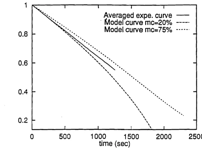
32 min for both values of moisture but this value is shown to fall approximately between the values of our mode!. This is clearly shown in Figure 1.5, where the averaged experi-mental radial shrinking rate is plotted together with our model curve. This averaging process seems to have precluded the observation of any difference between the experi-mental data at the two moistures and may have smoothed out any moisture effect. Rec-ognizing the difficulties of properly accounting for the complete burnout time of the chunkwood after a 30%initial mass loss, the investigators concluded that it appears that moisture has little effect on the rate of combustion at the conditions of these tests. Also by neglecting the blowing effect and keeping the mass transfer coefficient constant in equation (1.9), one would naturally expect to get a constant shrinking rate (1.8 mm1min here) regardless of the initial moisture content of the fuel elements.

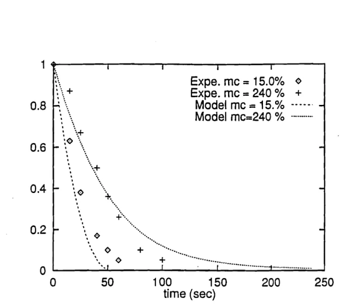
Using additional data, the burnout time of small cubic particle elements of 10 mm size at 15 and 240 % moisture is plotted in Figure 1.6. Here again, the model shows good agreement with the experimental data of Simmons and Ragland [1.5] and it is clearly stated by the authors that the presence of moisture does slow the mass loss rate.If

we let the fuel elements shrink indefinitely or longer than needed, they would seem to have the same burnout time. We should keep in mind, however, that the burnout time is an asymptotic value which for practical purposes should be clearly defined as the time corresponding to a mass loss of 99 %, since it will not make sense on physical grounds to have a solid media whose mass shrinks to zero.

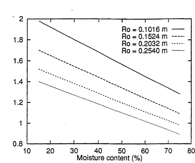
The validated mass transfer coefficient is then used to investigate further the effect of fuel elements size and moisture content on the burnout time tb' As was anticipated, the bumout time is function of the diameter of the logs for a given moisture content, Figure 1.7. It is also shown in Figure 1.8 to be both a function of the fuel element size and moisture content contrary to earlier publications [lA]. The thicker and greener elements take longer to bumout. Also, for a given log the bumout time is not rigorously a simple linear function of its moisture content. As a matter of fact, the bumout time varies from 40 to 60 min for logs of 0.1016 m (4 inches) radius at 15 and 75 % moisture respec-tively, but increases approximately threefold between the same moisture for logs of 0.2540 m (10 inches) radius. Thus, the effects of moisture are more sensible for large size fuel elements than for small ones. It is known that free-water molecules are easily

(27)

l

1 1

1

removed, while bound water molecules in the inner trunks especially when the diameters are large, become harder to remove. These smooth variations become somehow erratic for small samples, Figure 1.9. This was certainly expected and is speculated to 00 caused by both the unifonn core temperature assumption and the thin char layer approximation.

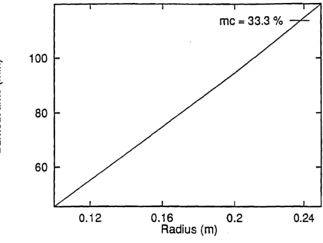
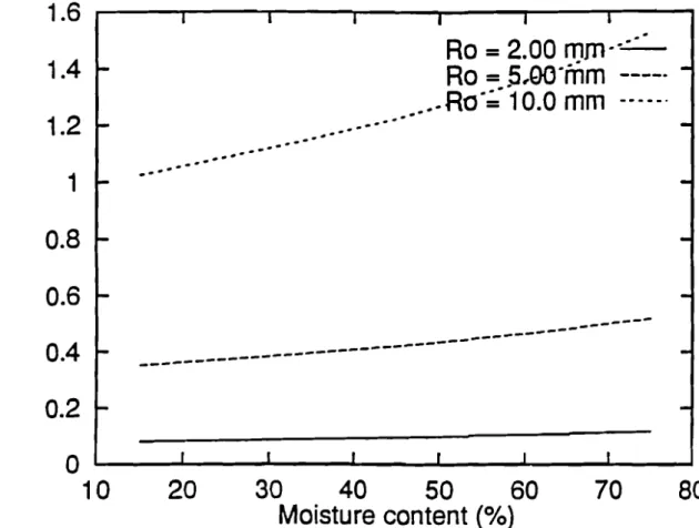
Finally, moisture definitely slows the shrinking rate, which is shown to vary from approximately 2 mm1min at 20 % moisture content to 1.25mm1min at 70 % moisture content for a chunkwood of 0.1016 radius Figure 1.10. As predicted by the model, Fig-ure 1.11 and 1.12 (moistFig-ure content equal33.3 %) show that b

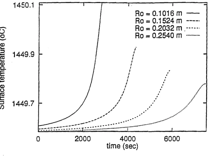
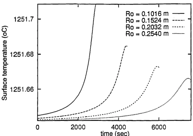
c varies not oruy with the log radius but also shrinks with time while reacting with oxygen. The same oost fit value of 0.60 for K has been used for aIl chunkwood samples, and a slightly lower value of 0.40 for the cubic particles, due to the difference OOtween the two shapes. The surface temperature of the 15 cm diameter chunkwood, Figure 1.13, is quite similar to that found by Ragland et al. [1.4] especially for lower values of

a

(72 %), figure 1.14. The model not only predicts the bumout time of chunkwood and cubic particles but also the bumout time of particles as small as 0.10mmradius. Figure 1.15 shows that it takes about 1 min to combust particles of 10mmradius (the same bumout time approximately is obtained for the 10mmcubic particles in Figure 1.6) while 0.10mmparticles bum instantly.

1.6 Conclusion

The overall mass transfer coefficient correlation in this study is shown to 00 the cen-tral element of the shrinking core mode!. Under boundary layer diffusion control, the ex-ternal boundary layer thickness and diffusional characteristics are constantly modified by the effects of blowing. Hence, for green wood specimens, the cooling effects of transpi-ration of organic compounds and moisture and the latent heat of evapotranspi-ration do slow the burning rate contrary to earlier publications. These chilling effects are found to increase with the amount of moisture content and fuel elements size. The model is simple and yet reliable enough to predict adequately the burnout time of chunkwood and particle fuel elements of different sizes and shapes. Additionally, the model may he used as weIl to investigate the combustion of coal of different sizes and moisture content.

(28)

1

1 _{Table 1.1 Constant thermal properties}

(le ₉₅ _Kg/rn3

_lA

1

Sg

0046

lA

1

T. ₂₅ _Oc 1

1

Tao ₁₂₀₀ Oc

_lA

r

1

16

t

1

(29)

Fig. 1.1 : Fuel element model

1

1 r

1

1 Pyrolysis front

of organic compounds

and water vapor

Volatiles and heterogeneous

char combustion

1200

Oc

25°C:

----...-:.:"':"'".,

..

,

.

,- "

(30)

18

Gas

mm

Transpiration of organic compounds

and water vapor Gas film ,'Interface char-gas " Incomplete

hete-f

rogeneous char " and volatiles ...,' combustion Char layer Char layer r, A, V r, A, V Core

Fig.I.3 : Energy balance at the core surface

Fig. 1.2 :Energy balance at the char surface

Control - volume Interface \ core-char ~ Core Control-volume Interface \ core-char "" ""', " , " , " , , , \, , 1 1 1

1

(31)

Fig. 1.4 : Fractional mass loss

19

-3000

0.4

~

0.6

~

_'.

.

'.

.+ ...

~

.

\"_'. '

.

.. +...

_.

'. ~

.

'. + .

_.

'. ''Q .

'. + ...

' . , A •••••

-v.

+

.

'. <:>

+....

r r -

? ..

~ ~... 1

a

l . -_ _.a..-_ _. . I . . -_ _l-...,;:Q~""~...

=

....

~._~---a

500 1000

1500

2000

2500

time (sec)

41

E

1

(32)

Fig. 1.5 : Normalized radial shrinking rate

Averaged expe. curve

-. Model curve rnc=20

% - - - - .

Model curve rnc=75

% _{._.- •.} 20

2500

2000

1000

1500

..

"

,

"

''''

..

"

'

_'.

"

_"

,

_.

"

_"

'.

_'

"

" _,

"

_"

'.

_.

"

'_'.

"

" _,

"

_"

'.

.

"

_"

" " \

.

\ '. \

'.

\ \

"

\ \ \

500

1

0.8

1

0.6

otl '

-1

1

0.4

1

0.2

1

0

1

(33)

Fig. 1.6 : Burnout time of

10 mm

cubie partieles

21

-250

200

100

150 time (sec)

50

1 ...----.r---...,...---r-.---""'T.----,

Expe. mc

=

15.0%

<)

Expe. mc = 240

%

+

Model mc

=

15.%

._ ..

-Model mc=240

% ._•••••••. t~ .~

.

~

: \ +

·

· '.

_.

·

· _·

\+

_-

_..

.

'.

..

.. 0 .

... ...7

0

+' ;

···ï·..··

_~

.

O'---

---01---"----

"""";"O;O=;..."""j

a

0.2

~

0.4

0.6

0.8 ..

E

1

(34)

Fig.

1.7 :

Variation of burnout time with radius

1

-100

c:

.-E

-1

CD

E

--

80 --1

::s0

c:

' -::s

1

CD

₆₀

1

0.12 me

=

33.3 ok

0.16

0.2 Radius (m)

0.24

22

(35)

23

80

70

30

40

50

60 Moisture content

(%)

20 --

---...

----_

...

-

--

-

----Ro

=

0.1016

m

-Ro

=

0.1524

m..·...

:=:::·_·

Ro

=

0.2032"1n .. _- ..

Ra

=..

.ck2540 m ._

.

...

'

...

-

....

--

...•..

-'

...

_._._._.--

...

-.~::.:

...

.-

'

..

'

.-'

Fig.

1.8 :

Effect of moisture on burnout time

180 l

160 l

-

_c::

140 E

-1

Q)

_E

120

';:;

1 -

::J0

100 c::

...

::J

80

1

CD

1

60

1

40

10

1

(36)

25

50

60 Moisture content

(a/a)

"

20

,

'.

"

Fig. 1.10 : Moisture effect

on

average shrinking rate

1

1.2

1.6

1.4

1.8

0.8

L..-_....I-_...r._ _....a.-_...r._ _....1--_---L-_~

10 . 2

,---,----,----r---.,-..-...,...--r--...,

-

c:

.-E

-

E

-

Q)

-

co

-C) c: ~ c: .C: ~ Cf) 1 1

1

1 t

1

(37)

Fig. 1.11 : Char layer thickness of smail particles

26 Rc= 10.0 mm

-Rc

=

5.00 mm ----.

Rc

=

2.00 mm --- ...

0.4

0.2 OL-1

.J..

O

- - - l

2

L..

O

--3.LO-...J40L--SJ...0--e....L.O--..l70

time (sec)

1.8

1.6 -

E

1.4 E

-

en

_1.2

Q)

c:

~

.2

₁

... ~

-

...

-

...

_... Q)

0.8 ...

... ~

...

_.... ~ .... .... ....

-

.... ~

_0.6

,,

~ _\ Ü

,

, 1 1

1

(38)

11 Fig. 1.12 : Char layer thickness of 10 cm long chunkwood

3L--...L----'----..IL.-.-...L..-_...

_ - - I o _ - ' "

o

1000

2000

3000

4000

5000

6000

7000

time (sec)

2 ... '.

....

'.

...

". ., ,_, , , , , ,

Ra

=

0.1016

m

-Ra

=

0.1 524

m ----.

Ra

=

0.2032

m .- .. _.

Ra

=

0.2540

m···

'

.

" '. " '

.

-.

_'.

6

5

4

9

8

7

10 -

E

1 E

-

UJ UJ

1

CD c: .::t:.

.9

~

l

-

~ CD ~

ro

1 ro

~ ~ Ü

l

1

(39)

Fig. 1.13 : Surface temperature of 10 cm long chunkwood

28 6000

Ra

=

0.1016

m

-Ra

=

0.1524

m ----.

Ra

=

0.2032

m ,.. -._'

Ra

=

0.2540 m

-4000

time (sec)

2000

1 1 1 1 1 1 1 1 , 1 ' 1 " 1 ' 1 ' 1 ,. •....

/

" .;:: 1 '

//

",'

....

/ ' ~ # # •••••• ~" # ' •• " , ; " ~'

...

~

.

.".'"

.,..

....

:".-.-:-:

:-:,.-.::

~;.;~~~~;~.:.:.:.:.:.:.:.:~.:.:~:'

_

.

o

1450.1

-

()

o

-

~

.2

_ca

1449.9

"-CD

0-E

Cl)

-

CD

o

-ê

~

1449.7

l

t

(

1 l

1

(40)

Fig. 1.14 : Ts af 10 cm long chunkwood,

a

=

72 0/0

29

6000

4000

time (sec)

Ra

=

0.1016

m

-Ra

=

0.1524

m ..;--_.

Ra

=

0.2032

m···

Ra

=

0.2540 m

-2000

,.

1 1 1 1 1 1 1 . , 1 1 1 " 1 1 1 1 1 ' •••-. 1 " ... 1 l " 1 , : 1 1 • 1 : /

"

...

~ "

...

~' " ~ ,," ,

.

"

....

-

.-" .

.. ..

.

=-.-.-:

~

-::-

.-_-::~:.~~;.~ ~;';;:.:.~.~.:.:.:,: .::':~.~.:

..,_..._,....'.-.'.""

1

1 1251.7

-1

(.) 0

-

Q) '-~

1 -

e

1251.68

Q)

0-1

E

Q)

-

Q)

1 -ê

(,)

1251.66

~ CI)

1

0

1

(41)

Fig. 1.15 : Effect of moisture on partieles burnout time

30

80

70

30

40

50

60 Maisture content

(%)

20 Ra

=

2.00 mm··..:.:..:.-Ra

=

S,OO·mm ----.

.. Ro·;--10.0

mm --- .

.

-.

...

.--...

_o·

.-.

.--....

-_.

_.-

---

---1.6

1.4

1.2 -

c

.

-E

₁

-

CD

E

0.8

; :

t

r

1 t

J

[

J

r

1 l

1.7 References

1.1 P. L. Blackshear Jr and A. M. Kanury. Heat and mass transfer to, from and within cellulosic solids burning in air. Tenth Symposium (International) on Combustion, 911-923, 1965.

1.2. P. S. Maa and R. C. Bailie. Influence of particle sizes and environrnent conditions on high temperature pyrolysis of cellulosic material. Comb. Sc. and Tech., 7:257-269,

1973.

1.3. J. Saastamoinen and 1. Richard. Drying, pyrolysis and combustion ofbiomass parti-cles. in Research in Thermochemical Biomass Conversion (A. V. Bridgwater and 1. 1.

Kuester, Ed.), Elsevier Applied Science Publishers, 221-235, 1988.

1.4. K. W. Ragland, J. C. Boeger and A. J. Baker. A model of chunkwood combustion. Forest Productsl, 38:27-32, 1988.

1.5. W. W. Simmons and K. W. Ragland. Single particle combustion and analysis of wood. in Fundamentals of Thermochemical Biomass Conversion (R. P. Overend, T. A. Milne andL. K. Mudge, Ed.), Elsevier Applied Science Publishers, 778-792, 1985. 1.6. E. L. Schaffer. An approach to the mathematical prediction of temperature rise within a semi-infinite wood slab subjected to high-temperature conditions.

Pyrodynam-jg, 2:117-132, 1965.

1.7. H. S. Mukunda, P. J. Paul, U. Srinivasa and N. K. S. Rajan. Combustion ofwooden spheres - Experimentals and model analysis. Twentieth Symposium ( International) on Combustion, 1619-1628, 1984.

1.8. H. Yoon, J. Wei, and M. M. Denn. A model for moving-bed coal gasification reac-tors, AICHE1. 24:885-903, 1978.

1.9. A. Atreya, and 1. S. Wichman. Heat and mass transfer during piloted ignition of cellulosic solids. J. of Heat Transfer, 111 :719-725, 1989.

(43)

r

1 r

1

1 l

1

1 t

J

1

1.10. P. L. Walker Jr, F. Rusinko Jr and L. G. Austin. Gas reactions of carbon. in Ad-vances in Catalysis (D. D. E1ey, P. W. Se1wood and P. B. Weisz, Ed.), Academie Press inc., vol. 9, 133-221, 1959.

1.11. D. A. Frank-Kamenetskii. Diffusion and Heat Transfer in Chemical Kinetics. Ple-num Press, vol. l, 56, 1969.

1.12. J. Glassman. Combustion. Academie Press, inc., vol. 2, 388, 1987.

1.13. W. Dinwoodie. Nature's cellular. polymerie fibre-composite. The Institute of Met-aIs, vol. l, 27, 1989.

1.14. W. M. Kays and R. J. Moffat. The behaviour of transpired turbulent boundary 1ay-ers. in Studies in Convection ( B. E. 1aunder, Ed.), Academie Press, vol. 1, 223-319,

1975.

1.15. C. J. Geankoplis. Mass Transport Phenomena. Ho1t, Rinehart and winston, inc., vol. 1, 29, 1972.

1.16. K. Hsiang-Chen and A. S. Kalelkar. On the heat of reaction in wood pyrolysis. Combustion and flame. 20:91-103, 1973.

1.17.1. Diebold and J. Scahill. Ablative pyrolysis of biomass in solid-convective heat transfer environments. in Fundamentals of Thermochemical Biomass Conversion (R. P. Overend, T. A. Milne andL. K. Mudge, Ed.), Elsevier Applied Science Publishers, 539-555, 1985.

1.18. W. 1. Parker. Prediction of the Heat Release Rate of Wood Ph.D. Thesis. The George Washington University, 1988.

1.8 Nomenclature

A extemal surface area (m2)

b blowing parameter

b_c char thickness (m)

(44)

1

C oxygen concentration (kg/m3)

1

Cpj specific heat of component j (KJ/lcgOK)

D molecular diffusivity (m2/sec)

1

h heat transfer coefficient (10 / m2-sec-oK)

h_D _{mass transfer coefficient (rn/sec)}

1

h* _{mass transfer coefficient without blowing (rn/sec)}

D

hfg_m enthalpy of phase change of liquid water (KJ/lcg)

1

hfg_v enthalpy of phase change of active matter (KJ/lcg) H_as average heat of combustion at the interface (KJlK.g)

1

H· enthalpy of componentj (I0/lcg)

J

i

stoichiometric index

1

K geometry correction factor

1

K

_~

c char conductivity (KW/rn-oK)reaction rate constant (rn/sec)

1

mm mass loss rate (kg/sec)mass (kg)

r

mr outside radius (m)mass flux (kg/sec-m2)

l

ro initial radius (Ro in Figures) (m) rate of radius recession (rn/sec)

r

1

t time (sec) T temperature (oC)

1

v volume (m3) V velocity (rn/sec)

1 J

Dimensionless variables

r

ReD Reynolds number

Rex Reynolds number

1

Sg specific gravity

f

33

1

(45)

b bumout time c char g gas 1 initial (ambient) J components (c, m, v) m moisture s surface v volatiles w virgin wood 00 _free-stream

1

1 t

1

1 J

r

t

1

a

f3

E Stanton number

Stanton number without blowing

G-reek Letters

fraction of the volatiles which bum to CO at char-gas interface ratio of the heat of combustion of C to CO to that of C to CO₂ mass fraction

density (kg/m3)

Subscripts

(46)

r

1 r

l

t

1

1 l

1

1 r

t

1

1 l

1 r

[,

r

~

r

1.9 Appendix

35

(47)

1.9.1 Code for a single fuel element combustion model

c**********************************************************************

parameter(n=20000)

36

c Input data for the thermal properties

ALL UNITS ARE IN SI.

implicit double precision (a-h,o-z)

double precision k,kc,l,m(n),mc,mi double precision rs(n),mstar(n),u(n) double precision b(n),hd(n),ts

c

c@@@@@@@@@@@@@@@@@@@@@@@@@@@@@@@@@@@@@@@@@@@@@@@@@@@@@@@@@@

c hc and kc are the enthalpy of combustion and the conductivity

c of the char.

c ti is the initial temperature of the wood.

c tf is the gas temperature.

c cpv,cpm and cpc are respectively the specific heat of the

c volatile, vapor and char.

c rocg is the volumetric heat capacity of air.

c hfgv and hfgm are the enthalpy of phase change of volatile

c and liquid water.

c sg is the specific gravity of wood.

c co is the oxygen concentration.

c d is the molecular diffusivity and ck the negative of the

c stochiometric ratio divided by the char density, rc.

c---c than 0%) at a time for each case.

c CHUNKWOOD of radius rand length l and a single CUBIC

c You may prescribed one moisture content me (greater c PARTICLE of size 1.

c$$$$$$$$$$$$$$$$$$$$$$$$$$$$$$$$$$$$$$$$$$$$$$$$$$$$$$$$$$

c This program simulates the combustion of a single

[

l

t

l

1 l

l

1 l

1

(48)

[

l

t

hc=31100.0dO hv=13500.0dO kc=.0000420dO ti=25.0dO tf=1200.0dO cpv=1.10dO cpm=4.20dO cpc=.670dO rocg=.3240dO hfgv=200.0dO hfgm=2250.0dO rc=95.0dO sg=.460dO co=.0490dO d=.0003150dO ck=-(12.0dO/16.0dO)*co/rc c********************************************************************** c Input moisture content and additional data.

1 l

1

c c c c c c c c c c c c c c c c c

mc is the prescribed moisture content (say .15 for 15 %).

rand 1 are the radius and length (size for the cubic ele ment) of the chunkwood.

step is the step size in time (may be as small as .005 for r=.lmm and as big as 3. depending on the initial radius; you may try values between 1. and 3. for r greater or equal to . 075m) .

v is the volume of the cylindrical log or the cubic element k (suggested value for the chunkwood is .60 and .40 for the cubic element) is an empirical constant for the computation of the mass and heat transfer coefficients.

toI is a shrinking limit (.001 for the chunkwood and .001 or .01 for the cubic element, depending on mc) .

fe is the amount of volatiles that burns at the char-gas interface fe is assumed equal to 1, but to obtain approxima tely the same temperature as in reference (1.4), input fe = 72 % pi=4.0dO*datan(1.0dO)

f

(

1 r

1 (

c---print*, ,---, print*,'input 1 if you want to run the CHUNKWOOD'

print*,'and otherwise if running the CUBIC PARTICLE' read*,nm

(49)

c**********************************************************************

c rw is the density of wood.

c eC,ev and em are the mass fraction of the char,volatile and

c liquid water.

c cq is a computational constant.

c pl and p2 are empirical constants for the computation of

c the mass and heat transfer coefficients.

l

[

1

1 t

[

t

1

1 f

[

1

c c

if(nrn .eq. l)then

print*, _,---~---'

print*, 'input mc,r,l,step,k,tol,fe' read*,mc,r,l,step,k,tol,fe

ri=r

v=pi*l*r**2

the equivalent radius

r=((3.0dO/4.0dO)*(r**2)*l)**(1.OdO/3.0dO) el se

print*,'---, print*,'input mc,l, step, k,tol,fe'

read*,mc,l,step,k,tol,fe v=l**3

the equivalent radius

r=l*((3.0dO/(4.0dO*pi))**(1.OdO/3.0dO)) endif rw=lOOO.OdO*(l.OdO+mc)*sg ec=rc/rw em=mc/(l.OdO+mc) ev=l.OdO-ec-em cq=(2.060dO*k*d/2.0dO)*(17400.0dO)**(.4250dO) pl=.004750dO/.00620dO p2=.003550dO/.00620dO

hcl= (ec*hc + ev*hv*fe)*(.280dO)/(ec + ev*fe)

(50)

endif

rs(j)=q4

&/(dexp(p2*rs(1)*mc/rs(j-1»-1.0dO»

q3=rs(j-1)+step*ck*(f2+hd(j-1»/2.0dO

iterations for the determination of the radius r. the mass and heat transfer coefficients.

39

q2=rs(j-1)+step*ck*(f1+hd(j-1»/2.0dO f1=cq*q1**(-.5750dO)*«p1*rs(1)*mc/rs(j-1»

if( (rs(j-1) .lt . . 0dO) .or. (hd(j-1) . l t . . 0dO) )then

q1=rs(j-1)+step*ck*hd(j-1)

f2=cq*q2**(-.5750dO)*«p1*rs(1)*mc/rs(j-1»

print*, 'negative radius or mass transfer coefficient' print*,'you may check the time step'

go to 2 f3=cq*q3**(-.5750dO)*«p1*rs(1)*mc/rs(j-1» q4=rs(j-1)+step*ck*(f3+hd(j-1»/2.0dO write(1,*)dfloat(i-1)*step,rs(i-1)/r hd(j-1)=cq*rs(j-1)**(-.5750dO)*«p1*rs(1)*mc/rs(j-1» &/(dexp(p2*rs(1)*mc/rs(j-1»-1.0dO» &/(dexp(p2*rs(1)*mc/rs(j-1»-1.0dO» &/(dexp(p2*rs(1)*mc/rs(j-1»-1.0dO» 10 continue c hd and h are c we start the rs(l)=r i=2 1 do 10 j=i,i+2

c---c output the normalized radial shrinking rate

1 r

1

1 [

1 l

1

1 l

(

J

1

1 f

(

[

r

(51)

c---l

c compute the surface tempe rature ts c:dabs«rs(i-l)-rs(i)))/step h:hd(i-l)*rocg al:h*(tf-ti) bl:(ec + ev*fe)*hcl-ev*hfgv-em*hfgm+al/(rw*c) cl:ec*cpc+ev*cpv+em*cpm+h/(rw*c)

l

1 l

ts:ti+bl/cl

c output the mass and heat transfer coefficients write(2,*)dfloat(i-l)*step,hd(i-l),h

c output the surface temperature write(3,*)dfloat(i-l)*step,ts

c---l

t

l

1

c compute the char layer thickness dl:kc*(ts-ti) el:ev*hfgv+em*hfgm do 20 j:i,i+2 u(j-l):dabs(rs(j)-rs(j-l))/step b(j-l):dl/(rw*u(j-l)*el+(dl/rs(j-l))) bi:b(l) if(b(j-l) .gt. rs(j-l))then

[

1 (

t

1

c 20

print*,'char thickness greater than the radius' print*, 'the model is no more valid'

print*,'you may check the inputs' go to 2

endif continue

output the char layer thickness

write(4,*)dfloat(i-l)*step,b(i-l)*1000.OdO

(52)

1 [

r

(

[

l

[

(

[

c---c compute the fractional mass loss

c mi is the initial mass

gl=rc*(rs(i-l)**2)*«rs(i)-rs(i~1»/step)+(rw-rc)*«rs(i-l) &-b(i-l»**2)*«rs(i)-rs(i-l»/step-(b(i)-b(i-l»/step) g2=rc*(rs(i)**2)*«rs(i+l)-rs(i»/step)+(rw-rc)*«rs(i) &-b(i»**2)*«rs(i+l)-rs(i»/step-(b(i+l)-b(i»/step) mi=rw*v-4.0dO*pi*(r**3-(r-bi)**3)*(rw-rc)/3.0dO m(l)=mi m(i)=m(i-l)+2.0dO*pi*(gl+g2)*step mstar(l)=m(l)/mi mstar(i)=m(i)/mi

c output the fractional mass loss mstar

c**********************************************************************

l

[

t

[

r

J c c

if«mstar(i) .gt. toI) .and. (mstar(i-l)-mstar(i)

&.gt . . OdO»then

write(7,*)dfloat(i-2)*step,mstar(i-l) compute the burnout time tb

tb=dfloat(i-l)*step i=i+l

go to 1 endif

tb=tb/60.0dO

compute the average shrinking rate (mm/min) sr=lOOO.OdO*(r-rs(i-l»/tb

if(nm .eq. l)then write(B,*)ri

(53)

2 end

c$$$$$$$$$$$$$$$$$$$$$$$$$$$$$$$$$$$$$$$$$$$$$$$$$$$$$$$$$$$$$$$$$$$$$$

5 format(//////,

& 20x, 'the initial radius (m) =',f6.5)

else

write(8,15)1

15 format (/ / / / / / ,

& 20x, 'the size or length (m) =',f6.5) endif endif =',f6.2,//, =',f10.6,//, =',f6.2) (% ) (min) (mm/min) print*, ,---, print*, 'check the time step'

if«tb .eq . . OdO) .or. (sr .eq . . OdO))then

print*,'---' print*, ,---, print*,'it is important to remember that the burnout time' print*, 'tb (time to 99.99% or 99% mass loss) is an asymp , print*,'totic value which is best determined sometimes by' print*,'looking at the fractional mass 10ss curve'

print*, ,---, print*, 'the burnout time (min)'

write(*,*)tb

print*, 'the shrinking rate (mm/min)' write(*,*)sr

write(8,25)100.0dO*mc,tb,sr format(/,

& 20x, 'the moisture content & 20x, 'the burnout time

& 20x, 'the shrinking rate

25