HAL Id: hal-01462521
https://hal.archives-ouvertes.fr/hal-01462521
Submitted on 6 Jun 2020
HAL is a multi-disciplinary open access
archive for the deposit and dissemination of sci-entific research documents, whether they are pub-lished or not. The documents may come from teaching and research institutions in France or abroad, or from public or private research centers.
L’archive ouverte pluridisciplinaire HAL, est destinée au dépôt et à la diffusion de documents scientifiques de niveau recherche, publiés ou non, émanant des établissements d’enseignement et de recherche français ou étrangers, des laboratoires publics ou privés.
systems: the generalized maximum entropy approach
Fabienne Femenia, Alexandre Gohin
To cite this version:
Fabienne Femenia, Alexandre Gohin. Estimating censored and non homothetic demand systems: the generalized maximum entropy approach. [University works] auto-saisine. 2009, 34 p. �hal-01462521�
Estimating censored and non homothetic demand
systems: the generalized maximum entropy approach
Fabienne FEMENIA, Alexandre GOHIN
Working Paper SMART – LERECO N°09-12
June 2009
UMR INRA-Agrocampus Ouest SMART (Structures et Marchés Agricoles, Ressources et Territoires) UR INRA LERECO (Laboratoires d’Etudes et de Recherches Economiques)
Estimating censored and non homothetic demand systems:
the generalized maximum entropy approach
Fabienne FEMENIA
INRA, UMR1302, F-35000 Rennes, France Agrocampus Ouest, UMR1302, F-35000 Rennes, France
Alexandre GOHIN
INRA, UMR1302, F-35000 Rennes, France Agrocampus Ouest, UMR1302, F-35000 Rennes, France
Notes
This document has been presented at the 10th GTAP Conference, Purdue University, US, in 2007 (www.gtap.org).
Auteur pour la correspondance / Corresponding author
Alexandre GOHIN INRA, UMR SMART
4 allée Adolphe Bobierre, CS 61103 35011 Rennes cedex, France
Email: Alexandre.Gohin@rennes.inra.fr Téléphone / Phone: +33 (0)2 23 48 54 06 Fax: +33 (0)2 23 48 53 80
Estimating censored and non homothetic demand systems: the generalized maximum entropy approach
Abstract
The econometric estimation of zero censored demand system faces major difficulties. The virtual price approach pioneered by Lee and Pitt (1986) in an econometric framework is theoretically consistent but empirically feasible only for homothetic demand system. It may even fail to converge depending on initial conditions. In this paper we propose to expand on this approach by relying on the generalized maximum entropy concept instead of the Maximum Likelihood paradigm. The former is robust to the error distribution while the latter must stick with a normality assumption. Accordingly the econometric specification of censored demand systems with virtual prices is made easier even with non homothetic preferences defined over several goods. Illustrative Monte Carlo sampling results show its relative performance.
Keywords: censored demand system, virtual prices, generalised maximum entropy
JEL classifications: C34, C51, D12
L’estimation des systèmes de demande censurée et non homothétique à partir du maximum d’entropie généralisée
Résumé
L’estimation économétrique des systèmes de demande avec des valeurs nulles pose de nombreuses difficultés. L’approche par les prix virtuels proposée par Lee et Pitt (1986) dans un cadre de maximum de vraisemblance est théoriquement consistante. Par contre sa mise en œuvre est difficile et aujourd’hui limitée à des systèmes de demande homothétiques sur peu de biens. Dans ce papier, nous proposons de retenir cette notion de prix virtuels mais d’utiliser l’approche économétrique du maximum d’entropie généralisée plutôt que le maximum de vraisemblance. Bien que n’offrant pas de solution analytique, cette approche est robuste aux spécifications des termes d’erreur. A partir de simulations de Monte Carlo, nous montrons qu’elle permet d’estimer efficacement des systèmes censurés et non homothétiques avec plusieurs biens.
Mots-clefs : système de demande, troncation, maximum d’entropie
Estimating censored and non homothetic demand systems:
the generalized maximum entropy approach
1. Introduction
When assessing economic issues at a very detailed level (like the effects of trade policy instruments defined over thousands of goods), one is very likely to be confronted with huge amount of zero values (in the trade case, see Haveman and Hummels, 2004). The simple practice which consists of ruling out these particular values is well known to be misleading (Romer, 1994, Wales and Woodland, 1983). However their specifications have always been proved to be difficult for quantitative modellers. This paper deals with the econometric challenges associated to the estimation of zero-censored demand systems.
The estimation of zero-censored demand systems faces two main difficulties. First the estimators must take into account that the endogenous variables cannot be negative and traditional methods like the least squares (LS) or maximum likelihood (ML) do not allow this censorship. Second prices associated to the zero flows are not observed unless strong assumptions (like average price of previous years or price of your neighbour) are enforced. For a long time two general approaches have been devised to estimate such demand systems: a) a “statistical” approach where the focus is on the random disturbances, b) an “economic” approach where the focus is on the economic reasons (virtual prices) that justify these zero values.
The first one is a two-step procedure of Heckman’s type: in a first step we statistically determine whether values are positive or not. Then in a second step we estimate the positive values taking into account the results of the first step (with the inverse Mill ratios). This approach is widely used (Yen and Lee, 2006 for instance) because this does not require to get prices associated to the zero values. However Arndt et al. (1999) point out the lack of economic theory underlining this approach and furthermore show with Monte Carlo experiments that the results from the first approach are as bad as those from using the simple ordinary LS approach (which is known to be a biased and inconsistent estimator in these instances).
On the other hand the second approach (pioneered by Lee and Pitt, 1986) is fully consistent but empirically untractable with non homothetic demand systems or even many good
homothetic demand systems. This problem was already acknowledged by these authors. In fact we have not been able to find empirical papers using this approach with a flexible and non homothetic functional form like the non linear translog. Some computational works are nevertheless under way to resolve this approach through simulated ML techniques for high dimensional integrals (Hasan et al., 2002).
More recently Golan et al. (2001) rely on the Generalised Maximum Entropy (GME) econometric method to estimate a censored non homothetic Almost Ideal (AI) demand system. The GME technique has several advantages: it is robust to assumptions on errors, its asymptotic properties are similar to those of traditional estimators while Monte Carlo experiments show better properties in small sample cases (van Akkeren et al., 2002) and restrictions on parameters are easily introduced. Basically Golan et al. (2001) extend a former paper of Golan et al. (1997) from a single equation to a demand system. This new method is intermediate between the two former ones in the sense that some theoretical restrictions on demand systems (adding up and concavity on observed consumption) can be imposed during the single-stage econometric procedure. On the other hand, the existence and role of virtual prices as formalised by Lee and Pitt are not acknowledged.
The main contribution of our paper is to offer a new way to estimate zero-censored and non homothetic demand system by combining the advantages of the virtual price approach and the GME technique (instead of the maintained assumption of normality as in the ML). In order to illustrate the relevance of our solution, we first compare the GME/ML estimations on a simple simulated censored homothetic demand system. It appears that, when initial values are set close to true values, both estimations return similar structural parameters. When these initial values are set randomly, then the GME outperforms the ML estimations. Then we evaluate our econometric solution with a simulated non homothetic censored demand system. Its econometric performance is unchanged.
Another related contribution of this paper is to question the properties of the GME estimator derived by Golan and his co-authors. Our doubt applies to both single equation and demand systems cases; in this paper we present our view on the latter. Basically when deriving the properties of their estimators these authors do as if their models were not censored. In other words they define a Kuhn and Tucker constrained maximisation program but fail to recognize inequalities when deriving it.
price approach developed in Lee and Pitt (1986) and the computational difficulties associated with the ML estimation of this system when censored at zero. We turn in the fourth section to the approach suggested by Golan et al. (1997, 2001) with the GME techniques. Then we detail our approach in the fifth section that combines the advantages of previous ones and report the results of our Monte Carlo experiments in the sixth section. Section seven concludes.
2. The translog demand system
Several flexible demand systems for the representation of consumer behaviour have been proposed in the literature (the translog, the Almost Ideal Demand System, the Rotterdam differentiated system, …). In this paper we choose the translog demand system because van Soest and Kooreman (1993) show its desirable properties to deal with zero censoring. In particular it is possible to globally impose regularity without destroying flexibility. Moreover the existence of virtual prices dual to zero flows is ensured, even if the demand system is non homothetic.
Let’s start with a random indirect utility function to represent the behaviour of a consumer i choosing among different goods indexed by k or l . This indirect utility function has the following form:
(
)
∑
∑∑
∑
+ + = k i ki k i li i ki k l kl k i ki k i i R p e R p R p R p e R P V , ,α
.ln 0.5β
.ln .ln .ln (1)with usual notations for variables. Like Lee and Pitt (1986), we adopt the following normalisation rule (which ensures adding-up):
1 − =
∑
k kα
and furthermore assume that 0 =
∑
k k e .Then from the Roy’s Identity we obtain the corresponding marshallian demand system expressed in shares form:
∑∑
∑
+ − + + = k l i li kl ki l i li kl k ki R p e R p w ln 1 lnβ
β
α
(2)This representation of preferences is globally regular if the matrix made of the β parameters is symmetric (symmetry condition of the slutsky matrix) and positive definite (concavity condition of the expenditure function). By definition of the translog indirect utility function the homogeneity condition is satisfied. This representation remains flexible in the Diewert sense (second order flexibility) even if we impose that the sum over all these β parameters is null:
∑∑
=i j
ij 0
β (3)
This restriction leads to the so called log translog model which is of particular interest in empirical applications that use aggregate data because it is consistent with a notion of exact aggregation of individual demand functions (Moschini, 1999).
Marshallian prices and income elasticities of these demand functions are given by (with the household index removed) :
kl k k l l kl j jl k kl kl w R p w
δ
β
β
β
ε
− + − − =∑∑
∑
ln 1 (4) k k l l kl l kl k w R p + − − =∑∑
∑
ln 1 1 β β η (5)From the last equation, it appears that imposing homothetic preferences requires that:
∑
=j
ij 0
β (6)
In that case the denominator in equation (2) reduces to –1 and the demand system is then linear in structural parameters.
3. The virtual price approach with maximum likelihood
So far we still have not considered zero demands. Following previous papers (like Neary and Roberts, 1980), Lee and Pitt (1986) propose to deal with this zero censoring by relying on the use of virtual prices. They show that some vectors of positive virtual prices πki exactly support these zero demands as long as the preference function (whether of the translog type or not) is strictly quasi-concave, continuous and strictly monotonic. Assuming that demands for the first L goods are zero while strictly positive for the others, then these virtual prices are solutions of the following system of L equations:
(
p R e)
l LV l, L , , / l 1,...,
0=∂ π +1 ∂π = (7)
It must be clear that these virtual prices are not simple calibrated parameters solving a squared system of L equations and variables; they do appear in the demand functions of positively consumed goods.
For instance, let’s adopt in the rest of this section a three good translog indirect utility function. If only good one is not purchased by consumer i then we have the system:
11 1 3 13 2 12 1 1 ln . ln . ln
β
β
β
α
π
i i i i i i i e R p R p R + + + − = (8)∑
∑
∑
+ + + − + + + + = l l i i l l i i l l i i i i i i i i i i R p R p R e R p R p R w 3 3 2 2 1 1 2 3 23 2 22 1 21 2 2 . ln . ln . ln 1 ln ln lnβ
β
β
π
β
β
π
β
α
(9)∑
∑
∑
+ + + − + + + + = l l i i l l i i l l i i i i i i i i i i R p R p R e R p R p R w 3 3 2 2 1 1 3 3 33 2 32 1 31 3 3 . ln . ln . ln 1 ln ln lnβ
β
β
π
β
β
π
β
α
(10)The virtual price of good one not purchased by this consumer is defined by equation (8) and then appears in both numerators and denominators of equations (9) and (10) of the two other demands. This virtual price is by definition unobserved and must be treated as a variable to be estimated during the econometric procedure.
One additional assumption made by Lee and Pitt to compute this likelihood function is that this virtual price is lower than an “observed” market price:
i
i p1
1 ≤
π (11)
Then using the definition of the virtual price (equation 8) this allows them to restrict the domain of variation of the first error term. They are finally able to derive the likelihood function to be maximised under the assumption of the normality of all error terms.
a. The simplifying case of homothetic demand system
From these equations above it seems obvious that assuming homothetic preferences will ease the econometric estimation because the denominators reduce to –1. But even in this case this estimation is already challenging: the randomness of this virtual price and its non linear interaction with other structural parameters greatly complicate the expression of the likelihood function. We first detail this case in order to show the impossibilities we are then confronted with the non homothetic case.
Let’s stay on this regime where only good one is not consumed. The ML estimation method consists in computing the likelihood of each observation, that is the joint density of the endogenous variables, and then maximising the sum of these likelihoods over all observations. In our case of three goods translog demand system, the additivity constraint allows taking the two first goods into account. The likelihood of one observation is thus denoted l(w1i,w2i/xi), xi representing all the data we have for that observation. That likelihood is given by:
(
i i i)
i i i w x P w w x w l( 1, 2 / )= 1 =0, 2 / (12) with 0 ln ln 1 1 1 11 1 1 − = − − − = i i i i i i i e R p R B w β π (13) 0 ln ln 1 1 2 21 2 2 − ≠ − − − = i i i i i i i e R p R B w β π (14)with the simplifying notation :
∑
+ = l i li kl i ki R p Bα
β
lnFrom the inequality restriction (11) on the virtual price, we then have w1i =0⇔e1i ≥−B1i. Hence that likelihood is also given by: l(w1i,w2i/xi)=P
(
e1i ≤−B1i,w2i /xi)
and can be(
/ ,)
( / ) )/ ,
(w1i w2i xi Pe1i B1i w2i xi P w2i xi
l = ≤− or conditional on the restriction on the first error term l(w1i,w2i/xi)=P
(
w2i/e1i ≤−B1i,xi)
P(e1i ≤−B1i/xi). These two procedures reported in annex 1 give the same expression of the likelihood function:(
)
(
)
(
)
(
)
(
)
(
)
(
)
² ²(
1 ²)
1 , 0 ; ² 1 ² ² 1 , 0 ; ² 1 ² ² ² 1 ² 1 ² ² ² ) / , ( 2 1 1 2 1 1 0 2 1 1 2 1 2 1 1 1 1 0 1 2 1 r s s r s s f r s s r s s r s s s B F x w w l i i i i i i i i i i i − + − + − + − − + + = γ γ γ γ γ γ γ (15)with notations explained in this annex. We can derive “similar” likelihood functions for other regimes (depending on which goods are consumed or not) and then express the likelihood function to be maximised. We finally note that, for the derivation of this last expression, we use the parameters restriction given by the concavity condition.
b. The unmanageable case of non homothetic demand system
Our objective now is to show the computational difficulties to deal with this censoring and non homothetic demand system. The denominator in the demand (shares) equation is no longer a constant. The corresponding equations to (13) and (14) are now given by:
0 ln ln ln ln 1 1 1 1 1 1 11 1 11 1 1 = + − + + − =
∑
∑
k k i i k k i i i i i i i i i i R R p D e R R p B w β π β π β β (13’) 0 ln ln ln ln 1 1 1 1 2 1 21 1 21 2 2 ≠ + − + + − =∑
∑
k k i i k k i i i i i i i i i i R R p D e R R p B w β π β π β β (14’)with the other simplifying notation
∑∑
+ − = k l i li kl i R pD 1
β
ln . We still have two ways to compute the likelihood expression of this regime. Let’s start with the conditional likelihood on good 2 consumption: l(w1i,w2i/xi)=P(
e1i ≤−B1i/w2i,xi)
P(w2i/xi). In that case we need to know the distribution of w2i subject to the data. Combining (13’) and (14’) gives:(
)
(
)
(
)
i i i i i i i i e B D e e B B w 1 1 11 21 11 2 1 1 11 21 2 2 + + − + + − = β β β β β (16)From this expression we see that we have a ratio of two normal distributions which are not centred, nor reduced. Accordingly we cannot know the distribution of this observation. By extension we are not able to write the likelihood function for that observation.
Let’s move to the second strategy where l(w1i,w2i/xi)=P
(
w2i/e1i ≤−B1i,xi)
P(e1i ≤−B1i/xi). From expression (16) and using appropriate notational changes, we can write:i i i i i i i i i i i i i i i i i i e e e e e e e w 2 1 1 0 1 1 0 1 1 0 1 1 0 2 1 1 0 2 1 β β β β α α β β α α + + + + = + + + = (17)
Now the distribution of w2i subject to the first error term and all other data is normal. We are thus interested in getting its expectation and variance. Let’s start with the expectation:
) / ( 1 ) , / ( 2 1 1 1 0 1 1 0 1 1 0 1 2 i i i i i i i i i i i i i i E e e e e e e x w E β β β β α α + + + + = (18)
In this expression E(e2i/e1i) corresponds to the orthogonal projection of e2i on e1i, i.e. to the
regression of e2i on e1i : i i i i i i i i e s rs e s s rs e e e e e e E 1 1 2 1 1 2 1 1 1 1 2 1 2 ² ) var( ) , cov( ) /
( = = = (because e2i and e1i are
centred but not reduced). Then
i i i i i i i i i i e e s s r e e x w E 1 1 0 1 1 2 1 1 0 1 2 / , ) ( β β α α + + + = (19)
Its variance is given by
) / ( 1 ) , / ( 2 1 2 1 1 0 1 2 i i i i i i i i V e e e e x w V + = β β (20) with V(e2i/e1i)= s2²(1−r²)
When computing the likelihood function we also need the square root of this variance (the standard deviation) which must be positive by definition. Unfortunately nothing ensures that the first bracket term in the variance expression (β0i +β1ie1i) is strictly positive. It can be maintained positive by taking its absolute value but such mathematical device introduces in fine a discontinuity in the likelihood function. In general cases, solving this ML program is likely to fail. And we ignore here the computational issues associated to the concavity of the expenditure function and stay on a three good example!
4. The generalised maximum entropy approach with inequalities
Golan et al. (1997) on a single equation case, then Golan et al. (2001) on an AI demand system propose another way to deal with zero-censoring. Instead of assuming normality of error terms as in the ML approach, they develop GME estimators which are robust to the specification of these error distributions. In a very general way, there are still a small number of GME applications, possibly because these estimators have no closed form solutions. We first briefly present this estimation method before turning to the development by Golan and co-authors to deal with censored demand system.
a. The Generalised Maximum Entropy approach
Let’s assume first that one wants to estimate a homothetic translog demand system given by equations (2) and (6). In a compact form, this system can be written as:
ε β + = X
Y (21)
In the GME literature, this relation is often refereed as the consistency condition. In order to define an entropy objective function, structural parameters β as well as error terms
ε
are first expressed in term of proper probabilities ( p and w, respectively). This requires the definition of support values for these structural parameters ( Z ) and error terms ( )V . GME estimators are then solution of the following maximization program:Vw XZp X Y t s w w p p + = + = − − ε β / ln . ln . max (22)
Solving this extremum program does not lead to closed form solutions for the proper probabilities and thus to structural parameters and error terms. However Golan et al. (1996) show that this program can be expressed in terms of Lagrangian multipliers associated with the consistency condition (22) only. They are thus able to compute their asymptotic properties as with any other extremum estimators under standard assumptions. If a) error terms are independently and identically distributed with contemporaneous variance-covariance matrix
Σ, b) explanatory variables are not correlated with error terms, c) the “square” matrix of explanatory variables is non singular and d) the set of probabilities which satisfy the consistency condition is non empty, then
(
)
(
)
(
1 1)
, ~ ˆ N β X′Σ− ⊗I X − β (23)Accordingly, the assumptions a) and b) can be tested using the usual statistical tests (the Durbin Watson test for first-order autocorrelation or the Hausman test for the exogeneity of regressors). If, for example, the Durbin Watson test does not accept the null hypothesis of no first order correlation, then the extremum program (22) can easily be expanded in order to specify a first order autocorrelation of residuals. In the same vein, if the Hausman exogeneity test concludes to endogeneity of regressors, then the extremum program (22) can be expanded with instrumental variables.
b. The censoring with the Generalised Maximum Entropy approach
Proponents of the GME approach claim that the imposition of implicit/nonlinear/inequality constraints on parameters is easily done because the GME estimators are only implicitly defined as the solution of an optimisation program subject to constraints. This leads Golan et al. (2001) to estimate a censored AI demand system with the two following sets of equations:
0 ) / log( . ) log( + + > + =
∑
k i i ki ki l li kl k ki p R P e when w wα
γ
β
(24) 0 ) / log( . ) log( + + = + >∑
k i i ki ki l li kl k ki p R P e when w wα
γ
β
(25)with P the translog price index. i
We have two major concerns with this approach.1 First the existence and role of virtual prices are not acknowledged and we do not really know why a consumer purchases or not one good (equation 25). Moreover positive demands are determined by their market prices as well as the market prices of non consumed goods (equation 24). This procedure is efficient only if one can observe these latter market prices and if they correspond to the true virtual prices. This second assumption is very unlikely to hold and the econometric problem can thus be viewed as an error of measurement issue.
Second these authors conduct statistical tests on structural parameters using traditional formulae (equation 23). In fact, it appears that when they derive the properties of the censored GME estimators, in both papers inequalities are reduced to equalities (see equations A5 in Golan et al. (1997) and the appendix in Golan et al. (2001)). This may be explained as follows.
1 In addition to the fact that it also ignores concavity conditions, a fact which is unfortunately too common (Barnett, 2002).
The GME estimator is an extremum estimator where the constraints are represented by the consistency conditions. When forming the Lagrangian of this maximisation program, inequality constraints are premultiplied by Lagrangian multipliers and, without taking care, nothing ensures that the underlying constraints are equalities or inequalities. In other words, we are not able from the following program to know if theoretical constraints are binding or not:
(
p w Y X)
p p w w(
Y XZp Vw)
L , ,
λ
; , =− .ln − .ln +λ
− − (26)where we simplify the notation by assuming proper probabilities on parameters and error terms. Newey and McFadden (1994) show that one necessary condition for these extremum estimators to be consistent and asymptotically normal is that:
( )
Σ → ∂ ∂ , 0 (.) . 0 2 / 1 N L t d λ λ (27)This derivative is simply the consistency condition which expectation does not equal zero when strict inequality does prevail. On the other hand, the bias is given by the expected difference between the “binding values” and the “latent values”:
( )
ε β E X Ybias= − 0 − (28)
Our understanding is that “censored” GME estimators as defined by these authors are biased. This view is consistent with the results of Monte Carlo experiments reported in Golan et al. (1997): GME estimates always have Mean Square Error (MSE) greater than their variances while ML estimates may be unbiased (depending on the experiments). Nevertheless, these same Monte Carlo experiments show that GME MSE are much lower than MSE from other estimators, implying that variance reduction obtained with the GME approach is a very important asset.
5. Our solution: the virtual price concept with Generalised Maximum Entropy
The virtual price approach of Lee and Pitt is nice from a theoretical point of view but empirically untractable with ML estimation technique. On the other hand, the no closed form GME solution is easy to implement and solve. We thus propose to combine these two branches of econometric literature.
Like Lee and Pitt (1986), we start by recognizing that virtual prices are variables to be estimated simultaneously with other structural parameters. On the other hand, while Lee and
Pitt use substitution to reduce the dimension of the econometric program, we directly specify the virtual prices variables in our GME program like other structural parameters. So they are the product of proper probabilities and support values.
Our full program to estimate a censored, non homothetic and globally regular translog demand system is given by (with m the index for support values):
(
)
> − = − = + − + + = = = = = = = = = − − − − =∑∑
∑∑
∑
∑
∑
∑
∑
∑
∑
∑
∑
∑∑
∑
∑∑∑
∑∑∑
∑∑
> = 0 ln 1 ' 0 ln 1 ln 1 1 1 1 . . ln ln ln ln max 0 k l i li kl ki ki ki k l i li kl ki l i li kl k ki m klm m klm klm kl m kim m kim kim ki m ekim m ekim ekim ki m km m km km k k i k l k m klm klm m kim kim w k i m ekim ekim m k km km p R p w R e R w p z p p z p p z p e p z p t s p p p p p p p p g ki π β θ θ β π π β π β α θ π α δ θ θ θ π π π α α α θ θ π π α α (29)This program obviously deserves several remarks. The first two terms in the objective function and the first two lines of constraints are quite usual in GME programs: they correspond to the entropy on the
α
structural parameters and the error terms and to their (proper) definitions respectively. The third term in the objective function is the entropy related to virtual prices and the third line of constraints their proper definitions. To simplify the notations, we introduce virtual prices for all goods, positively consumed or not. But we only maximise the entropy function when virtual prices are truly endogenous variables and not constrained to be equal to market prices when the consumption is strictly positive (hence the Kronecker delta). This is the purpose of the sixth line of complementary constraint which basically implies that the virtual price is equal to the market price when the good is positively consumed, is endogenously determined otherwise. The last term in the objective function corresponds to the entropy related to new variables introduced to impose the concavitycondition (and fourth line of constraints their proper definition). Basically this condition is maintained by adopting a Cholesky decomposition (Lau, 1978) (see the seventh line of constraint expressed in matrix form). Finally the fifth line of constraint is obviously the demand system and finally the last inequality ensures that the indirect utility function is an increasing function of the income. More generally the last two constraints ensure that the translog demand system is globally regular, hence that there exists only one system of virtual prices and finally that the maximisation program (29) is feasible and has one unique global optimum (van Soest and Kooreman, 1988).
Without being ideal our solution offers several advantages compared to current approaches to deal with censored demand systems. First unlike the Lee and Pitt approach, analytical expressions of virtual prices are not needed to formulate the extremum maximisation program. Accordingly we are not constrained in the definition of our program to restrict ourselves to a very limited number of goods. Moreover we are not constrained by the flexible functional form used to represent preferences. On the other hand we must admit that this form must be globally regular, i.e. at every point, in order to ensure the existence of a solution and the translog is a very good candidate.
Second our solution does not require knowing the market prices that prevail when the good is not consumed. On the contrary, the Lee and Pitt approach starts from the explicit assumption that virtual prices are lower than market prices. We admit that there are some cases (household surveys) where the econometrician is able to find good proxies for these market prices. There are also cases where adopting a market price is not trivial. For instance let’s assume that one country (say the US) is not importing a good from another one (say Germany) in a particular year and imports are non minor otherwise. Taking this particular year export price of the latter (Germany) to a third one (say the Netherlands) would imply that German production is homogeneous. However from the previous years we may observe that German export prices are differentiated by countries. In fact we have the possibility with our solution to capture the level of market prices when they exist. We can simply introduce this information when we define the upper bound of the support values (zπkim).
Third our solution allows specifying a demand system which is simultaneously zero-censored, non homothetic and globally regular. We thus stick with all properties of the micro economic theory of consumer behaviour. In fact the current literature on the econometric estimation of demand systems either focuses on the monotony property or on the concavity property of the underlying expenditure functions. Both issues are seldom acknowledged simultaneously.
However Barnett (2002) and Barnett and Pasupathy (2003) strongly argue for the joint consideration of these two properties because partial adoption of these properties may lead to false economic analysis.
On the other hand our solution is not completely ideal in the sense that it is impossible to derive the asymptotic properties of our proposed estimators in the general non homothetic case. This is not really surprising because otherwise ML estimators would exist. Accordingly we only empirically determine the properties of these estimators by relying on bootstrapping techniques (Gallant and Golub, 1984). Finally we mention that in the simpler homothetic case it is possible to derive these properties as in the ML case (Newey and McFadden, 1994).
6. Sampling experiments
In the general case, our proposed estimator cannot be expressed in closed form and consequently its finite sample properties cannot be derived from direct evaluation of the estimator functional form. Accordingly we report in this section the results of Monte Carlo sampling experiments. We first compare it to the Lee and Pitt ML approach in a three good homothetic case and then move in a second step to a non homothetic case. We detail our databases beforehand.
a. Data assumptions
In order to generate our data, we first assume some true values for structural parameters. In the homothetic case these assumptions are:
− − − = 7 . 0 2 . 0 1 . 0
α
and − − − − − − = 5 . 0 25 . 0 25 . 0 25 . 0 5 . 0 25 . 0 25 . 0 25 . 0 5 . 0β
.Then we generate series (1,000 points) for the log of prices and log of expenditure according to independent centred normal distributions with variances equal to 0.3. On the other hand we assume a correlation among error terms and simulate a joint normal distribution. In order to do that, we first draw from two independent centred normal distributions with variances equals to 0.1 and then generate, through a Cholesky decomposition, a third one assuming a correlation between the two former ones. The resulting joint distribution is the following:
≈ ² ² ; 0 0 2 2 1 2 1 1 2 1 s s s s s s N e e
ρ
ρ
with s1 =s2 =0.084andρ
=0.565With all these data, we then simply apply equation (2) to determine 1,000*3 shares. Some of them are negative: 30.6% for the first good, 17.7% for the second good while the third one is always consumed. This reduces the dimension of our problem when estimating with the ML approach. This does not prevent the comparison between the two approaches.
For these cases when negative shares do appear, we define a new model where we impose that these shares are null. This allows computing virtual prices. In the same time the shares of positively consumed goods are modified with the “virtual price demand system” in order to fully satisfy theoretical conditions. During this process we constrain the marginal utility of income to be positive. We end up with a dataset containing 1,000 theoretically consistent observations of a three good system with some zeros. In that case we have information on the market prices as well as on the virtual prices. The purpose of the econometric estimation is to retrieve the latter ones as well as the structural parameters.
In the non homothetic case, we only modify the matrix of
β
structural parameters while all other assumptions are maintained. This matrix is now: − − − − − − = 5 . 0 3 . 0 25 . 0 3 . 0 5 . 0 1 . 0 25 . 0 1 . 0 3 . 0
β
With these parameters, income elasticities are respectively equal to 0.5, 1 and 1.5. The proportion of negative demand shares is equal to 22.7% for the first good, 16% for the second good and still none for the third good. We proceed as above to determine the virtual prices and the final non homothetic dataset.
b. Econometric results on the homothetic case
When one wants to perform GME econometrics, it is necessary to define the number and the level of support values for all econometric variables. This possibility is widely discussed in the GME literature (Golan et al., 1996). Proponents of this approach argue that this is a means for the econometrician to incorporate the sample information. Opponents claim that this allows the econometrician to bias the results. In the experiments reported below we always assume that there are three symmetric support values for each econometric variable. We
define very large support values so as to not introduce a priori information on structural parameters, i.e. –10, 0 and 10. The support values of the error terms are given by -1, 0 and 1. On the other hand we assume like Lee and Pitt that virtual prices cannot be higher than market prices when defining their support values. We also assume that these virtual prices cannot be negative (the lower bound of log of price is –2).
The GME estimation is performed with the GAMS software. The ML one has been conducted on the SAS software because GAMS does not allow solving integrals with endogenous bounds.
In both methods, the program is highly non linear. Arndt et al. (1999) advocate using simple LS results to give starting values. In a first trial, we choose as starting point the true values of parameter. The results we obtained are presented in table 1.
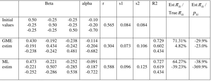
Table 1: Comparison of GME and ML estimates on a homothetic demand system with good starting values
Beta alpha r s1 s2 R2 Est
ki
π
/ Trueπ
ki Estπ
ki/ ki p Initial values 0.50 -0.25 -0.25 -0.25 0.50 -0.25 -0.25 -0.25 0.50 -0.10 -0.20 -0.70 0.565 0.084 0.084 GME estim 0.430 -0.191 -0.238 -0.192 0.434 -0.242 -0.238 -0.242 0.481 -0.114 -0.204 -0.682 0.304 0.073 0.106 0.729 0.602 0.434 71.31% 4.82% -29.9% -23.0% ML estim 0.473 -0.221 -0.252 -0.221 0.507 -0.286 -0.252 -0.285 0.538 -0.091 -0.187 -0.722 0.588 0.096 0.125 0.727 0.619 0.434 64.27% -39.23% -38.9% -369.9%Structural parameters estimated through ML seem to be a bit closer to true parameters than those estimated through GME. However virtual prices estimated by GME (notably good 2) are closer to “true” virtual prices than those estimated by ML. This probably explains why the qualities of adjustment for all equations are nearly the same for both methods.
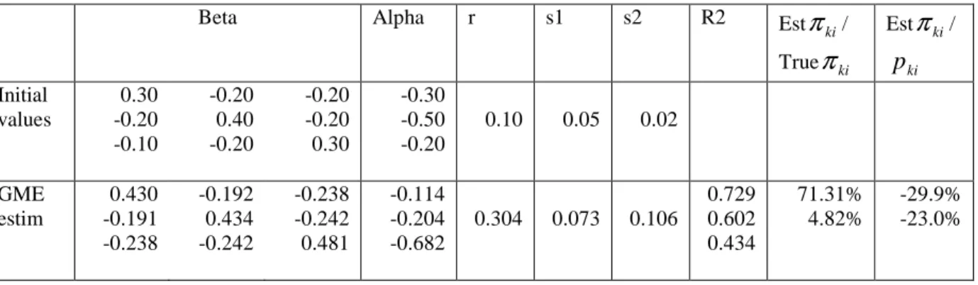
We secondly adopt different starting values: two interesting empirical results appear. Firstly the ML approach does not always lead to a solution while we always get one with the GME one. Secondly the econometric results obtained with the GME are rather independent of these initial values. This indicates a good stability of the method. For instance table 2 reports the
GME econometric results with new starting values while the ML program fails to converge. Our tentative interpretation of these results is the following. The concavity condition is explicitly introduced as a firm constraint in the GME program (see program 29) while only implicit in the derivation of the likelihood expression. Accordingly, when solving the GME program the optimisation procedure first searches for a feasible region of structural parameters and virtual prices, and then maximises the objective function. On the other hand, the ML program does both simultaneously and may have difficulties between the optimisation of the likelihood function and the satisfaction of theoretical conditions.
Table 2: GME estimation of a homothetic demand system with poor starting values
Beta Alpha r s1 s2 R2 Est
ki
π
/ Trueπ
ki Estπ
ki/ ki p Initial values 0.30 -0.20 -0.10 -0.20 0.40 -0.20 -0.20 -0.20 0.30 -0.30 -0.50 -0.20 0.10 0.05 0.02 GME estim 0.430 -0.191 -0.238 -0.192 0.434 -0.242 -0.238 -0.242 0.481 -0.114 -0.204 -0.682 0.304 0.073 0.106 0.729 0.602 0.434 71.31% 4.82% -29.9% -23.0%c. Econometric results on the non homothetic case
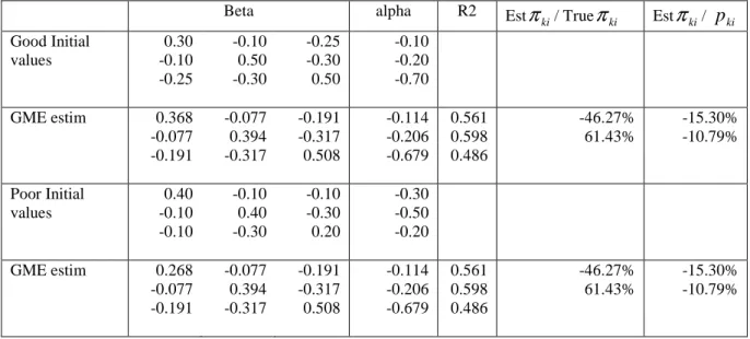
One great advantage offered by our solution is the possibility to estimate zero censored non homothetic demand system. Our estimation program in this case is more non linear than in the homothetic case. Accordingly we again test the sensitivity of the results to starting values. Results reported in table 3 show again a great stability of GME results with respect to these initial values.
Table 3: GME estimation of a non homothetic demand system with good and poor starting values
Beta alpha R2 Est
ki
π
/ Trueπ
ki Estπ
ki/ pki Good Initial values 0.30 -0.10 -0.25 -0.10 0.50 -0.30 -0.25 -0.30 0.50 -0.10 -0.20 -0.70 GME estim 0.368 -0.077 -0.191 -0.077 0.394 -0.317 -0.191 -0.317 0.508 -0.114 -0.206 -0.679 0.561 0.598 0.486 -46.27% 61.43% -15.30% -10.79% Poor Initial values 0.40 -0.10 -0.10 -0.10 0.40 -0.30 -0.10 -0.30 0.20 -0.30 -0.50 -0.20 GME estim 0.268 -0.077 -0.191 -0.077 0.394 -0.317 -0.191 -0.317 0.508 -0.114 -0.206 -0.679 0.561 0.598 0.486 -46.27% 61.43% -15.30% -10.79%d. Empirical properties of estimators
So far we only discuss the econometric results in terms of existence of solution, the quality of adjustment and the sensibility to starting values. We now focus on the precision of the estimates. As said earlier, delivering and/or computing the asymptotic properties of all estimators are challenging and we rely here on bootstrap inference techniques.
Basically the bootstrap is a re-sampling procedure which allows computing the MSE for each method. In a nutshell, the principle of this procedure is as follows in a simple case as equation (22). Let B be the number of bootstrap samples. We then apply B times the following two steps. First we draw randomly and with replacement from an initial sample (Y,X) a sample of the same dimension noted (Y*, X*). Second we estimate the model on this sample and get estimated parameters
β
*. Once this is done, we are able to compute the mean and variance ofβ
* on the B bootstrap samples as well as the MSE criterion. It is defined as the sum of the variance and the squared bias:(
)
2( )
* *
MSE =
β β
− +Varβ
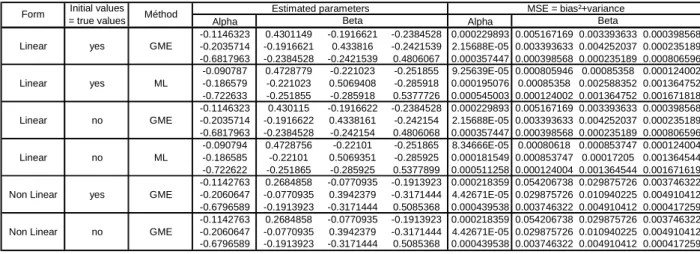
As expected, results reported in table 4 show that GME and ML econometric results converge on the homothetic case in terms of MSE. The MSE obtained with the non homothetic case are not directly comparable to homothetic ones but still we do not observe radical changes. This gives one first empirical support to our solution.
Table 4: Properties of GME and ML estimators: results from bootstrapping
7. Concluding comments
The econometric estimation of zero censored demand system faces major difficulties. The virtual price approach pioneered by Lee and Pitt (1986) in an econometric framework is theoretically consistent but empirically feasible only for homothetic demand system, and even may fail to converge depending on initial conditions. In this paper we propose to expand on this approach by relying on the generalized maximum entropy concept instead of the Maximum Likelihood paradigm. The former is robust to the error distribution while the latter must stick with a normality assumption. Accordingly the econometric specification of censored demand systems with virtual prices is made easier even with non preferences defined over several goods. Illustrative Monte Carlo sampling results show its relative performance.
There are several extensions to this paper that must be contemplated before getting definitive statements on this long standing issue. In the Monte Carlo experiments reported in this paper we only consider three good demand systems. We also try a five good demand system with the GME approach and we face no econometric difficulties. Nevertheless it will be interesting to test the method in more contrasting cases with larger shares of zero points for instance. The difficulty we had to deal with up to now is not to estimate but rather to simulate in the very first step a consistent dataset. In particular our experience shows that it is crucial to maintain the often overlooked condition that marginal utility of income must be positive. In that respect we fully agree with Barnett (2002) that complete respect of all theoretical conditions is very crucial.
Alpha Alpha
-0.1146323 0.4301149 -0.1916621 -0.2384528 0.000229893 0.005167169 0.003393633 0.000398568
Linear yes GME -0.2035714 -0.1916621 0.433816 -0.2421539 2.15688E-05 0.003393633 0.004252037 0.000235189
-0.6817963 -0.2384528 -0.2421539 0.4806067 0.000357447 0.000398568 0.000235189 0.000806596 -0.090787 0.4728779 -0.221023 -0.251855 9.25639E-05 0.000805946 0.00085358 0.000124002
Linear yes ML -0.186579 -0.221023 0.5069408 -0.285918 0.000195076 0.00085358 0.002588352 0.001364752
-0.722633 -0.251855 -0.285918 0.5377726 0.000545003 0.000124002 0.001364752 0.001671818 -0.1146323 0.430115 -0.1916622 -0.2384528 0.000229893 0.005167169 0.003393633 0.000398568
Linear no GME -0.2035714 -0.1916622 0.4338161 -0.242154 2.15688E-05 0.003393633 0.004252037 0.000235189
-0.6817963 -0.2384528 -0.242154 0.4806068 0.000357447 0.000398568 0.000235189 0.000806596 -0.090794 0.4728756 -0.22101 -0.251865 8.34666E-05 0.00080618 0.000853747 0.000124004
Linear no ML -0.186585 -0.22101 0.5069351 -0.285925 0.000181549 0.000853747 0.00017205 0.001364544
-0.722622 -0.251865 -0.285925 0.5377899 0.000511258 0.000124004 0.001364544 0.001671619 -0.1142763 0.2684858 -0.0770935 -0.1913923 0.000218359 0.054206738 0.029875726 0.003746322
Non Linear yes GME -0.2060647 -0.0770935 0.3942379 -0.3171444 4.42671E-05 0.029875726 0.010940225 0.004910412
-0.6796589 -0.1913923 -0.3171444 0.5085368 0.000439538 0.003746322 0.004910412 0.000417259 -0.1142763 0.2684858 -0.0770935 -0.1913923 0.000218359 0.054206738 0.029875726 0.003746322
Non Linear no GME -0.2060647 -0.0770935 0.3942379 -0.3171444 4.42671E-05 0.029875726 0.010940225 0.004910412
-0.6796589 -0.1913923 -0.3171444 0.5085368 0.000439538 0.003746322 0.004910412 0.000417259
Estimated parameters MSE = bias²+variance
Beta Beta
Form Initial values = true values Méthod
Another extension is to confront this approach to real datasets and contrast it to other methods. Real datasets are always more difficult to analyse than built-ones due to endogeneity and/or multi-collinearity issues for instance. According to results reported by van Akkeren et al. (2002) we are quite confident that our approach will allow managing these cases but this is to be checked.
Finally our approach allows estimating simultaneously and explicitly structural parameters and virtual prices. In the entropy objective function, one has the possibility to weigh one component relative to the others. For instance one may improve the prediction or the precision of the estimates depending on its own objective (Golan et al., 1996). It may be interesting in some cases to focus on the virtual prices and in other cases on the structural parameters. Additional works may explore deeper this possibility.
References
Arndt, C., Liu, S., Preckel, P.V. (1999). On dual approaches to demand systems estimation in the presence of binding quantity constraints. Applied Economics, 31: 999-1008.
Barnett, W.A. (2002). Tastes and technology: curvature is not sufficient for regularity. Journal of Econometrics, 108: 199-202.
Barnett, W., Pasupathy, M. (2003). Regularity of the generalized quadratic production model: a counterexample. Econometric Reviews, 22: 135-154.
Gallant, A.R., Gollub, G.H. (1984). Imposing curvature restrictions on flexible functional forms. Journal of Econometrics, 26: 295-322.
Golan, A., Judge, G.G., Miller, D. (1996). Maximum Entropy Econometrics: Robust Estimation With Limited Data. John Wiley & Sons.
Golan, A., Judge, G.G., Perloff, J. (1997). Estimation and inference with censored and ordered multinomial response data. Journal of Econometrics, 79: 23-51.
Golan, A., Perloff, J., Shen. E. (2001). Estimating a demand system with nonnegativity constraints: Mexican meat demand. The Review of Economics and Statistics, 83(3): 541-550.
Haveman, J., Hummels, D. (2004). Alternative hypotheses and the volume of trade: the gravity equation and the extent of specialization. Canadian Journal of Economic, 37: 199-218.
Hasan, M., Mittelhammer, R.C., Wahl, T.I. (2002). Simulated maximum likelihood estimation of a consumer demand system under binding non negativity constraints: an application to Chinese household food expenditure data. Working paper, Washington State University. Lau, L.J. (1978). Testing and Imposing Monotonicity, Convexity, and Quasi-Convexity
Constraints. In Production Economics: A Dual Approach to Theory and Applications (Vol.&), eds Fuss, M., McFadden, D. Amsterdam: North-Holland, 409-453.
Lee, L.F., Pitt, M.M. (1986). Microeconometric demand systems with binding nonnegativity constraints: the dual approach. Econometrica, 54: 1237-1242.
Moschini, G. (1999). Imposing local curvature conditions in flexible demand systems. Journal of Business & Economic Statistics, 4: 487-490.
Neary, J.P., Roberts, K.W.S. (1980). The theory of household behaviour under rationing. European Economic Review, 13: 25-42.
Newey, W.K., McFadden, D. (1994). Estimation and Hypothesis Testing in Large Samples. In Engle, R.F., McFadden, D. (eds.), Handbook of Econometrics, Vol. 4, Amsterdam: North-Holland.
Romer, P. (1994). New goods, old theory, and the welfare costs of trade restrictions. Journal of Development Economics, 43(1): 5-38.
van Akkerren, M., Judge, G., Mittelhammer, R. (2002). Generalized moment based estimation and inference. Journal of Econometrics, 107: 127-148.
van Soest, A., Kooreman, P. (1993). Coherency and regularity of demand systems with equality and inequality constraints. Journal of Econometrics, 57: 161-188.
van Soest, A., Kooreman, P. (1988). Coherency of the indirect translog demand system with binding nonnegativity constraints. Journal of Econometrics, 44: 391-400.
Wales, T. J., Woodland, A. D. (1983). Estimation of consumer demand systems with binding non-negativity constraints. Journal of Econometrics, 21: 263-285.
Yen, S.T., Lee, B.H. (2006). A sample selection approach to censored demand systems American Journal of Agricultural Economics, 88(3): 742-749.
Annex 1: Derivation of the likelihood function when only good one is not consumed
We have two possibilities to get this expression and explore both below.
Solution 1: l(w1i,w2i/xi)=P
(
e1i ≤−B1i/w2i,xi)
P(w2i/xi)This likelihood expression implies to know the law of w2i subject to data:
(
)
i i i i i i i i i i i i i R p e B R e R R p B w 1 1 1 11 1 1 1 11 1 11 1 1 ln 1 ln 0 ln ln 0 + − − = ⇔ = + + − ⇔ = β π π β βSo, when replacing
i i R 1 lnπ in w2i expression, we get:
(
)
(
i i)
i i i i i i i i i i i i e e B B w e R p e B R p B w 2 1 1 11 21 2 2 2 1 1 1 11 21 1 21 2 2 ln 1 ln − + + − = ⇔ − + − − − + − = β β β β β Let: 11 21 1 1 11 21 2 0β
β
α
β
β
α
i =−Bi + Bi and i = which gives: w2i =α0i+α1ie1i−e2iAs a linear combination of normal distributions, w2i follows a normal law:
i i i i i i E e E e w E( 2 )=
α
0 +α
1 ( 1 )− ( 2 )=α
0 and V(w2i)=α²1iV(e1i)+V(e2i)−2α1icov(e1i,e2i)=α12is12+s22−2α1irs1s2) 2 , ( 0 12 12 22 1 1 2 2 N s s rss wi ≈ αi αi + − αi − + − − + = − + = 1 , 0 ; 2 2 1 ) 2 , ; ( ) / ( 2 1 1 2 2 2 1 2 1 0 2 2 1 1 2 2 2 1 2 1 2 1 1 2 2 2 1 2 1 0 2 2 s rs s s w f s rs s s s rs s s w f x w P i i i i i i i i i i i i
α
α
α
α
α
α
α
α
Moreover, i i i i i e w e 1 2 0 2 1 α α + −= , thus e1i/w2i is a linear function of e2i: this random variable follows a normal law.
) / (e1i w2i
E is the orthogonal projection of e1i on the space generated by w2i: