Detection and Estimation Theory

Academic and Research Staff Prof. H. L. Van Trees Prof. D. L. Snyder Dr. A. B. Baggeroer

Graduate Students

M. F. Cahn T. J. Cruise M. Mohajeri

L. D. Collins A. E. Eckberg, Jr. E. C. Wert R. R. Kurth

A. THESES COMPLETED

1. STATE VARIABLES, THE FREDHOLM THEORY AND OPTIMAL COMMUNICATIONS

This study has been completed by A. B. Baggeroer. It was submitted as a thesis in partial fulfillment of the requirements for the Degree of Doctor of Science, Depart-ment of Electrical Engineering, M. I. T. , January 1968.

H. L. Van Trees

2. ASYMPTOTIC APPROXIMATIONS TO THE ERROR PROBABILITY FOR DETECTING GAUSSIAN SIGNALS

This study has been completed by L. D. Collins. It was submitted as a thesis in partial fulfillment of the requirements for the Degree of Doctor of Science, Department of Electrical Engineering, M. I. T. , June 1968.

H. L. Van Trees

3. CLOSED-FORM ERROR EXPRESSIONS IN LINEAR FILTERING

This study has been completed by M. Mohajeri. It was submitted as a thesis in partial fulfillment of the requirements for the Degree of Master of Science, Department of Electrical Engineering, M. I. T. , June 1968.

H. L. Van Trees

B. PERFORMANCE OF THE OPTIMAL SMOOTHER

The purpose of this report is to correct some errors in the analysis of the perfor-mance of the optimal smoother, which have appeared in recent publications.1,2

This work was supported by the Joint Services Electronics Programs (U. S. Army, U. S. Navy, and U. S. Air Force) under Contract DA 28-043-AMC-02536(E).

Let us assume that the generation of a state vector x(t) and its observation in the

presence of noise may be described by the following linear state representation and

covariance matrices:

dx(t)

dt

=

F(t) x(t) + G(t) u(t),

T

_o0

t;

(1)

r(t)

=

C(t) x(t)

+

w(t),

T

0

< t

< Tf;

(2)

E[u(t)_uT ()] = Q6(t-T), T

0<

t,T; (3)

Ex(T

)xT (T)] =

(To

T);

(4)

E[w(t)w (r)] = R(t) 6(t-T), T

0

t, T. (5)

(Zero means for u(t), x(To), and w(t) have been assumed for simplicity.)

The optimal smoother estimates the state vector x(t) over the interval

[To,

Tf], where

the received signal r(t) is observed over the same interval.

The equations specifying

the structure of the smoother may be found by assuming Gaussian statistics and using

variational means,1,2 or by using a structured approach and solving the resulting

Wiener-Hopf equation.3 This structure is

d

(t)

F(t)

G(t) QG (t)

x(t)

0

T

p(t)(t)

C (t) R

(t) C(t)

-F

(t)

(t)

(t)

(t)

r(t

(6)

with the boundary conditions

_(T)=

0

(T

IT

o

)

(To)

(7)

P(Tf) = 0.

(8)

One can also relate the optimal smoother estimate x(t) to the realizable filter estimate

A

2,3

Sr(t) by

g(t)

-

x

(t) =

(t

It)

p(t)

T

_°

t

<

T ,

(9)

-r

where Z (t

It)

is the realizable filter covariance of error.

Let us now consider some aspects of the performance of the smoother. First, we

have the result

T

that is, the smoother error E(t) = x(t) -x(t) is uncorrelated with the costate p(t) for all time within the observation interval.

Proof: The costate function p(t) is the result of a linear operation upon the received signal r(t). The error E(t) is uncorrelated with the received signal by the orthogonal projection lemma; see, for example, Van Trees4 or Kalman and Bucy.5 Equation 10 follows from this lemma and the linearity of the operation for finding the costate.

Our next result relates the smoother error covariance Z (t ITf), the realizable filter covariance Z (t t), and the costate covariance II(t ITf) by the formula

Z (t Tf) + (tt ) II(t IT) e (t t) = Z (t t), To < t Tf'1) Proof: Let us rewrite Eq. 9 in the form

E(t) -E (t) = 7 (t t) p(t), T < t < Tf, (12)

where we have subtracted and added x(t) to the left side of Eq. 9, and E (t) is the

realiz--r

able filter error. We can in turn rewrite Eq. 12 in the form

E(t) - (tt ) p(t) = Er(t), T < t < Tf. (13)

Equation 11 follows by multiplying (13) by its transpose, taking the expectation of the result, and using (10) to eliminate the cross-product terms between E(t) and p(t).

Our third result states that the covariance of the costate satisfies the matrix dif-ferential equation

d (t Tf) =-(F(t) - (tt) CT(t) R(t) C(Ct))T II(t Tf)

-I(t IT ) (F(t) -Z(tt

)

C (t) R-(t) C(t))

-C T (t) R-l (t) C(t), T _o t

<

T (14)

with the boundary condition II(Tf Tf) = 0, since p(Tf) vanishes identically.

Proof: We simply differentiate Eq. 11 with respect to the variable t and substitute the differential equations for 2 (t Tf) and Z (t It). The differential equation for Z (t T f) can be found by several methods to be2,3

d T(tf) = (F(t)+G(t) QGT(t) -1 (t t)) (t Tf) dt f

2

(t I Tf ) (F(t)+ G(t) QG T(t) Z-l1 (tt)) T -G(t) QG (t), To

4

t

<

Tf (15) -- Git

i15

with the final boundary condition 2 (Tf I Tf) provided by the realizable filter solution at t = Tf. The differential equation for Z (t It) is well known5

dt Z (t t) = F(t) Z (t t) + Z (t It) F T(t) + G(t) QGT (t)

T

o

< t,

₍₁₆₎

with the initial condition given by Z (To To). Making these substitutions and using the

positive definitness of Z (t It) yields the desired result.

One can determine a second set of differential equations for the smoother covariance

Z (tITf). Let us define two (2nX2n) matrices

P(t I Tf) P(t Tf) =

1f

(t ITf) F(t)

W(t)

= R- (t)C(t)

C (t)

R

1

(t) C(t)

-(t)(t T) (t _{f )} -I(t IT_f)

G(t) QG (t)

-FT (t)

By using Eqs. 11, 14, 15, and 16, it is a straightforward exercise to satisfies the following matrix differential equation

G(t) QG (t)

d P(t

I Tf)

=

W(t) P(t

IT

) + P(t

ITf)

WT(t)

+

0

show that P(t ITf)

0

CT ( t ) R-l ( t ) C(t) To _{t < Tf} 0 f P(Tf ITf) = (Tf Tf) 0 0 -0

Let us contrast these results with some that have been published.

Equa-tion 18a is identical in form to those given by Bryson and Frazier.1

Our

inter-pretation of the partitions of the matrix P(tITf), however, is quite different. We

have demonstrated that P(tITf) is not the covariance matrix of the augmented

vector of E(t) and p(t); that is,

P(t ITf) E -E(t)

_{E(t) T}

p M) p(t)

QPR No. 90

and T _{o t < Tf, (17a)} T 0< t < Tf. (17b) (18a) (18b)

(19)

-Z(t It) CT ( t ) R-l ( t ) C(t) (t It), 190

If this is true, we can easily demonstrate a contradiction by using Eq. 18:

dt n(t T)tf = T (Tf) R-1(T f) C(T f). (20)

-f

This in turn implies

II(T f-At

Tf)

= -CT(T f) R-1(Tf) C(Tf) C(Tf) At, (21)

which is clearly impossible, since II(t ITf) is a covariance matrix. We have also shown in Eq. 10 that the diagonal terms in the expectation indicated in Eq. 19 are zero.

In Rauch, Tung, and Striebel's paper on this topic, they also assert that the smoothing error E(t) and the costate p(t) are correlated. As indicated above, they are not. Also, their relation between Z (t ITf) and l(t ITf) differs from Eq. 11 with respect to sign,

which will imply the same negative covariance as discussed above.

While the basic result concerning the equation for 2; (t ITf) is correct in both of these papers, these differences and contradictions leave some of the derivation involved rather su spe ct.

A. B. Baggeroer References

1. A. E. Bryson and M. Frazier, "Smoothing for Linear and Nonlinear Dynamic Sys-tems," Proc. Optimum Synthesis Conference, Wright-Patterson Air Force Base, September 1962.

2. H. Rauch, F. Tung, and C. Striebel, "Maximum Likelihood Estimates of Linear Dynamic Systems," AIAA J. , Vol. 3, No. 8, August 1966.

3. A. B. Baggeroer, "State Variables, the Fredholm Theory, and Optimal Communica-tions," Sc. D. Thesis, Department of Electrical Engineering, Massachusetts Institute of Technology, January 1968.

4. H. L. Van Trees, Detection Estimation, and Modulation Theory, Part I (John Wiley and Sons, Inc., New York, 1968).

5. R. E. Kalman and R. Bucy, "New Results in Linear Filtering and Prediction Theory," ASMW J. Basic Eng., Vol. 83, pp. 95-108, March 1961.

C. ASYMPTOTIC APPROXIMATIONS TO THE ERROR PROBABILITY FOR SQUARE-LAW DETECTION OF GAUSSIAN SIGNALS

In Quarterly Progress Report No. 85 (pages 253-265) and No. 88 (pages 263-276), we discussed the application of tilted probability distributions to the problem of

evalu-ating the performance of optimum detectors for Gaussian signals received in additive Gaussian noise. In many situations it is convenient for either mathematical or physical reasons to use a suboptimum receiver. For example, instead of building a time-variant

linear estimator followed by a correlator, we may choose to use a time-invariant filter

followed by an envelope detector. In this report we develop the necessary modifications

to allow us to approximate the error probabilities for such suboptimum receivers. We

first derive an asymptotic expansion for the error probabilities. Since the test statistic

is not the logarithm of the likelihood ratio, we must calculate the semi-invariant

moment-generating function separately for each hypothesis. Second, we calculate these functions

for the class of suboptimum receivers consisting of a linear filter followed by a squarer

and an integrator. This is an accurate model for many of the receivers that are used

in practice. We shall concentrate on the case in which the random processes and the

receiver filter can be modeled via state variables. This includes as a subclass all

sta-tionary processes with rational spectra and all lumped RLC filters. In Section XVIII-E

some numerical results will be presented which were obtained by using the techniques

that we shall develop here.

The problem that we are considering is the zero-mean binary Gaussian problem.

H

1

: r(t) =

sl(t)

+ w(t)

T1• <t < Tf. ₍₁₎

HO:

r(t) = s

0

(t) + w(t)

s

l

(t) and s

0

(t) are sample functions from zero-mean Gaussian random processes with

known covariance functions Kl(t, T) and K (t, T), _{and w(t) is a sample function of white}

Gaussian noise with spectral density

N

0

/Z.

1. Approximations to the Error Probabilities

In this section, we develop bounds on and approximations to the error probabilities

for suboptimum receivers. The development for hypothesis

H

0

parallels that for the

optimum detector which was given in the previous report. We add a subscript to the

semi-invariant moment-generating function to denote the hypothesis

o0(s) = in MIH 0 (s)

=

in

E

eSI

Ho],

₍₂₎

where f denotes the test statistic on which the decision is based. For our purposes it

will suffice to consider s real. Furthermore, Eq. 2 is valid only over some range of s,

say a

<

s

<

_{b, which is the familiar "region of convergence", associated with a Laplace}

transform.

Now we define a tilted random variable

0s

to have the probability density

sL-

0

(s)

Then

Pr [E IH0

]

= p

Y

(L) exp[l

0

(s)-sL] dL,

f0s

where y denotes the threshold level. Just as before, we expand p

(L) in an Edgeworth

fOs

expansion. Therefore, we shall need the semi-invariants of the tilted random variable 10s, which are the coefficients in the power series expansion of the semi-invariant moment-generating function for i0s'

in

M s (t) =

in

E [et 0 s

Os

00 (s+t) L- (s) Sin e _pl

_{H (L) dL}

= 10(s+t) -

[0(s).

Therefore dk th d k (s) = k _{semi-invariant of 20s'} dsk s'

and the coefficients in the Edgeworth expansion of p

Os(L) are obtained from the deriva-0s

tives of p

0

(s) just as before.

Now we proceed with an analogous development for hypothesis

H

₁

.

tl (s) n MIHIHI(s).

For the optimum detector discussed previously, f =

in

A(r(t)),

where A(r(t)) is the likelihood ratio, and 1l(S) = 10(S+1),

so that it was sufficient for that case to consider only one of the two conditional moment-generating functions.

Returning to the suboptimum receiver, we must define a second tilted random vari-able i1s'

pls

(L) = e

PI H1

( s )

.

sL-[l(s)

Then, Pr [E1 _{1 = E}

p

2

s(L) dL.

is

Just as above

in

M (t) = L1(t+s) - tl(S), Is and

dk

ds

ds

I ( s ) = kt h _{semi-invariant of} 2_i1s'

so that the coefficients in the Edgeworth expansion of p 1s(L) are obtained from the derivatives of 4l( ) .

Our bounds and approximations follow immediately from Eq. 4 and 7.

bounds are

Pr [E IH]

<

exp[4

0

(s

0

)-s

0

y]

Pr [

IH1]

<

exp[pl(s)-sly]

The Chernoff

for s

o

> 0

for s

₁

<0,

(10)

(11)

where

(12)

and

IL

1( 1) =

Y.

Similarly, the first-order asymptotic approximations are 2

S[)

₊

Pr

[IHO] z(-s04D

)

exp 0(s0 -s 0(s

o

+

0s0

(13) (14) 2 s exp l(sl) I spl(s1) + l(sl , Pr [E H1] (15)

where so and s1 are given by Eqs. 12 and 13, and #(X) is the Gaussian error function

4(X) =

i--

exp [2 dx. (16)

Since

o(So) =

=(s)

= Var (J0s)

0

(17)

1 (S) = Var (fIs) 0,

0 (s) and l(s) are monotone increasing functions of s.

Then Eq. 12 has a unique solu-tion for s0 > 0 if

y 0(0) = E[f H0

].

(19)

Equation 13 has a unique solution for s -< 0 if

y

(0)

=

E[f H

1

].

(20)

Thus, just as for the optimum receiver, we require

E[ JH0] < y < E[f H1] (21)

in order to be able to solve Eqs. 12 and 13. This restriction is in addition to that implied in the definition of the function 0 (s) and

p

1(s).

We have developed bounds on and approximations to the error probabilities for a rather general binary detection problem. The semi-invariant moment-generating func-tions

4j(s)

played a central role in all of our results. These results were obtained

with-out making any assumptions on the conditional statistics of the received signals. We shall now evaluate Lj(s) for a specific class of Gaussian random processes and subopti-mum receivers.

2. Semi-Invariant Moment-Generating Functions for Square-Law Detectors

The class of suboptimum receivers that we shall consider is indicated in Fig. XVIII-1. For the class of problems that we are considering, r(t) and y(t) are Gaussian random processes. Expanding y(t) in its Karhunen-Lobve expansion

00 t) yi(t) Ti t < Tf, (22)

i=l

we have S=f

y

2(t) dt 90 00 = Yi .(23)

i=l

Hence, I is the sum of squares of statistically independent Gaussian random variables

and all of our previous discussion about the inapplicability of the Central Limit

The-orem to p (L) still holds.

It is still natural, however, to proceed from a

charac-teristic function or moment-generating function point of view.

(s)

=

fn E esf

Hj1

= n

E

exp s

Y

jH

i=l

=

n E exp (sy2)

H

i=l

00

Sin

(1

-2sX)

for s <

,

j

=

0, 1,

(24)

i= 1

13i

where {Xij

}

denotes the eigenvalues of y(t), T

i

- t < T,

conditioned on H., for j = 0, 1;

and we have used Eq. 7.67 of Wozencraft and Jacobs.

2

r(t)

y(t)

Y (t)

T

--

h (t, r)

SQdt

T.

Fig. XVIII-1.

A class of suboptimum receivers.

The problem of computing the output probability distribution of a nonlinear detector,

such as that shown in Fig. XVIII-1, has been studied for more than twenty years.

3

_The

previous approaches to this problem started with an expression for the characteristic

function analogous to Eq. 24.

Only recently has a satisfactory technique for finding the

significant eigenvalues become available.4 We thus can approximate the characteristic

function by using the most significant eigenvalues.

We are then faced, however, with

the computational problem of evaluating (numerically) an inverse Fourier transform.

Although highly efficient algorithms exist,5 the constraint of computer memory size

makes it difficult to obtain sufficient accuracy on the tail of the probability density.

Instead, we use the moment-generating function (with real values for its argument)

to obtain bounds and approximations as discussed above. All that remains is to obtain

closed-form expressions for 0j(s) and l(s). Recall that the Fredholm determinant for a random process y(t), T.i t < Tf, is defined as

o00

D (z) (l+zki), i=l

where

({Xi}

are the eigenvalues of y(t).

Then from Eq. 23,

1

j (s) -

In

DS H (-2s)

(25)

1

for s <

I7-j, j

=

0, 1.

(26)

The restriction on s below Eq. 26 is the "region of convergence" discussed above.

Combining this with the ranges on s for which Eqs. 12 and 13 have a solution, we have

0

< < 0 _2Xi 0

and

S1 i < 0. (27a) (27b)

The techniques discussed in the previous report for evaluating Fredholm deter-minants are applicable here, too. Here the pertinent random process is the input to the square-law device in the receiver, conditioned on the two hypotheses. In the case in which the random-process generation and the receiver filter can be modeled via state variables, we can readily evaluate the Fredholm determinant. The model, conditioned

w(t)

Fig. XVIII-2. Suboptimum receiver: State-variable model.

on one of the hypotheses, is shown in Fig. XVIII-2. For simplicity in the discussion that follows, we drop the subscript denoting the hypothesis.

The equations specifying the message generation are

2

1

(t) = F (t) x(t)

+

Gl(t)

ul(t)

r(t)

=

C (t) x (t) + w(t),

(28a)

(28b)

S1 (t)

and those specifying the receiver are

2

(t) = F

2

(t) x (t) + G

2

(t) r(t)

y(t) =

C

2(t) x2(t).

The initial conditions are zero-mean Gaussian random variables.

E

l (Ti) xT(T

P

E x₂

(T)

(Ti)

_I

_0.

The entire system can be rewritten in canonical state-variable form.

d x1 (t)

F (t)

dtd

x2L(t)i

L

_(t)C

₁

r

1

(T.)

1

T

T

E

fxi

(T),XZ(T

LLx2(T)j

Define

0

x

(t)

M

G (t)

F (t) x (t)

0

P 0

-0 --0 0

0 7 u I(t)

G

2

(t) W(t)

__

(t(t)

2(t)t) =l(t)

G (t)

=(t)

0 G 2(t)

Qt)

=

0

0

N

(t -T N

2

C(t) =

[o,_C

2(t)] (29a) (29b) (30a) (30b)

(31a)

(31b)

(32a)

(32b)

(32c)

(32d) (32e)

u

1

(t)

u(t) =

Lw(t)

J

10

0

0

0

x(t)

=

F(t) x(t) + G(t) u(t)

y(t)

=

C(t) x(t)

E[(t) x (t)] = _ _{o ,}

and the evaluation of the Fredholm determinants is carried out exactly as before,6 using

in D (z) =

in

det _2(Tf) +

(t)

F (t)

d

dt 2(t T(t) zC(t) - 2 i(T d

f Tr [F(t)] dt,

ST.

T

F

-t

T

2

G

-

(t)

t)

L(t

(t)i

-F

(t)

~

~2(t)

3. Application to Stationary Bandpass Random Processes

In many applications, the random processes of interest are narrow-band around some carrier frequency

o

. That is,

s(t) = NIT A(t) cos (wct+0(t)),

(36)

where the envelope and phase waveforms, A(t) and 0(t), have negligible energy at

fre-quencies comparable to oc. Equivalently, we can write s(t) in terms of its quadrature

components.

s(t)

= Ns

So(t) cos

oct +

NITs

(t)

sin

c

t.

(37) Then

(32f)

(32g)

(33a) (33b) (33c) where (34) (35a) (35b)

In some of our applications we shall consider stationary bandpass random processes that can be modeled as in Eq. 37 over some interval T. < t < Tf, where s (t) and s (t) are statistically independent stationary random processes with identical statistics. For this case, the eigenvalues of the bandpass random process s(t) are equal to the

eigen-values of the quadrature components. Each eigenvalue of s c(t) and ss(t) of multiplicity N is an eigenvalue of s(t) with multiplicity 2N. It follows immediately that

BP N-= 2 LP

(

N-) (38)

where the subscripts BP and LP denote "bandpass" and "lowpass," and we have explicitly indicated the signal-to-noise ratio in each term.

We comment that the results in Eq. 38 are not the most general that can be obtained for bandpass processes, but they suffice for the examples that we shall consider. A more detailed discussion of properties and representation for bandpass signals would take us too far afield. There are two appropriate references.7, 8

4. Summary

In this report we have discussed the necessary modifications of our asymptotic approximations to error probabilities to allow us to analyze suboptimum receivers. The results were expressed in terms of two semi-invariant moment-generating functions. For the problem of square-law detection of Gaussian signals, these functions can be expressed in terms of the Fredholm determinant. For the important case of processes and systems that can be modeled via state variables, there is a straightforward technique available for computing their Fredholm determinants.

In Section XVIII-E numerical results obtained by using the techniques developed in this report will be presented. A second problem in which these results have been suc-cessfully applied is the random phase detection problem.9 For this problem the received signals are not Gaussian, but since we can compute j(s), the approximations presented here are still useful.

L. D. Collins, R. R. Kurth

References

1. W. B. Davenport and W. L. Root, An Introduction to the Theory of Random Signals and Noise (McGraw-Hill Book Company, New York, 1958), Chap. 6.

2. J. M. Wozencraft and I. M. Jacobs, Principles of Communication Engineering (John Wiley and Sons, Inc., New York, 1965), p. 522.

3. Davenport and Root, op. cit., Chap. 9.

4. A. B. Baggeroer, "A State-Variable Technique for Solving Fredholm Integral Equa-tions," Technical Report 459, Research Laboratory of Electronics, M. I. T. , Cam-bridge, Mass., November 15, 1967.

5. J. Cooley and J. Tukey, "An Algorithm for the Machine Calculation of Complex Fourier Series," Mathematics of Computation, Vol. 19, April 1965.

6. L. D. Collins, "Closed-form Expressions for the Fredholm Determinant for State-variable Covariance Function," Proc. IEEE 56, 350-351 (1968).

7. H. L. Van Trees, Detection, Estimation, and Modulation Theory, Part II (John Wiley and Sons, Inc., New York, in press), Chap. 4.

8. A. Baggeroer, L. D. Collins, and H. L. Van Trees, "Complex State-Variables, The-ory and Applications," a paper to be presented at WESCON, Los Angeles, California, August 20, 1968.

9. L. D. Collins, "Asymptotic Approximations to the Error Probability for Detecting Gaussian Signals," Sc. D. Thesis, Department of Electrical Engineering, Massa-chusetts Institute of Technology, May 20, 1968.

D. CHANNEL CAPACITY FOR AN RMS BANDWIDTH CONSTRAINT

The usual definition of the channel capacity of a bandlimited additive noise channel implies that the channel is strictly bandlimited. In some applications a strictly band-limited assumption cannot be realistically imposed on the transmitted signal and/or channel. For example, a transmitted signal of finite duration is obviously not strictly bandlimited. Comparison of the performance of such an approximately bandlimited sys-tem with the theoretical performance implied by the strictly bandlimited channel capac-ity can lead to contradictions (such as system performance better than the "theoretical" ultimate performance). In this report the strictly bandlimited assumption of channel capacity is replaced by a mean-square bandwidth (rms) constraint and the resulting chan-nel capacity is computed.

1. Derivation of rms Bandlimited Channel Capacity

As is well known, the channel capacity of an additive white noise channel (spectral density No/2) for which the transmitter spectrum is S(f) is

C =iSo

df

in ₁

+2S(f)

(1)

It is convenient to define a normalized spectrum, o(f)

S(f) = Pr(f), (2)

where P is the average transmitted power which is assumed finite. Equation 1 becomes

C

42

df in

(~+

(f)) nats/sec. (3)

or channel constraints. Here an infinite bandwidth channel is assumed with power and bandwidth constraints on the transmitter.

For example, if a strictly bandlimited constraint is made at the transmitter

a-(f) = 0 If >W (4)

and the optimal choice of a-(f) is

cr(f)

=

2

If < W

with the resulting well-known capacity formula from Eq. 3:

C = W n (1 +

P

.

N W

_O

Defining a signal-to-noise ratio X in the transmitter bandwidth

N W

implies that the channel capacity increases logarithmically with increasing

signal-to-noise ratio.

For an rms bandwidth B constraint at the transmitter,

2

=

o

B

dff

20-(f),

which represents a constraint on cr(f). The other implied constraints are

a-(f) > 0

df o-(f) = 1.

₍₁₀₎

-oo

In order to maximize Eq. 3 subject to the three constraints on o-(f) (Eqs. 8-10), define

df fn

1 2P

0-(f)

+

a

c-O

-00oo

where a and y are Lagrange multipliers.

Perturbation of J with respect to -c(f)

yields

(11)

00

J =ioo

(f) = max N

La

2 a+yf

(12)

The maximum operation is necessary to satisfy o-(f) > 0. Clearly, if a, y are positive, a(f) = 0, which does not satisfy the constraint Eqs. 8 and 10. Similarly, if the two mul-tipliers are of different sign, the constraints cannot be satisfied; hence, a and y are both negative. Define two new positive multipliers •

Q

and fc such thatC

o(f)

= max 0, 1

2BX

(13)

where the signal-to-noise ratio in the rms bandwidth P

N B (14)

has been introduced. The transmitter spectrum is that of a one-pole process shifted

-- Q LARGE Q0 SMALL

Fig. XVIII-3.

down to cutoff

small

Q.

For -(f) as

Optimum transmitted spectrum for rms bandlimited channel.

at f

=

fc; the spectrum shape is plotted in Fig. XVIII-3 for large and

given in Eq. 13, direct evaluation of the constraints Eqs. 8 and 10 yields

XB3 = f

3

-+ -

+

tan-

Q

and

B = fc

Q+ Q

tan-

Q-1

.

(16)

These two equations determine the unknowns f and Q. Given f and Q as the solution of these equations, the channel capacity from Eq. 3 is

C = 2f

c

l-

tan

Q

.

It can be shown from the equations above that C can also be written

C

=

Bg(X),

(17)

(18) where g(X) is a complicated implicit function. The important observation is that channel capacity for rms bandwidth is of the same functional form as the strictly bandlimited form (Eq. 6), providing signal-to-noise ratios in the transmitter bandwidth are defined. Unfortunately g(k) is implicit and cannot be determined analytically.

(12 X)l

in (+ X)

10 100

Fig. XVIII-4.

Channel capacity per unit rms bandwidth.

tu

2. Large Signal-to-Noise Ratio Approximations

The equations can be solved approximately for X >> 1. For large Q the channel capac-ity in Eq. 17 is

C = 2f .

_c

(19)

Similarly, for large Q, Eq. 15 implies 2 f3 kXB3

(20)

-S c

or combining

C

=

B(12)1/3 X

1 / 3

(X>>1)

(21)

which implies that channel capacity increases as the cube root of X for an rms con-straint, but only logarithmically for a strict bandwidth constraint. Thus, using the strict bandwidth capacity formula for channels that are actually rms bandlimited yields a capacity much lower than the true capacity.

g(X) is plotted in Fig. XVIII-4 along with its asymptote (Eq. 21).

T. J. Cruise

E. PERFORMANCE OF A CLASS OF RECEIVERS FOR DOPPLER-SPREAD CHANNELS

This report considers a class of generally suboptimum receivers for the binary detection of signals transmitted over a Doppler-spread channel and received in additive white Gaussian noise. Bounds on the error probabilities for these receivers are given. The performance of a suboptimum system is compared with the optimum one in several example s.

In the binary detection problem one of two narrow-band signals

f.(t) = N Re

Lf(t)

e c , 0 < t < T, i = 0, 1, (1)

is transmitted over a Doppler-spread channel and received in additive white Gaussian noise. The complex envelope of the received signal is

r(t) b.f.(t) + w(t) 11

where bi(t) and w(t) are zero-mean, independent, stationary, complex Gaussian pro-cesses. Details of the representation of complex random processes may be found in Van Trees.1

The binary detection problem thus becomes one of deciding between the two hypoth-eses

H: r(t) = s1(t) + w(t)

0o

t < T. (3)

Ho:

r (t) = so(t) + w (t)

The known complex covariance functions for s.(t) and w(t) are K- (t, u) and N 6(t-u).

1 S. O

From Eq. 2, 1

K- (t,u) = fi(t) K .(t-u) fi (u), i = 0, 1. (4)

si

₁

i

b

₁

-(The superscript star denotes complex conjugation.)

A special case of this hypothesis test occurs when the f.(t) have identical complex 1

envelopes but carrier frequencies that are separated enough so that the f.(t) are orthog-1 onal. Then

H1: r(t) = N

Re ['(t) e

j

+ w(ty

H : r(t) = N Re (t) e + w(t), (5a) O where s(t) = b(t) f(t). (5b)

This model will be called the binary symmetric orthogonal communication case. 1. Optimum Receiver and Its Performance

The optimum receiver for the detection problem of Eq. 3 for a large class of criteria is well known1: the detector compares the likelihood ratio to a threshold. An equivalent test is

T

T

H

1

r (t) r(u) [h(t,u)-h o(t, u)] dtdu

<

y.

(6)

o Y0

H

The hi(t,u) are the complex envelopes of the bandpass filter impulse responses that satisfy the integral equations

N h.(t, u) +

K-(t,

x) h.(x,u) dx = K (t, u), 0

<

t,u

<

T, i = 0, 1. (7)

01 S. 1 S

0

1 1

For the binary symmetric orthogonal communication case with equally likely hypotheses, the threshold y is zero and the test of Eq. 6 reduces to choosing the larger of

. T

T

S

=

_i

r. (t) h(t, u) r.(u) dtdu,

i = 0, 1.

(8)

The subscript i indicates that the lowpass operation on the right-hand side of Eq. 8 is performed twice, once with rl(t) obtained by heterodyning r(t) from cl, and the other

1 , 1

with _o (t), the result of heterodyning r(t) from w . The filter h(t,u) satisfies Eq. 7 with

O O

the kernel K-(t, u) of the signal in Eq. 5b.

s 1-3

Bounds on the performance of the optimum receiver are known. For the detector of Eq. 6

P(E Ho)

<

exp[L(s)-sy]

0z<s

1

(9)

P(EjH1)

<

exp[p(s)+(1-s)y]

where

L N)0N

h(s)

=

sln 1+-

+ (1-s)1n

1+-j)-ln 1+

N

(10)

The

kil

and

kio

are the eigenvalues of the complex random processes s1(t), s0(t) of Eq. 2, respectively, under H .

_o

The . op are the eigenvalues of the composite

pro-1

comp

cess with covariance function

K (t, x) = (l-s) K- (t,x) + sK, (t, x). (10a)

comp

s1

s

The value of s is chosen to minimize the bounds in Eq. 9. In the binary communication problem the processes sl(t) and so(t) have essentially orthogonal eigenfunctions, and the probability of error for the detector of Eq. 8 is bounded4 by

exp

pc())

_{exp (c())}

< P(E) 1+ (11)

2 (I +

i!'c(+)

2(1

i

(s)

n

1

+ 1-

ln

(+

(In

N

1-

O

s

<

1.

(12)

The subscript c in Eqs. 11 and 12 denotes the binary symmetric orthogonal

communica-tion problem.

_{The Xi are the eigenvalues of the process '(t) in Eq. 5b. The functions}

L

c(s) and L(s) can be expressed as integrals of minimum mean-square filtering errors

and can be evaluated easily when the random processes '.(t) have state-variable

repre-sentations.

_{Collins presents details on this and on other approximations to the error}

probabilitie s.

If the eigenvalues in Eq. 12 are chosen to minimize [Lc(s), subject to a constraint on

the average received energy Er, a bound on the probability of error for a binary

orthog-onal communication system results3

P(E) -

exp -0.

1 4 8 8 .

₍₁₃₎

Thus Eq. 13 gives a bound on the exponential performance of any signal and receiver

for the communication problem of Eq. 5.

2.

Suboptimum Receiver

One implementation of the optimum receiver follows directly from Eq. 6 if the filter

i.(t, u) is factored

1

hi(t, u) =

gi(x, t) gi (x, u) dx,

O < t, u < T.

(14)

Then the optimum receiver is realized as the filter-squarer configuration of

Fig. XVIII-5.

_{At bandpass these operations correspond to a narrow-band filter followed}

by a square-law envelope detector and integrator.

Solving Eqs. 7 and 14 for 'i(t, u) is difficult in general, but for several special cases

the solution is possible and motivates the choice of the suboptimum receiver. The first

case occurs when the observation interval T is large and the process s'.(t) is stationary.

This implies that f(t) is a constant and the filter gi(t, u) is time-invariant.

Its Fourier

transform is

Gi(0) = ₍₁₅₎

s

~i~

+ N

v.(t)= vi(t)12

Fig. XVIII-5. Filter-squarer receiver for the binary detection problem.

'i(t) "bi(t)

FADING PROCESS CHANNEL I RECEIVER BRANCH

Fig. XVIII-6.

r(t)

XV---7.

Fig. XVIII-7.

State variable model for a Doppler-spread channel and the ith branch of the filter-squarer receiver.

W

(t)

F -r

Suboptimum receiver branch with signal multiplica-tion and time-invariant filtering.

(realizable gi(t)).

S- (w) is the Fourier transform of K~ (t-u).

_S.

S.

1 1

Another case in which the filter gi(t, _{u) can be found is under a low-energy coherence,} or "threshold" assumption. _{In this situation the impulse response h.(t,u) becomes}

1

K- (t,u). _{From Eqs. 4 and 14, this implies that for a large observation interval T the} 1

filter gi(t,u) is cascade of a time-variant gain, f (t), and a filter [SM(o)] , where S'(w) is the Fourier transform of K'(t-u) given by Eq. 4.

A suboptimum receiver structure for Doppler-spread signals is the same as that shown in Fig. XVIII-5, but with the filter gi(t,u) chosen arbitrarily. An attractive can-didate for the filter gi.(t, u) _{is a time-variant gain f.(t) followed by a time-invariant filter} with the same form as [S b(,)]+ but with different time constants. This particular choice is motivated by the similar optimum filter-squarer-integrator configurations in the two limiting cases outlined above.

Both the error probability bounds presented below for the suboptimum receiver and those for the optimum detector can be evaluated conveniently when the processes si(t),₁ or equivalently bi(t), have state-variable representations. If the filter in the suboptimum receiver also has a state-variable representation, then the suboptimum system can be represented as shown in Fig. XVIII-6. The fading process under the i t h hypothesis is generated by

x.(t) = F.x.(t) + G.u.(t)

-1 - 1-1 -1 1

b.(t) _{= C.x.(t)}

E[Ui.(t) ui (T)] = Qi 6(t-T)

and the receiver is specified by r(t) = b.(t) f.(t) + w(t) yi(t) _i = _-1 A.(t) yi(t) + B.(t) r(t)_-1 fi(t)

= Hi(t) yi(t) 2

E[y (0) (0)= 0

E[w(t) w (T)] = N6(t-T). ₍₁₇₎

state-variable representations have been discussed in detail by Baggeroer, Collins, and Van Trees.6

Figure XVIII-7 shows the state-variable receiver when the filter gains are chosen so that r(t) is multiplied by fi (t) and passed through a time-invariant filter of the same form as the one that generates b.(t). This was suggested above as a promising subopti-mum configuration. The gains of Fig. XVIII-6 become

A (t) = F -i -r B._i(t) = G f. (t) -1

T

1

H.(t)

= C -1 -r

The constant matrices F , G and C have the same form as F. G., and C. of

-r r' -r -1 -1' -1i

Fig. XVIII-6.

3. Performance Bounds for the Suboptimum Receiver

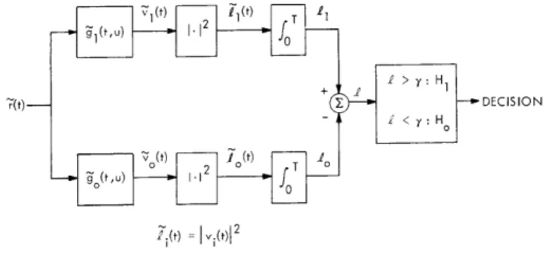
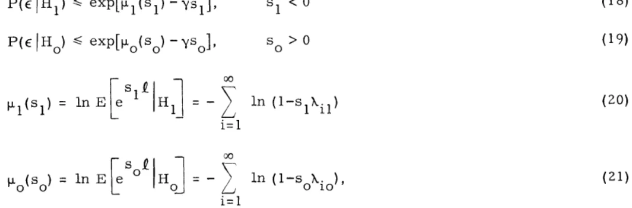
The receivers of Figs. XVIII-5, XVIII-6, and XVIII-7 fall into the class treated by Collins and Kurth in Section XVIII-C. Bounds on the error probabilities for the receiver of Fig. XVIII-5 are

P(E IH₁) < exp[l(sl) - ysl], s1 <0 (18)

P(E IH) < exp[ (s0o) - YSo] s > 0 (19)

I1(S1) = In Ee H1 = - In (l-slil) (20)

i=l

o(so) = in E

e

H = - In (1-sokXio)' (21)

i=l

where f is indicated in Fig. XVIII-5, and the Xij are the eigenvalues of the complex random process £l(t) - o (t) under hypothesis j,j = 0, 1. The bounds above and those of Eq. 9 permit a comparison of the optimum and suboptimum detectors. Evalua-tion of the bounds is feasible where the representaEvalua-tions of Figs. XVIII-6 or XVIII-7 are used. The procedure is outlined below for a special case.

For the equilikely binary orthogonal communication problem of Eq. 5, the thresh-old y in Eqs. 18 and 19 is zero, and the bound on the probability of error becomes

where

~l(sl)

= In E

e

s₁(f₁

-o)

_H1

= n E Ees1 H] E[e-s1 o H1

[ln (1-sXlis) + ln(1+sXlin)],

-[max

kin

] -

_{1 < s}

I

< 0.

i

The .is and

X.in

are

is in

H1. Since fl(t) and The expression have state-variable on the right side of

7 as

the eigenvalues of the processes Pl(t) and Jo(t) in Fig. XVIII-5, under f2(t) are orthogonal, ll(t) and ko (t) are independent.

for _{l(s) in Eq. 23 can be evaluated when the processes f1 and f (t} ) representations, as in Figs. XVIII-6 and XVIII-7. The first term Eq. 23 is related to a Fredholm determinant and can be expressed

ln (1-slis.

) = n det

21(0, T)

P +0

2(0

i=l1

where 021(0, T) and 022(0, T) are partitions of the transition matrix satisfying

_Fc(t)

de(t, T)

dt

4---F (t)

O(T, T) = I. (25b)

Under H1 the input to the receiver branch containing l(t) is s(t) + n(t). Thus the com-posite matrices F c(t), Gc (t), 9c, C (t), and Pc are those for the system shown in Fig. XVIII-6, with i = 1. If the state vectors x (t) and Y (t) are adjoined, these matrices are F I 0 F (t) = -- ---c

f(t) B(t) C

A(t)

G c(t) =

I

0

I(t)

(26)

(27)

00

il

i=1

(23) (24) 0(t, 7).

(25a)

,T) + Tr

_[F

_{c(t)] dt]}

C (t) = O I H(t) (28) Q 0

Q

=

(29)

- No P P - --- (30) -c 0 I

The subscripts in Fig. XVIII-6 have been ignored above.

The second term in Eq. 23 is computed in a similar manner. In Eqs. 24 and 25 the sign of sI is reversed, and the composite matrices of Eqs. 26-30 reduce to just those

of the receiver portion of Fig. XVIII-6. This is because under H1 the input to the 0th branch of the demodulator is just w(t).

The special case of Fig. XVIII-7 is included in the preceding discussion. The opti-mum and suboptiopti-mum performances now can be contrasted by minimizing [1(sl) over s I and comparing it with c(1/2) from Eq. 12.

4. Examples

In the following examples the performance of the suboptimum receiver of Fig. XVIII-7 for the binary symmetric communication problem of Eq. 5 is compared with the optimum performance. The exponent 1 1( 1) of Eq. 23 is minimized over sl. The exponent for the optimum receiver is

p

c(1/2) in Eq. 12.

The first case to be treated comprises a first-order Butterworth fading spectrum and a transmitted signal with a constant envelope. The spectrum is

2kP b(W) = _b 22_{+ k}2

and

f(t) =, 0 _< t-< T.

The average received energy in the signal component is E = EtP.

r

t

This spectrum implies that the receiver of Fig. XVIII-8 is of the form

Fig. XVIII-8.

Probability of error exponent for optimum and suboptimum receivers.

14I.I

Fig. XVIII-9. Pulse train.

Table XVIII-1. Performance comparison for pulse train with first-order

Butterworth fading.

Er/No

N

d

()

min I (S 1)

kr/k

10

3

.1

-1.42

-1.41

3

10

3

.5

-1.26

-1.25

2.5

30

8

.1

-4.21

-4.17

6

_

I I I I I

I

A -pc(1/2), OPTIMUM KT B-min J,(S1)_, OPTIMUM KT C -pc(1/2), 1/10 OPTIMUM KT D- min pl(S1), 1/10 OPTIMUM KT C

A-Figure XVIII-8 shows ic(1/2) and t1(S1) versus Er/No for two choices of the product kT. First, kT is chosen to minimize c(1/2) at each Er/No. Then krT is picked to optimize 1( 1). The second set of curves is for kT equal to 1/10 of the optimum value at each Er/No . The curves of Fig. XVIII-8 show that the "optimized" suboptimum receiver of Fig. XVIII-7 achieves a performance within 0. 5 dB of the optimum for Er/No greater than one. Although it is not indicated, the value of k T which maximizes the performance of the suboptimum scheme for large Er/No (large kT) is close to that pre-dicted by Eq. 15. With regard to the bound of Eq. 13, the receiver exponent C(1/2) never exceeds 0. 121 (Er/No) in Fig. XVIII-8.

A somewhat better signal for the one-pole fading spectrum is the pulse train of Fig. XVIII-9. It consists of N square pulses each with duty cycle d. The exponent

Lc(1/2) is minimized when N is approximately equal to the optimum kT at any given Er/No, and d is made as small as possible, subject to the transmitter peak-power con-straint. The resulting magnitude of

pc

(1/2) is bounded by 0. 142 Er/No. Table XVIII-1 gives a comparison of c (1/2) with l(s ₁) for some representative signal-to-noise ratios. Given E /N and d, N and kT are chosen to approximately minimize e(1/2), and then krT is adjusted to optimize il(sl). The suboptimum receiver performs nearly as well as the optimum receiver with these parameter values. The value of the optimum-time constant, krT, is consistent with a diversity interpretation of the signal of Fig. XVIII-9. In such a case the optimum receiver correlates only over the duration of each component pulse and sums the squares of the correlator outputs. Hence k rT is of the order of N • kT and the summation is approximated by the integrator following the squarer in Fig. XVIII-7.

The performance comparison for a second-order Butterworth fading spectrum has been carried out for the two signals used above. The results are not presented here, but they are similar to those of Fig. XVIII-8 and Table XVIII-1.

5. Summary

A suboptimum receiver has been analyzed for the detection of known signals trans-mitted over a Gaussian, Doppler-spread channel and received in additive Gaussian white noise. The form of the receiver is suggested by the structure of the optimum

filter-squarer detector in several limiting cases. Bounds on the error probabilities for the suboptimum receiver have been presented and compared with the performance of the optimum receiver in several examples. For the signals and spectra evaluated, the sub-optimum receiver performance is close to sub-optimum when the system parameters are appropriately chosen.

References

1. H. L. Van Trees, Detection, Estimation, and Modulation Theory, Part II (John

Wiley and Sons, Inc., New York, 1968).

2.

L. D. Collins, "Asymptotic Approximations to the Error Probability for Detecting

Gaussian Signals," Sc. D. Thesis, Department of Electrical Engineering, M. I. T.

June 1968.

3.

R. S. Kennedy, Private communication, 1968.

4.

J. N. Pierce, "Approximate Error Probabilities for Optimal Diversity Combining,"

IRE Trans.

,

Vol. CS-11, pp. 352-353, September 1963.

5.

R. Price and P. E. Green, Jr., "Signal Processing in Radar Astronomy -

Communi-cation via Fluctuating Multipath Media," Technical Report 234, Lincoln Laboratory,

M. I. T. , October 1960.

6.

A. B. Baggeroer, L. D. Collins, and H. L. Van Trees, "Complex State Variables:

Theory and Applications," a paper to be presented at WESCON, Los Angeles,

Cali-fornia, August 20-23, 1968.

7.

A. B. Baggeroer, "A State-variable Approach to the Solution of Fredholm Integral

Equations," Technical Report 459, Research Laboratory of Electronics, M. I. T. ,

Cambridge, Massachusetts, November 15, 1967.