Linear Total Variation Approximate Regularized Nuclear Norm Optimization for Matrix Completion

(1)

HAL Id: inserm-01101215

https://www.hal.inserm.fr/inserm-01101215

Submitted on 26 May 2015

HAL is a multi-disciplinary open access

archive for the deposit and dissemination of

sci-entific research documents, whether they are

pub-lished or not. The documents may come from

teaching and research institutions in France or

abroad, or from public or private research centers.

L’archive ouverte pluridisciplinaire HAL, est

destinée au dépôt et à la diffusion de documents

scientifiques de niveau recherche, publiés ou non,

émanant des établissements d’enseignement et de

recherche français ou étrangers, des laboratoires

publics ou privés.

Linear Total Variation Approximate Regularized

Nuclear Norm Optimization for Matrix Completion

Xu Han, Jiasong Wu, Lu Wang, Yang Chen, Lotfi Senhadji, Huazhong Shu

To cite this version:

Xu Han, Jiasong Wu, Lu Wang, Yang Chen, Lotfi Senhadji, et al.. Linear Total Variation Approximate

Regularized Nuclear Norm Optimization for Matrix Completion. Abstract and Applied Analysis,

Hindawi Publishing Corporation, 2014, 2014, pp.765782. �10.1155/2014/765782�. �inserm-01101215�

(2)

Research Article

Linear Total Variation Approximate Regularized Nuclear Norm

Optimization for Matrix Completion

Xu Han,

1,2

Jiasong Wu,

1,2,3,4

Lu Wang,

2,3,4

Yang Chen,

1,2,3

Lotfi Senhadji,

2,3,4

and Huazhong Shu

1,2

1_{Laboratory of Image Science and Technology, Southeast University, Nanjing 210096, China} 2_{Centre de Recherche en Information M´edicale Sino-franc¸ais (CRIBs), France}

3_{INSERM, U1099, Rennes 35000, France}

4_{Universit´e de Rennes 1, LTSI, Rennes 35042, France}

Correspondence should be addressed to Xu Han; [email protected] Received 15 February 2014; Accepted 7 May 2014; Published 28 May 2014 Academic Editor: Zhiwu Liao

Copyright © 2014 Xu Han et al. This is an open access article distributed under the Creative Commons Attribution License, which permits unrestricted use, distribution, and reproduction in any medium, provided the original work is properly cited.

Matrix completion that estimates missing values in visual data is an important topic in computer vision. Most of the recent studies focused on the low rank matrix approximation via the nuclear norm. However, the visual data, such as images, is rich in texture which may not be well approximated by low rank constraint. In this paper, we propose a novel matrix completion method, which combines the nuclear norm with the local geometric regularizer to solve the problem of matrix completion for redundant texture images. And in this paper we mainly consider one of the most commonly graph regularized parameters: the total variation norm which is a widely used measure for enforcing intensity continuity and recovering a piecewise smooth image. The experimental results show that the encouraging results can be obtained by the proposed method on real texture images compared to the state-of-the-art methods.

1. Introduction

The problem of matrix completion, which can be seen as the extension of recently developed compressed sensing (CS) theory [1–3], plays an important role in the field of signal and image processing [4–11]. This problem occurs in many real applications in computer vision and pattern recognition, such as image inpainting [12,13], video denoising [14], and recommender systems [15, 16]. Reconstruction algorithms for matrix completion have received much attention. Cai et al. [17] proposed an algorithm, namely, the singular value thresholding (SVT) algorithm for matrix completion and related nuclear norm minimization problems. In [18], a simple and fast singular value projection (SVP) algorithm for rank minimization with affine constraints is exploited. Keshavan et al. [19] dealt with the matrix completion based on singular value decomposition followed by local manifold optimization. In order to achieve a better approximation of the rank of matrix, Hu et al. [11] presented an approach based on the truncated nuclear norm regularization (TNNR), which is defined by the difference between the nuclear norm

and the sum of the largest few singular values. Since most of the existing matrix completion models aim to solve the low rank optimization via nuclear norm, we recall here this model. For an incomplete matrixM ∈ R𝑚×𝑛of rank𝑟, the model can be described as follows:

min

X rank(X) s.t. XΩ= MΩ, (1)

whereX ∈ R𝑚×𝑛andM_Ω = M_𝑖𝑗, (𝑖, 𝑗) ∈ Ω, and Ω is the set of locations corresponding to the observed entries.

Unfortunately, the rank minimization problem in (1) is an NP-hard one, so the following convex relaxation is widely used:

min

X ‖X‖∗ s.t. XΩ= MΩ, (2)

where‖ ⋅ ‖_∗is the nuclear norm given by ‖X‖∗ =

min(𝑚,𝑛)

∑

𝑘=1

𝜎_𝑘, (3)

where𝜎_𝑘denotes the𝑘th largest singular value of X.

Volume 2014, Article ID 765782, 8 pages http://dx.doi.org/10.1155/2014/765782

(3)

2 Abstract and Applied Analysis

In this paper, our objective is to exploit the intrinsic geometry of the data distribution and incorporate it as an additional regularization term to deal with the images which are rich in texture. The total variation (TV) norm has demonstrated its usefulness as a graph regularizer in the field of image processing, so we propose here a method that combines the nuclear norm with the linear TV approximate norm to solve the problem of matrix completion. We call it the linear total variation approximate regularized nuclear norm (LTVNN) minimization problem. This combination optimization problem will be solved by simple and efficient optimization scheme based on the alternating direction method of multipliers (ADMM) model [20,21].

The paper is organized as follows. In the next section, we introduce the proposed LTVNN model and we describe the optimization schemes. In Section 3, we establish the convergence results for the iterations given in Section 2. Experimental results on a set of images are provided in

Section 4. Finally, we draw some conclusions inSection 5.

2. Proposed Method

2.1. Some Preliminaries. The total variation along the vertical

and horizontal directions can be described as

𝐷V

𝑗,𝑘(X) = {X_0,𝑗,𝑘− X𝑗+1,𝑘, 1 ≤ 𝑗 < 𝑚_{𝑗 = 𝑚,} (4)

𝐷ℎ

𝑗,𝑘(X) = {X_0,𝑗,𝑘− X𝑗,𝑘+1, 1 ≤ 𝑘 < 𝑛_{𝑘 = 𝑛.} (5)

So the total variation ofX is the summation for the magnitude of the gradient of each pixel [22]:

‖X‖TV= ∑ 𝑗,𝑘 √(𝐷V 𝑗,𝑘X) 2 + (𝐷ℎ 𝑗,𝑘X) 2 . (6)

And the equvalent total variation formula as follows:

‖X‖TV= ∑ 𝑗,𝑘(󵄨󵄨󵄨󵄨󵄨𝐷

V

𝑗,𝑘X󵄨󵄨󵄨󵄨󵄨 +󵄨󵄨󵄨󵄨_󵄨𝐷ℎ𝑗,𝑘X󵄨󵄨󵄨󵄨󵄨). ₍₇₎

Here, we use the linear total variation approximate of (7) to approximate the second kind of total variation; that is,

‖X‖LTVA= ∑ 𝑗,𝑘 ((𝐷V 𝑗,𝑘X) 2 + (𝐷ℎ_𝑗,𝑘X)2) . ₍₈₎

2.2. Proposed Model. As mentioned above, the key point of

the proposed approach is the combination of the nuclear norm and the linear total variation approximate norm; therefore, the optimization problem is described as

min

X (1 − 𝛾) ‖X‖∗+ 𝛾‖X‖LTVA s.t. XΩ= MΩ, (9)

where0 ≤ 𝛾 ≤ 1 is a penalty parameter, ‖X‖_∗is the nuclear norm defined in (3), and ‖X‖LTVA is linear total variation

norm approximate defined in (8), which can be reformulated as

‖X‖LTVA= Tr [(X − X𝜙1) (X − X𝜙1)𝑇]

+ Tr [(X − 𝜙₂X) (X − 𝜙₂X)𝑇] = 󵄩󵄩󵄩󵄩(X − X𝜙1)󵄩󵄩󵄩󵄩2𝐹+ 󵄩󵄩󵄩󵄩(X − 𝜙2X)󵄩󵄩󵄩󵄩2𝐹,

(10)

where “Tr” means the trace of the matrix,‖ ⋅ ‖_𝐹denotes the Frobenius norm of the matrix, and𝜙₁and𝜙₂are, respectively, the column and row transform matrix given by

𝜙1= [ [ [ [ [ [ [ [ [ 0 0 0 ⋅ ⋅ ⋅ 0 1 0 ⋅ ⋅ ⋅ 0 0 1 0 0 .. . ... d ... 0 0 ⋅ ⋅ ⋅ 1 ⏟⏟⏟⏟⏟⏟⏟⏟⏟⏟⏟⏟⏟⏟⏟⏟⏟⏟⏟⏟⏟ (𝑛−1)×(𝑛−1) 0 0 .. . 1 ] ] ] ] ] ] ] ] ]𝑛×𝑛 , 𝜙₂= [ [ [ [ [ [ [ [ [ [ [ (𝑚 − 1) × (𝑚 − 1) 0 ⏞⏞⏞⏞⏞⏞⏞⏞⏞⏞⏞⏞⏞⏞⏞⏞⏞⏞⏞⏞⏞1 0 ⋅ ⋅ ⋅ 0 0 0 1 0 0 0 .._. .._{. d} .._. .. . 0 0 ⋅ ⋅ ⋅ 1 0 0 0 ⋅ ⋅ ⋅ 1 ] ] ] ] ] ] ] ] ] ] ]𝑚×𝑚 . (11)

So, the problem in (9) can be rewritten as min X (1 − 𝛾) ‖X‖∗+ 𝛾󵄩󵄩󵄩󵄩(X − X𝜙1)󵄩󵄩󵄩󵄩 2 𝐹 + 𝛾󵄩󵄩󵄩󵄩(X − 𝜙2X)󵄩󵄩󵄩󵄩2𝐹 s.t. X_Ω= M_Ω. (12)

2.3. The Optimization Scheme. The alternating direction

method of multipliers-ADMM [20, 21] is an efficient and scalable optimization model which exploits the structure of the optimization problem. In this section, we use ADMM to deal with the problem in (12), which can be reformulated as

min X,W(1 − 𝛾) ‖X‖∗+ 𝛾󵄩󵄩󵄩󵄩(W − W𝜙1)󵄩󵄩󵄩󵄩 2 𝐹 + 𝛾󵄩󵄩󵄩󵄩(W − 𝜙2W)󵄩󵄩󵄩󵄩2𝐹 s.t. X = W, W_Ω= M_Ω, (13)

where ‖(W − W𝜙₁)‖2_𝐹 and ‖(W − 𝜙₂W)‖2_𝐹 are the indicator functions. The augmented Lagrange function of (13) is

L (X, Y, W, 𝜆) = (1 − 𝛾) ‖X‖∗+ 𝛾󵄩󵄩󵄩󵄩(W − W𝜙1)󵄩󵄩󵄩󵄩2𝐹

+ 𝛾󵄩󵄩󵄩󵄩(W − 𝜙2W)󵄩󵄩󵄩󵄩2𝐹+𝜆₂‖W − X‖2𝐹

+ Tr (Y𝑇(W − X)) ,

(14)

where𝜆 > 0 is the penalty parameter and Y is the multiplier. The solution can be obtained by incorporating the solutions

(4)

of each regularization problem separately which are defined as follows. Row TV is as follows: L_𝑅(XR, YR, WR, 𝜆) = (1 − 𝛾) ‖XR‖∗+ 𝛾󵄩󵄩󵄩󵄩(WR − 𝜙2WR)󵄩󵄩󵄩󵄩2𝐹 +𝜆 2‖WR − XR‖2𝐹+ Tr (YR𝑇(WR − XR)) , (15)

whereXR denotes the optimization result along the vertical direction of the total variation defined in (4).

Column TV is as follows: L_𝐶(XC, YC, WC, 𝜆)

= (1 − 𝛾) ‖XC‖∗+ 𝛾󵄩󵄩󵄩󵄩(WC − WC𝜙1)󵄩󵄩󵄩󵄩2𝐹

+𝜆₂‖WC − XC‖2_𝐹+ Tr (YC𝑇(WC − XC)) , (16)

whereXC denotes the optimization result along the horizontal direction of the total variation defined in (5).

We deal with column linear TV optimization problem in (16) by the following steps in each iteration.

Step 1 (initial setting). XC₁ = M_Ω,WC₁= XC₁,YC₁ = XC₁,

with the tolerance𝜀.

Step 2 (computingXC_𝑘+1). FixWC_𝑘andYC_𝑘, and minimize

(16) for obtainingXC_𝑘+1as XC_𝑘+1= arg min X (1 − 𝛾) ‖XC‖∗+ 𝛾󵄩󵄩󵄩󵄩(WC𝑘− WC𝑘𝜙1)󵄩󵄩󵄩󵄩 2 𝐹 +𝜆₂󵄩󵄩󵄩󵄩WC − XC_𝑘󵄩󵄩󵄩󵄩2_𝐹+ Tr (YC𝑇_𝑘(WC − XC_𝑘)) . (17) Ignoring the constant terms, (17) can be rewritten as

XC_𝑘+1= arg min X (1 − 𝛾) ‖XC‖∗ +𝜆 2󵄩󵄩󵄩󵄩󵄩󵄩󵄩XC − (WC𝑘+ 1 𝜆YC𝑘)󵄩󵄩󵄩󵄩󵄩󵄩󵄩 2 𝐹. (18)

To solve (18), Cai et al. [17] introduce the soft-thresholding operatorD_𝜏which is defined as follows:

D_𝜏(X) := UD𝜏(Σ) V𝑇,

D_𝜏(Σ) = diag {max (𝜎_𝑖− 𝜏)₊} , (19) where𝑡₊= max(0, 𝑡).

Using the operatorD_𝜏in (19), the solution of (18) can be obtained as

XC𝑘+1= D(1−𝛾)/𝜆(WC𝑘+_𝜆1YC𝑘) . (20)

Step 3 (computingWC_𝑘+1). FixXC_𝑘+1andYC_𝑘and calculate

WC_𝑘+1as follows:

WC_𝑘+1= arg min

W L (XC𝑘+1, YC𝑘, WC, 𝜆) (21)

which is a quadratic function ofWC and can be easily solved by setting the derivation ofL(XC_𝑘+1, YC_𝑘, WC, 𝜆) to zeros, and then we get

WC_𝑘+1= (𝜆XC_𝑘+1− YC_𝑘)

× [2𝛾 (I − 𝜙₁− 𝜙𝑇₁ + 𝜙𝑇₁𝜙₁) + 𝜆I_𝑛×𝑛]−1. (22) Then we fix the values at the observed entries:

WC𝑘+1= (WC𝑘+1)Ω𝑚+ MΩ, (23)

whereΩ_𝑚denotes the set of the missing entries.

Step 4 (computingYC_𝑘+1). FixXC_𝑘+1andWC_𝑘+1and

calcu-lateYC_𝑘+1as follows:

YC_𝑘+1= YC_𝑘+ 𝜆 (WC_𝑘+1− XC_𝑘+1) . (24) Until the stop condition:‖XC_𝑘+1− XC_𝑘‖_𝐹≤ 𝜀.

Row TV problem defined by (15) can be solved in a similar way to that of column TV problem. The only difference is the

WR_𝑘+1in the second step, which is given by

WR_𝑘+1= [2𝛾 (I − 𝜙₂− 𝜙𝑇

2 + 𝜙2𝑇𝜙2) + 𝜆I𝑚×𝑚]−1

× (𝜆XR𝑘+1− YR𝑘) .

(25)

And the stop condition is‖XR_𝑘+1− XR_𝑘‖_𝐹≤ 𝜀.

Finally, we obtainedX_𝑘+1 as the average of XC_𝑘+1 and

XR𝑘+1; that is,

X_𝑘+1= XC𝑘+1+ XR₂ 𝑘+1. (26)

3. Convergence Analysis

In this section, we give the proof of the convergence of column total variation (16) and the convergence of row total variation is similar to the column total variation. Here, the objection function (16) about column variation is as follows:

min X 𝑓𝜏(X) s.t. X_Ω= M_Ω 𝑓_𝜏(X) = 𝜏‖X‖_∗+1 2Tr[(X − X𝜙1) (X − X𝜙1) 𝑇_{] ,} 𝜏 = 1 − 𝛾 2𝛾 . (27)

Lemma 1. Let Z ∈ 𝜕𝑓_𝜏(X) and Z󸀠∈ 𝜕𝑓_𝜏(X󸀠). Then

⟨Z − Z󸀠, X − X󸀠_{⟩ ≥ 󵄩󵄩󵄩󵄩󵄩X − X}󸀠󵄩󵄩󵄩󵄩_󵄩2_𝐹. (28)

(5)

(a) Original image (256× 256) (b) Random masked image (c) 𝛾 = 0, PSNR: 8.934

(d)𝛾 = 0.5, PSNR: 29.183 (e)𝛾 = 1, PSNR: 8.593 (f) Word masked image

(g)𝛾 = 0, PSNR: 14.706 (h)𝛾 = 0.5, PSNR: 33.421 (i) 𝛾 = 1, PSNR: 14.759

Figure 1: The recovered results with 60% random mask and word mask for𝛾 = 0, 0.5 and 1 by LTVNN.

Theorem 2. Assuming that the sequence of step size obeys

0 < inf 𝜆_𝑘 < sup 𝜆_𝑘 < (2𝛼/𝛽), 𝛼 = ⟨(X𝑘 _{− X}∗_{)(I − 𝜙} 1−

𝜙𝑇

1 + 𝜙1𝜙1𝑇), X𝑘− X∗⟩ and 𝛽 = ‖X𝑘− X∗‖ 2

𝐹. Here,X∗denotes

the optimization result andX𝑘denotes the𝑘th iteration object

variable; then by the iteration procedure defined inSection 2.3,

we can obtain the unique optimization result, that is,X∗. And

the details of the proof can be found in the Appendix.

4. Experiments

In this section, we test the proposed method on a set of images. The algorithm was implemented with MATLAB programming language on a PC machine, which sets up

Microsoft Windows 7 operating system and has an Intel Core I5 CPU with speed of 2.79 GHz and 2 GB RAM.

We deal with three channels (𝑟, 𝑔, 𝑏) of color images separately and combine the results together to get the final outcome. We use peak signal-to-noise ratio (PSNR) values to evaluate the performance:

PSNR= 10 × log₁₀(255

2

MSE) , (29)

where MSE denotes mean squared error,

MSE= 1

(6)

0 0.1 0.2 0.3 0.4 0.5 0.6 0.7 0.8 0.9 1 40 35 30 25 20 15 10 5 PS NR 40% sample 50% sample 60% sample 70% sample 80% sample 90% sample Word mask sample 𝛾 value

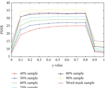
Figure 2: The recovered PSNR for Pepper under different random sample ratio and word mask sample with𝛾 from 0 0 to 1 by LTVNN.

0.4 0.5 0.6 0.7 0.8 0.9 36 34 32 30 28 26 24 22 20 18 PS NR LTVNN TNNR SVT SVP OptSpace Sampled ratio under 𝛾 = 0.5

Figure 3: Recovered PSNR for Pepper under𝛾 = 0.5 with different random sample ratio by LTVNN, TNNR, SVT, SVP, and OptSpace.

In the experiments, we consider two situations: random mask sample and word mask sample.Figure 1describes the recovered results with 60% random mask and word mask for 𝛾 = 0, 0.5 and 1 by LTVNN.Figure 2shows the recovered PSNR for Pepper under different random sample ratios and word mask sample for 𝛾 from 0 to 1 with step of 0.1 by LTVNN. It can be observed from these two figures that the best result is obtained for the value of𝛾 near to 0.5, which corresponds to the case where the two norms (nuclear and LTV) are equivalently used in (9). For the two extreme cases: 𝛾 = 0 (only the nuclear norm is taken into consideration) and𝛾 = 1 (only the linear total variation approximate norm is considered), the algorithm loses its efficiency.

We also compare our method (LTVNN) with other matrix completion methods including TNNR [10,11], SVT [12], SVP [13], and OptSpace [14].Figure 3plots the recovered PSNR for Pepper for𝛾 = 0.5 with different random sample ratios (from 40% to 90%) by LTVNN and other four methods (TNNR, SVT, SVP, and OptSpace). It can be seen from

Figure 3that the proposed LTVNN method achieves much higher PSNR than the other methods. Figure 4 shows the comparison of PSNR of recovered methods for Lena under word mask with𝛾 = 0.5 by LTVNN and the other methods.

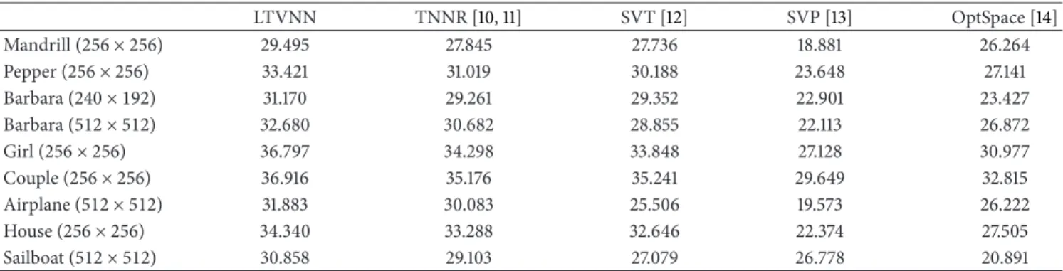
Table 1lists the PSNR results under word mask sample with 𝛾 = 0.5 for different images by LTVNN and the other methods. From Figure 4 and Table 1, we can see that the proposed method outperforms the other matrix completion methods under word mask for different images.

5. Conclusion

In this paper, we have proposed a new model that combines the nuclear norm and total variation norm for the matrix completion problem, which was then solved by ADMM model. Experimental results demonstrate the effectiveness of the proposed algorithm compared to other methods.

Appendix

Before we give the proof ofTheorem 2, we supplement one proof about

⟨(X − X󸀠) (I − 𝜙₁− 𝜙₁𝑇+ 𝜙₁𝜙₁𝑇) , X − X󸀠⟩ ≥ 0. (A.1) Without loss of generality, we take an example matrix𝜉 = (X − X󸀠_{) ∈ R}4×4_{and the corresponding transform matrix}

(I − 𝜙₁− 𝜙𝑇 1 + 𝜙1𝜙𝑇1) = [ 2 −1 0 0 −1 2 −1 0 0 −1 2 0 0 0 0 0]. Then, Tr[(Ι − 𝜙₁− 𝜙𝑇₁ + 𝜙₁𝑇𝜙₁) 𝜉𝑇𝜉] = 2 (𝜉2_1,1+ 𝜉2_2,1+ 𝜉2_3,1+ 𝜉_4,12 ) − (𝜉_1,1𝜉_1,2+ 𝜉_2,1𝜉_2,2+ 𝜉_3,1𝜉_3,2+ 𝜉_4,1𝜉_4,2) + 2 (𝜉2_1,2+ 𝜉2_2,2+ 𝜉_3,22 + 𝜉_4,22 ) − (𝜉_1,1𝜉_1,2+ 𝜉_2,1𝜉_2,2+ 𝜉_3,1𝜉_3,2+ 𝜉_4,1𝜉_4,2) − (𝜉_1,2𝜉_1,3+ 𝜉_2,2𝜉_2,3+ 𝜉_3,2𝜉_3,3+ 𝜉_4,2𝜉_4,3) + 2 (𝜉2_1,3+ 𝜉2_2,3+ 𝜉_3,32 + 𝜉_4,32 ) − (𝜉_1,2𝜉_1,3+ 𝜉_2,2𝜉_2,3+ 𝜉_3,2𝜉_3,3+ 𝜉_4,2𝜉_4,3) = (𝜉2_1,1+ 𝜉_2,12 + 𝜉_3,12 + 𝜉_4,12 ) + (𝜉_1,1− 𝜉_1,2)2 + (𝜉_2,1− 𝜉_2,2)2+ (𝜉_3,1− 𝜉_3,2)2+ (𝜉_4,1− 𝜉_4,2)2 + (𝜉_1,2− 𝜉_1,3)2+ (𝜉_2,2− 𝜉_2,3)2+ (𝜉_3,2− 𝜉_3,3)2 + (𝜉_4,2− 𝜉_4,3)2+ (𝜉2 1,3+ 𝜉22,3+ 𝜉3,32 + 𝜉4,32 ) ≥ 0, (A.2)

(7)

(a) Original image (256× 256) (b) Word masked image (c) LTVNN (PSNR: 32.920)

(d) TNNR (PSNR: 30.189) (e) SVT (PSNR: 30.760) (f) SVP (PSNR: 22.159)

(g) OptSpace (PSNR: 26.492)

Figure 4: Comparison of PSNR of recovered methods for Lena under word mask with𝛾 = 0.5 by LTVNN, TNNR, SVT, SVP, and OptSpace.

Table 1: PSNR results under word mask sample with𝛾 = 0.5 for different images by LTVNN, TNNR, SVT, SVP, and OptSpace. LTVNN TNNR [10,11] SVT [12] SVP [13] OptSpace [14] Mandrill (256 × 256) 29.495 27.845 27.736 18.881 26.264 Pepper (256 × 256) 33.421 31.019 30.188 23.648 27.141 Barbara (240 × 192) 31.170 29.261 29.352 22.901 23.427 Barbara (512 × 512) 32.680 30.682 28.855 22.113 26.872 Girl (256 × 256) 36.797 34.298 33.848 27.128 30.977 Couple (256 × 256) 36.916 35.176 35.241 29.649 32.815 Airplane (512 × 512) 31.883 30.083 25.506 19.573 26.222 House (256 × 256) 34.340 33.288 32.646 22.374 27.505 Sailboat (512 × 512) 30.858 29.103 27.079 26.778 20.891

(8)

so the term⟨(X − X󸀠)(I − 𝜙₁− 𝜙𝑇₁ + 𝜙₁𝜙₁𝑇), X − X󸀠⟩ ≥ 0. The proof ofTheorem 2is as follows.

Proof. Let (X∗, Y∗) be primal-dual optimization for the

problem (27). The optimality conditions give

0 = Z𝑘− P_Ω(Y𝑘−1) ,

0 = Z∗− P_Ω(Y∗) , (A.3) whereZ𝑘 ∈ 𝜕𝑓_𝜏(X𝑘) and Z∗ ∈ 𝜕𝑓_𝜏(X∗). Then from (A.3), we deduce that

(Z𝑘− Z∗) − P_Ω(Y𝑘−1− Y∗) = 0 (A.4) and combine (A.4) withLemma 1that

⟨X𝑘− X∗, PΩ(Y𝑘−1− Y∗)⟩ = ⟨Z𝑘− Z∗, X𝑘− X∗⟩ ≥ ⟨(X𝑘− X∗) (Ι − 𝜙₁− 𝜙𝑇₁ + 𝜙₁𝑇𝜙₁) , X𝑘− X∗⟩ . (A.5) We observe (23) thatP_ΩX∗ = P_ΩW, 󵄩󵄩󵄩󵄩 󵄩PΩ(Y𝑘− Y∗)󵄩󵄩󵄩󵄩󵄩_𝐹 = 󵄩󵄩󵄩󵄩󵄩PΩ(Y𝑘−1− Y∗) + 𝜆𝑘PΩ(W − X𝑘)󵄩󵄩󵄩󵄩󵄩_𝐹 = 󵄩󵄩󵄩󵄩󵄩PΩ(Y𝑘−1− Y∗) + 𝜆𝑘PΩ(X∗− X𝑘)󵄩󵄩󵄩󵄩󵄩_𝐹. (A.6)

Here, we set𝑟_𝑘= ‖P_Ω(Y𝑘− Y∗)‖_𝐹; then 𝑟2 𝑘 = 𝑟𝑘−12 − 2𝜆𝑘⟨PΩ(Y𝑘−1− Y∗) , X𝑘− X∗⟩ + 𝜆2_𝑘󵄩󵄩󵄩󵄩_󵄩P_Ω(X∗− X𝑘_{)󵄩󵄩󵄩󵄩󵄩}2_𝐹 ≤ 𝑟_𝑘−12 − 2𝜆_𝑘⟨(X𝑘− X∗) (Ι − 𝜙₁− 𝜙𝑇₁ + 𝜙𝑇₁𝜙₁) , X𝑘− X∗⟩ + 𝜆2_𝑘󵄩󵄩󵄩󵄩_󵄩X𝑘− X∗󵄩󵄩󵄩󵄩_󵄩2_𝐹 = 𝑟_𝑘−12 − (2𝜆𝑘𝛼 − 𝜆2𝑘𝛽) , (A.7) where𝛼 = ⟨(X𝑘− X∗)(Ι − 𝜙₁− 𝜙𝑇₁ + 𝜙𝑇₁𝜙₁), X𝑘 − X∗⟩ ≥ 0, 𝛽 = ‖X𝑘_{− X}∗_‖2 𝐹≥ 0.

Based on (A.7), when(2𝜆_𝑘𝛼 − 𝜆2_𝑘𝛽) > 0, that is, 𝜆_𝑘 ∈ (0, 2𝛼/𝛽), the term ‖P_Ω(Y𝑘_{− Y}∗_)‖

𝐹 is nonincreasing and

converges to limit. The parameter𝜆_𝑘is very easy for satisfying this condition when𝜆_𝑘is smaller constant. And we can obtain other properties as follows.

Let𝜆_𝑘 = 𝛼/𝛽, and then 2𝜆_𝑘𝛼 − 𝜆2_𝑘𝛽 = 𝛼2/𝛽. Due to the fact that𝛼2/𝛽 converges to zero, so 𝛼2is infinite small about

𝛽 and converges to zero. Now we reconsider (A.2); evidently the first column in𝜉 converges to zero; that is, 𝜉_1,1 → 0, 𝜉_2,1 → 0, 𝜉_3,1 → 0, 𝜉_4,1 → 0. The second column converges to the first column and then converges to zero; that is,𝜉_1,2 → 𝜉1,1 → 0, 𝜉2,2 → 𝜉2,1 → 0, 𝜉3,2 → 𝜉3,1 → 0, 𝜉4,2 →

𝜉_4,1 → 0. The third column converges to the second column and then converges to zero; that is,𝜉_1,3 → 𝜉_1,2 → 0, 𝜉_2,3 → 𝜉_2,2 → 0, 𝜉_4,3 → 𝜉_4,2 → 0, 𝜉_1,2 → 𝜉_1,1 → 0, so through the iterationX𝑘converges toX∗except the last column due to the definition in (4) and (5); the last column and the last row are set to zero.

Fortunately, this problem does not have side effect for global result.Theorem 2is established.

Conflict of Interests

The authors declare that there is no conflict of interests regarding the publication of this paper.

Acknowledgments

This work was supported by the National Basic Research Pro-gram of China under Grant 2011CB707904, by the National Natural Science Foundation of China under Grants 61201344, 61271312, and 61073138, by the Ministry of Education of China under Grants 20110092110023 and 20120092120036, the Key Laboratory of Computer Network and Information Integration (Southeast University), Ministry of Education, and by Natural Science Foundation of Jiangsu Province under Grant BK2012329. This work is supported by INSERM postdoctoral fellowship.

References

[1] E. J. Cand`es, J. Romberg, and T. Tao, “Robust uncertainty principles: exact signal reconstruction from highly incomplete frequency information,” IEEE Transactions on Information

The-ory, vol. 52, no. 2, pp. 489–509, 2006.

[2] D. L. Donoho, “Compressed sensing,” IEEE Transactions on

Information Theory, vol. 52, no. 4, pp. 1289–1306, 2006.

[3] E. J. Cand`es, J. K. Romberg, and T. Tao, “Stable signal recovery from incomplete and inaccurate measurements,”

Communica-tions on Pure and Applied Mathematics, vol. 59, no. 8, pp. 1207–

1223, 2005.

[4] E. J. Cand`es and B. Recht, “Exact matrix completion via convex optimization,” Foundations of Computational Mathematics, vol. 9, no. 6, pp. 717–772, 2008.

[5] E. J. Cand`es and T. Tao, “The power of convex relaxation: near-optimal matrix completion,” IEEE Transactions on Information

Theory, vol. 56, no. 5, pp. 2053–2080, 2009.

[6] A. Eriksson and A. van den Hengel, “Efficient computation of robust low-rank matrix approximations in the presence of missing data using the L1 norm,” in Proceedings of the IEEE

Computer Society Conference on Computer Vision and Pattern Recognition (CVPR ’10), pp. 771–778, June 2010.

[7] H. Ji, C. Liu, Z. Shen, and Y. Xu, “Robust video denoising using Low rank matrix completion,” in Proceedings of the IEEE

Computer Society Conference on Computer Vision and Pattern Recognition (CVPR ’10), pp. 1791–1798, June 2010.

[8] J. Liu, P. Musialski, P. Wonka, and J. Ye, “Tensor completion for estimating missing values in visual data,” in Proceedings of the

IEEE 12th International Conference on Computer Vision (ICCV ’09), pp. 2114–2121, Kyoto, Japan, 2009.

[9] T. Okatani, T. Yoshida, and K. Deguchi, “Efficient algorithm for low-rank matrix factorization with missing components and

(9)

performance comparison of latest algorithms,” in Proceedings of

the IEEE International Conference on Computer Vision (ICCV ’11), pp. 842–849, Barcelona, Spain, November 2011.

[10] D. Zhang, Y. Hu, J. Ye, X. Li, and X. He, “Matrix completion by truncated nuclear norm regularization,” in Proceedings of the

IEEE Conference on Computer Vision and Pattern Recognition (CVPR ’12), pp. 2192–2199, 2012.

[11] Y. Hu, D. Zhang, J. Ye, X. Li, and X. He, “Fast and accurate matrix completion via truncated nuclear norm regularization,” IEEE

Transactions on Pattern Analysis and Machine Intelligence, vol.

35, no. 9, pp. 2117–2130, 2013.

[12] N. Komodakis and G. Tziritas, “Image completion using global optimization,” in Proceedings of the IEEE Conference on

Com-puter Vision and Pattern Recognition (CVPR ’06), vol. 1, pp. 442–

452, 2006.

[13] C. Rasmussen and T. Korah, “Spatiotemporal inpainting for recovering texture maps of partially occluded building facades,” in Proceedings of the IEEE International Conference on Image

Processing (ICIP ’05), vol. 3, pp. 125–128, September 2005.

[14] H. Ji, C. Liu, Z. Shen, and Y. Xu, “Robust video denoising using Low rank matrix completion,” in Proceedings of the IEEE

Conference on Computer Vision and Pattern Recognition (CVPR ’10), pp. 1791–1798, June 2010.

[15] Y. Koren, “Factorization meets the neighborhood: a multi-faceted collaborative filtering model,” in Proceedings of the

14th ACM SIGKDD International Conference on Knowledge Discovery and Data Mining, pp. 426–434, Las Vegas, Nev, USA,

August 2008.

[16] H. Steck, “Training and testing of recommender systems on data missing not at random,” in Proceedings of the 16th ACM

SIGKDD International Conference on Knowledge Discovery and Data Mining (KDD ’10), pp. 713–722, Washington, DC, USA,

July 2010.

[17] J.-F. Cai, E. J. Cand`es, and Z. Shen, “A singular value thresh-olding algorithm for matrix completion,” SIAM Journal on

Optimization, vol. 20, no. 4, pp. 1956–1982, 2010.

[18] P. Jain, R. Meka, and I. Dhillon, “Guaranteed rank minimization via Singular Value Projection,” in Proceedings of the 24th Annual

Conference on Neural Information Processing Systems (NIPS ’10),

Vancouver, Canada, December 2010.

[19] R. H. Keshavan, A. Montanari, and S. Oh, “Matrix completion from a few entries,” IEEE Transactions on Information Theory, vol. 56, no. 6, pp. 2980–2998, 2010.

[20] Z. Lin, R. Liu, and Z. Su, “Linearized alternating direction method with adaptive penalty for low-rank representation,” in

Proceedings of the 25th Annual Conference on Neural Informa-tion Processing Systems (NIPS ’11), December 2011.

[21] J. Yang and X. Yuan, “Linearized augmented Lagrangian and alternating direction methods for nuclear norm minimization,”

Mathematics of Computation, vol. 82, no. 281, pp. 301–329, 2013.

[22] L. I. Rudin, S. Osher, and E. Fatemi, “Nonlinear total variation based noise removal algorithms,” Physica D: Nonlinear

(10)

Submit your manuscripts at

http://www.hindawi.com

Hindawi Publishing Corporation

http://www.hindawi.com Volume 2014

Mathematics

Journal of

Mathematical Problems in Engineering

Hindawi Publishing Corporation http://www.hindawi.com

Differential Equations

International Journal of

Volume 2014 Hindawi Publishing Corporation

http://www.hindawi.com Volume 2014 Hindawi Publishing Corporationhttp://www.hindawi.com Volume 2014

Mathematical PhysicsAdvances in

Complex Analysis

Journal of Hindawi Publishing Corporation

Optimization

Journal of

Combinatorics

International Journal of Hindawi Publishing Corporation

Journal of

Function Spaces

Abstract and Applied Analysis Hindawi Publishing Corporation

http://www.hindawi.com Volume 2014 International Journal of Mathematics and Mathematical Sciences

Hindawi Publishing Corporation http://www.hindawi.com Volume 2014

The Scientific

World Journal

Discrete Dynamics in Nature and Society

Discrete Mathematics

Journal of

http://www.hindawi.com Volume 2014 Hindawi Publishing Corporationhttp://www.hindawi.com Volume 2014

Stochastic Analysis

International Journal of