PHASELESS DIFFRACTION TOMOGRAPHY WITH REGULARIZED BEAM PROPAGATION

PHASELESS DIFFRACTION TOMOGRAPHY WITH REGULARIZED BEAM PROPAGATION

Thanh-an Pham

, Emmanuel Soubies

, Joowon Lim

,

Alexandre Goy

,Ferr´eol Soulez

, Demetri Psaltis

, and Michael Unser

Biomedical Imaging Group, Ecole polytechnique f´ed´erale de Lausanne (EPFL), 1015 Lausanne, Switzerland

†_{Optics Laboratory, Ecole polytechnique f´ed´erale de Lausanne (EPFL), 1015 Lausanne, Switzerland}

‡_{Univ Lyon, Univ Lyon1, Ens de Lyon, CNRS, Centre de Recherche Astrophysique de Lyon UMR5574, F-69230, Saint-Genis-Laval, France.}

ABSTRACT

In recent years, researchers have obtained impressive reconstruc-tions of the refractive index (RI) of biological objects through the combined use of advanced physics (nonlinear forward model) and regularization. Here, we propose an adaptation of these techniques for the more challenging problem of intensity-only measurements. It involves a difficult nonconvex optimization problem where phase and distribution of the RI must be jointly estimated. Using an ad-equate splitting, we leverage recent achievements in phase retrieval and RI reconstruction to perform this task. This yields an efficient reconstruction method with sparsity constraints.

Index Terms— Beam propagation, intensity measurement, co-herence tomography, image reconstruction.

1. INTRODUCTION

Having access to the map of the refractive index (RI) of biological samples has a broad range of applications [1]. It can be obtained through optical diffraction tomography (ODT). There, the sample is illuminated by a set of tilted incident waves and holographic mea-surements of the resulting scattered fields are recorded (see Fig-ure 1). The RI distribution is then recovered by solving an inverse scattering problem.

Pioneering works to solve the recovery problem were relying on direct linear inversion algorithms such as back-propagation [2, 3]. Reconstructions were then dramatically improved using regularization-based methods [4, 5]. However, the validity of linear models is restricted to weakly scattering samples. To overcome this limita-tion, the most recent reconstruction algorithms combine advanced physical models with modern regularization [6, 7]. These methods account for multiple scattering, which opens the door to the imaging of strongly scattering objects.

As a CCD camera can measure intensity only, holographic mea-surements must be acquired using an elaborate interferometric setup that needs a reference beam or multiple measurements per angle. Phaseless diffraction tomography allows one to simplify this setup by recording a single intensity measurement per angle. However, this comes at the price of a more challenging inverse problem. Ex-isting methods tackle this difficulty by alternating between phase re-trieval and RI estimation. The phase estimation step is generally performed using the popular Gerchberg-Saxton projection [8]. The This research was supported by the European Research Council (ERC) under the European Union’s Horizon 2020 research and innovation pro-gramme, Grant Agreement no. 692726 “GlobalBioIm: Global integrative framework for computational bio-imaging.” Funding: European Research Council (ERC) (692726). δz n nb x z utot Sample Sensors (y ) uin 1 uinP Ω

Fig. 1. Diffraction-tomography setup. A sample of RI n = nb1 + δn

is immersed in a background medium of index nband impinged by a set of

incident waves (uin

p)p∈[1...P ]. The interaction of the wave with the object

produces a total field utot_{. Its squared magnitude is recorded by the detector.}

RI reconstruction step has known the same progression as for classi-cal ODT, going from linear models [9, 10] to nonlinear ones with ad hoc regularization [11, 12, 13].

Contributions In this paper, we propose phaseless diffraction to-mography as an adaptation of the efficient regularized method [6] that solves inverse scattering. We thereby leverage the benefit of an advanced nonlinear physical model and sparse regularization. We first express the inverse problem within a variational framework that includes the total variation (TV) penalty together with a nonnegativ-ity constraint. Then, using an adequate splitting strategy, we carry out the optimization by alternating between simpler steps. For each subproblem, we deploy an efficient numerical solution. Finally, we validate the proposed method on simulated and experimental data.

2. BEAM-PROPAGATION METHOD

We consider the 2D area Ω discretized in (Nx× Nz) points with steps δx and δz. We denote the RI distribution of the sample by n∈ RNx×Nz_{and the RI of the surrounding medium by n}

b∈ R. Also, we

introduce the RI variation δn = (n− nb1) with 1 =

∑NxNz

k=1 ek.

The incident plane wave of wavelength λ is referred to as uin ∈ CNx×Nz_{. We represent the total field u}tot_{(δn)∈ C}Nx×Nz_(incident + scattered) as

where a(δn) ∈ CNx×Nz _{is the complex envelope of the wave,} kb= 2πn_λb is the background wavenumber, and the index q denotes

the z slice of the corresponding matrix. The beam-propagation method (BPM) computes a(δn) slice-by-slice along the optical axis z using the recursive relation

aq(δn) = (aq−1(δn)∗ hprop)⊙ pq(δn), (2)

a0(δn) = uin0, (3)

where⊙ denotes the Hadamard product and ∗ the convolution op-eration. In (2), aq−1(δn) is first propagated to the next slice by convolution with the propagation kernel hprop∈ CNx_{given by}

hprop=F−1 { exp ( −jω2 δz kb+ √ kb2− ω2 )} (diffraction step), (4)

where F is the 1D discrete Fourier transform, ω ∈ RNx _is the frequency variable for the x direction, and all operations are component-wise. This convolution is followed by a point-wise mul-tiplication with the qth slice of the phase mask p(δn)∈ CN x×Nz defined as

pq(δn) = exp (jk0δz(δn)q) (refraction step), (5)

where k0 = kb/nb is the wavenumber in free space. Finally, the

BPM forward model is defined by the operator B : RNx×Nz → CNx δn 7→ aNz(δn) e jkbNz_, (6) where aNz(δn)∈ C Nx_{is computed using (2)-(3).} 3. ADMM-BASED RECONSTRUCTION We denote by P the number of the incident planes waves uin

p ∀ p ∈

[1 . . . P ]. The forward model that links δn to the intensity measure-ments yp∈ RNx is

yp=|Bp(δn)|2+ sp∀ p ∈ [1 . . . P ], (7)

where sp ∈ RNx is a vector of noise components, | · | denotes

the component-wise magnitude, (·)2 _{denotes the component-wise} square operation, and Bpis the BPM model in (6) associated to uinp.

To recover the RI variation δn, we minimize the TV-regularized neg-ative log-likelihood of the noise distribution

c δn∈ { arg min δn∈χ ( 1 2 P ∑ p=1 ∥|Bp(δn)|2− yp∥2Wp+ τ∥δn∥TV )} , (8)

with τ a regularization parameter, χ⊆ RNx×Nz

≥0 a set that enforces

the nonnegativity constraint, Wp = diag((wp1, . . . , w

p Nx)) ∈ RNx×Nx _{a diagonal matrix, and}∥ · ∥

Wa weighted ℓ2-norm such that∥v∥2W =

∑Nx

m=1w p

m(vm)2. To account for shot noise

(Pois-son), we set these weights to the inverse of the intensity of each measurement.

We then apply the popular alternating direction method of multi-pliers (ADMM) [14] strategy to solve our inverse problem. The lead-ing idea is to split the initial problem in a series of simpler subprob-lems for which we can deploy efficient algorithms. Starting from

Algorithm 1ADMM for minimizing (10)

Require: {yp}p∈[1...P ], δn(0)∈ RN≥0, ρ > 0, τ > 0

1: w(0)p = 0_CNx, ∀p ∈ [1 . . . P ] 2: k = 0

3: while(not converged) do 4: v(k+1)p = prox1 2ρ∥|·|2−yp∥2_Wp(Bp(δn (k) ) +w (k) p ρ ) 5: δn(k+1)= arg min δn∈χ ( 1 2 P ∑ p=1 ∥Bp(δn)− v(k+1)p + wp(k) ρ ∥ 2 2+ τ ρ∥δn∥TV ) 6: w(k+1)p = w(k)p +ρ(Bp(δn(k+1))−v(k+1)p ), ∀p ∈ [1 . . . P ] 7: k← k + 1 8: end while 9: return δn(k)

(8), we introduce the auxiliary variables vp ∈ CNx∀ p ∈ [1 . . . P ]

to obtain the equivalent constrained problem c δn∈ arg min δn∈χ ( 1 2 P ∑ p=1 ∥|vp|2− yp∥2Wp+ τ∥δn∥TV ) , s.t. vp= Bp(δn) ∀p ∈ [1 . . . P ]. (9)

This problem admits the augmented-Lagrangian form L(δn, v1, . . . , vP, w1, . . . , wP) = 1 2 P ∑ p=1 ∥|vp|2− yp∥2Wp +ρ 2∥Bp(δn)− vp+ wp/ρ∥ 2 2+ τ∥δn∥TV, (10) where wpand ρ are the Lagrangians and the penalty parameter [14].

Algorithm 1 shows the steps to minimize (10) using ADMM. 3.1. Proximity Operator

At Step 4 of Algorithm 1, one has to compute the proximity operator ofD(v) = 1

2ρ∥|v|

2_{− y}

p∥2Wpdefined as prox_D(x) = arg min

v∈CNx ( 1 2∥v − x∥ 2 2+D(v) ) . (11)

Here, we take advantage of the closed-form expressions that have been recently derived for both Gaussian and Poisson likelihoods in [15]. Specifically, the proximity operator in (11) is computed component-wise according to

∀x ∈ CNx_{, [prox}

D(x)]m= ϱme

jarg(xm)_{, (12)}

where ϱmis the positive root of the 3rd degree three polynomial

qG(ϱ) = 4wp m ρ ϱ 3 + ϱ ( 1−4w p m ρ [yp]m ) − |xm|, (13)

which is found with Cardano’s method. 3.2. Solving for δn

At Step 5 of Algorithm 1, we need to reconstruct the RI distribution from the complex “data” z(k+1)p = v(k+1)p − wp(k)/ρ, taking into

account that δn(k+1)= arg min δn∈χ ( 1 2 P ∑ p=1 ∥Bp(δn)−z(k+1)p ∥ 2 2+ τ ρ∥δn∥TV ) . (14)

This optimization problem is solved using the fast iterative shrinkage-thresholding algorithm (FISTA) [16], which has already been proven to be useful in this context [17, 6]. Two quantities are required

1. The proximity operator of τ

ρ∥ · ∥TVwhich is computed

effi-ciently using a standard iterative method [6].

2. The gradient of F(δn) = 1₂∑P_p=1∥Bp(δn)− z(k+1)p ∥22 which is derived using classical differential rules.

Specifically, we have that

∇F(δn) = P ∑ p=1 Re(JHBp(δn)(Bp(δn)− z (k+1) p ) ) , (15)

where JBp(δn) is the Jacobian matrix of the BPM forward model. It is computed efficiently by back-propagation as in [6].

Moreover, to reduce the computational cost, we compute the gradient only from a subset of angles L < P . We choose the an-gles such that they are equally spaced and increment them at each FISTA iteration. The computational complexity of∇F(δn) for one angle corresponds to the cost of 6NzFFTs of size Nx.

We implemented Algorithm 1 using the GlobalBioIm library [18].

4. NUMERICAL EXPERIMENTS 4.1. Simulated data

We simulated intensity measurements using a nonlinear accurate for-ward model [19]. The square area Ω = 33λ× 33λ includes the sample and the sensors. The medium has a RI nb= 1.33 (i.e.,

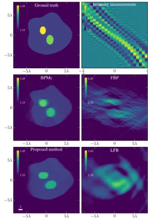
wa-ter). The setup is similar to the scheme in Figure 1. A cell-like phantom is included in a central area of side 16.5λ. As shown in Figure 2 (top left), the cell body and the two ellipses have a RI of 1.355, 1.432 and 1.457 respectively. We simulated on a very fine grid in order to reduce numerical errors (i.e., 1024× 1024) and then down-sampled (512× 512) to get the measurements used for the reconstruction (last column of this matrix). The plane waves have incident angles equally spaced between−π₄ and π₄. Thirty one sets of measurements were acquired with a wavelength of 406 nm (i.e., P = 31). The reconstruction problem is challenging because of the limited-angle illuminations (missing cone). We computed the recon-struction error∥δn−δntrue∥F

∥δntrue∥F with∥ · ∥F the Frobenius norm. Our reference is the (linear) light field refocusing (LFR) method [20] which is also used to initialize Algorithm 1. It provides a rea-sonably “good” start, which is crucial here since the optimization task is non-convex. The algorithm parameters were manually set to ρ = 10−3, L = 8 and the step size in FISTA to γ = 5· 10−4. Noiseless measurements For this experiment, we set the regular-ization parameter to τ = 1.5· 10−6· ∥yP /2∥22. We compare the

proposed method with the BPM method in [6] that reconstructs the RI map from holographic measurements (BPMc). We initialize this algorithm with a filtered back-projection method (FBP) [21]. As shown in Figure 2, the proposed method is able to recover the RI dis-tribution. One can observe that the structures are slightly elongated along z, as a consequence of the missing cone. However, contrar-ily to the LFR solution, we can distinguish the two ellipses and the shape of the cell body. The reconstructed RI is also close to the true value. The reconstruction error is 6· 10−3. The proposed method compares well against BPMc (error 5.4· 10−3) for which the phase was provided. 1.45 1.33 −5λ 0 5λ −5λ 0 5λ Ground truth 3 0 −π 4 0 π 4 Intensity measurements 1.45 1.33 −5λ 0 5λ −5λ 0 5λ BPMc 1.45 1.33 −5λ 0 5λ FBP 1.45 1.33 λ −5λ 0 5λ −5λ 0 5λ Proposed method _1.45 1.33 −5λ 0 5λ LFR

Fig. 2. Simulated data and their reconstruction. From left to right: (top) the cell-like phantom and its associated noiseless intensity measurements; (middle) the solutions from FBP [21] and BPMc [6]; (bottom) the LFR so-lution [20], and the RI distribution recovered by the proposed method. The elongated ellipses are due to missing informations along the optical axis.

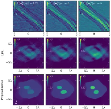
Noisy measurements We simulated noisy measurements at three different noise levels. For each of them, we set the incident fields (uinp)p∈[1...P ] such that |[uinp]m| = A ∈ R>0 and

simu-lated the resulting intensity measurements. We considered three scenarios with A = 1.75, 3 and 5. Then, these measurements were corrupted using a Poisson distribution. The resulting SNR are 5.32, 9.77 and 14.13 dB, respectively. Simulated measurements are shown in Figure 3 (top line). The regularizations were set to τ = 10−6· ∥yP /2∥22for all noise levels.

As shown in Figure 3 (bottom line), the proposed method is still able to recover the shape of the cell and the ellipses. The recon-struction errors are 9.47· 10−3, 8.07· 10−3 and 6.17· 10−3 for A = 1.75, 3 and 5, respectively. Despite the noise, we can still dis-tinguish the different elements of the phantom, which demonstrates the robustness of the method.

4.2. Experimental data

We validated our method on experimental data. Holographic mea-surements were collected using a standard Mach-Zehnder inter-ferometer, which relies on off-axis digital holography (λ = 450 nm). The sample was the cross-section of two fibres immersed in a medium of RI nb = 1.525 (oil). We obtained P = 160 views

ranging from−π

4 to

π

4. The RI variation is negative δn∈ R≤0. The reconstructed area is Ω = 38λ× 97λ. We compare the performance of the proposed method with BPMc. The latter and Algorithm 1 were

11 0 −π 4 0 π 4 |[uin p]m| = 1.75 27 0 −π 4 0 π 4 |[uin p]m| = 3 64 0 −π 4 0 π 4 |[uin p]m| = 5 1.45 1.33 −5λ 0 5λ −5λ 0 5λ LFR 1.45 1.33 −5λ 0 5λ 1.45 1.33 −5λ 0 5λ 1.45 1.33 λ −5λ 0 5λ −5λ 0 5λ Proposed method 1.45 1.33 −5λ 0 5λ 1.45 1.33 −5λ 0 5λ

Fig. 3. Noisy measurements and their RI reconstructions. Each col-umn corresponds to a noise level. From left to right: |[uin

p]m| = 1.75, |[uin

p]m| = 3, |[uinp ]m| = 5 ∀p ∈ [1 . . . P ]. Top to bottom: intensity

measurements, LFR [20], and proposed method.

initialized with the solutions of the Rytov based-backpropagation [3] and LFR respectively.

The FISTA step size was set at γ = 0.2/∥yP /2∥22 for BPMc and our method. We set the penalty parameter to ρ = 2.5 for Algo-rithm 1. The regularization parameter τ was tuned manually.

As shown in Figure 4, both BPMc and the proposed method are able to reconstruct the cross-section of the two fibres. Although the phase is missing, our method reaches performances similar to BPMc.

5. CONCLUSION

We have proposed a method to reconstruct a map of refractive in-dex (RI) from intensity-only measurements. It is a non-trivial exten-sion from complex to amplitude-only of a state-of-the-art method for RI reconstruction from holographic measurements. We have com-bined proximity operators for phase retrieval with an efficient RI re-construction pipeline. Using an adequate splitting of the problem, our method can cope with different noise models and regularizers. We showed its robustness to noise and to the limited-angle acquisi-tion settings that are the main difficulties for biological imaging.

6. REFERENCES

[1] D. Jin, R. Zhou, Z. Yaqoob, and P. T. C. So, “Tomographic phase microscopy: Principles and applications in bioimaging,” Journal of the Optical Society of America B, vol. 34, no. 5, pp. B64–B77, May 2017.

[2] E. Wolf, “Three-dimensional structure determination of semi-transparent objects from holographic data,” Optics Communications, vol. 1, no. 4, pp. 153–156, September 1969.

[3] A. J. Devaney, “Inverse-scattering theory within the Rytov approximation,” Optics Letters, vol. 6, no. 8, pp. 374–376, August 1981.

[4] Y. Sung, W. Choi, C. Fang-Yen, K. Badizadegan, R. R. Dasari, and M. S. Feld, “Optical diffraction tomography for high resolution live cell imaging,” Optics Express, vol. 17, no. 1, pp. 266–277, January 2009.

Measurements (194 λ ) 0 π 4 π 4 0 97λ -0.0563 0 Proposed BPMc BPMc Proposed ·10−2

Fig. 4. RI reconstructions of two fibres. Top left: profile plots of recon-structions from BPMc and proposed method of the dashed lines on the right. Bottom left: intensity measurements experimentally acquired. Right: BPMc (complex measurements) and proposed method (intensity measurements).

[5] J. Lim, K. Lee, K. Jin, S. Shin, S. Lee, Y. Park, and J. C. Ye, “Comparative study of iterative reconstruction algorithms for missing cone problems in optical diffraction tomography,” Optics Express, vol. 23, no. 13, pp. 16933–16948, June 2015.

[6] U. S. Kamilov, I. N. Papadopoulos, M. H. Shoreh, A. Goy, C. Vonesch, M. Unser, and D. Psaltis, “Optical tomographic image reconstruction based on beam propa-gation and sparse regularization,” IEEE Transactions on Computational Imaging, vol. 2, no. 1, pp. 59–70, January 2016.

[7] U. S. Kamilov, D. Liu, H. Mansour, and P. T. Boufounos, “A recursive Born approach to nonlinear inverse scattering,” IEEE Signal Processing Letters, vol. 23, no. 8, pp. 1052–1056, August 2016.

[8] R. Gerchberg and W. O. Saxton, “A practical algorithm for the determination of phase from image and diffraction plane pictures,” Optik, vol. 35, pp. 237, November 1972.

[9] G. Zheng, R. Horstmeyer, and C. Yang, “Wide-field, high-resolution Fourier pty-chographic microscopy,” Nature Photonics, vol. 7, no. 9, pp. 739–745, July 2013. [10] L. Tian, X. Li, K. Ramchandran, and L. Waller, “Multiplexed coded illumination for Fourier ptychography with an LED array microscope,” Biomedical Optics Express, vol. 5, no. 7, pp. 2376–2389, July 2014.

[11] A. M. Maiden, M. J. Humphry, and J. M. Rodenburg, “Ptychographic transmission microscopy in three dimensions using a multi-slice approach,” Journal of the Optical Society of America A, vol. 29, no. 8, pp. 1606–1614, August 2012. [12] L. Tian and L. Waller, “3D intensity and phase imaging from light field

measure-ments in an LED array microscope,” Optica, vol. 2, no. 2, pp. 104–111, February 2015.

[13] P. Li, D. J. Batey, T. B. Edo, and J. M. Rodenburg, “Separation of three-dimensional scattering effects in tilt-series Fourier ptychography,” Ultrami-croscopy, vol. 158, pp. 1–7, November 2015.

[14] S. Boyd, N. Parikh, E. Chu, B. Peleato, and J. Eckstein, “Distributed optimiza-tion and statistical learning via the alternating direcoptimiza-tion method of multipliers,” Foundations and Trends in Machine Learning, vol. 3, no. 1, pp. 1–122, January 2011.

[15] F. Soulez, E. Thi´ebaut, A. Schutz, A. Ferrari, F. Courbin, and M. Unser, “Proxim-ity operators for phase retrieval,” Applied Optics, vol. 55, no. 26, pp. 7412–7421, September 2016.

[16] A. Beck and M. Teboulle, “A fast iterative shrinkage-thresholding algorithm for linear inverse problems,” SIAM Journal on Imaging Sciences, vol. 2, no. 1, pp. 183–202, March 2009.

[17] U. S. Kamilov, I. N. Papadopoulos, M. H. Shoreh, A. Goy, C. Vonesch, M. Unser, and D. Psaltis, “Learning approach to optical tomography,” Optica, vol. 2, no. 6, pp. 517–522, June 2015.

[18] M. Unser, E. Soubies, F. Soulez, M. McCann, and L. Donati, “GlobalBioIm: A unifying computational framework for solving inverse problems,” in Proceedings of the OSA Imaging and Applied Optics Congress on Computational Optical Sens-ing and ImagSens-ing (COSI’17), San Francisco CA, USA, June 26-29, 2017, paper no. CTu1B.

[19] E. Soubies, T.-A. Pham, and M. Unser, “Efficient inversion of multiple-scattering model for optical diffraction tomography,” Optics Express, vol. 25, no. 8, pp. 21786–21800, September 4, 2017.

[20] G. Zheng, C. Kolner, and C. Yang, “Microscopy refocusing and dark-field imaging by using a simple LED array,” Optics Letters, vol. 36, no. 20, pp. 3987–3989, October 2011.

[21] A. Kak and M. Slaney, Principles of computerized tomographic imaging, SIAM, 2001.