Continual forgetting-free deep learning from high-dimensional data streams

HAL Id: tel-02484715

https://tel.archives-ouvertes.fr/tel-02484715

HAL is a multi-disciplinary open access

archive for the deposit and dissemination of sci-entific research documents, whether they are pub-lished or not. The documents may come from teaching and research institutions in France or abroad, or from public or private research centers.

L’archive ouverte pluridisciplinaire HAL, est destinée au dépôt et à la diffusion de documents scientifiques de niveau recherche, publiés ou non, émanant des établissements d’enseignement et de recherche français ou étrangers, des laboratoires publics ou privés.

Andrey Besedin

To cite this version:

Andrey Besedin. Continual forgetting-free deep learning from high-dimensional data streams. Neural and Evolutionary Computing [cs.NE]. Conservatoire national des arts et metiers - CNAM, 2019. English. �NNT : 2019CNAM1263�. �tel-02484715�

´

Ecole doctorale Informatique, T´

el´

ecommunications

et ´

Electronique (Paris)

Centre d’´

etudes et de recherche en informatique

et communication

TH`

ESE DE DOCTORAT

pr´esent´_{ee par :}

Andrey BESEDIN

soutenue le :

10 d´

ecembre 2019

pour obtenir le grade de : Docteur du Conservatoire National des Arts et M´etiers

Sp´ecialit´_{e : Informatique}

Continual Forgetting-Free Deep Learning from

High-dimensional Data Streams

TH`ESE dirig´ee par

M. Michel Crucianu PR1, CNAM

et co-encadr´ee par

M. Blanchart Pierre Cadre scientifique des EPIC, CEA LIST

M. Ferecatu Marin Maˆıtre de Conf´erences, CNAM

RAPPORTEURS

M. Gosselin Philippe-Henri Professeur, InterDigital

M. Lef´evre_{S´ebastien Professeur, IRISA} PR´ESIDENT DU JURY

Mme Gouet-Brunet Val´erie Directeur de Recherche , IGN

EXAMINATEURS

Acknowledgements

I would like to thank everyone who supported me during these 3+ years and helped me make this journey possible.

First of all, I would like to thank CEA LIST and in particular LI3A (former LADIS) lab for the research grant that supported my research and for having provided me with everything I needed to accomplish this work. Additional thanks to the lab for accepting me into its outstanding work environment with very talented, open-minded and highly motivated people.

I would like to thank my thesis advisers. I am extremely grateful to Prof. Michel Crucianu for having accepted me to this thesis under his direction. Thank you for sharing your scientific rigor, expertise, and vision. I would like to thank Dr. Marin Ferecatu for all the long scientific and general discussions we had. Thank you for your guidance through all the different aspects of academic work, and for your inspiring scientific curiosity. Finally, I thank Dr. Pierre Blanchart for answering all my questions, helping me to get the real taste of problem-solving and for being so responsive. Thank you for your constructive criticism, it made my progress through the whole Ph.D. much faster.

I would like to individually thank Dr. Marine Depecker who kindly proposed to help me structure my manuscript, and could find the right words to keep me motivated and concentrated when I needed it the most.

Big thanks to my favorite CEA tea-team, Sandra and Shivani. Our frequent conversations were of huge value for me, professionally and personally. You became much more than just colleagues and friends to me. I also thank all the people from the lab who were joining us for weekly team-building football matches, it was great to see you outside of work.

Special thanks to my closest friends, Ksenia and Anna, who were and will always be there to help me, give advice or just hear me out.

I am extremely grateful to my parents, Tatyana and Alexandre, who always encouraged my curiosity and my desire to learn. Thank you for giving me the opportunity to study, without your help and support this thesis would not be possible.

Special thanks to my wife M´elody. You shared with me all the highs and lows, were there when I needed it the most, and always believed in me no matter how things were going. It is hard to believe that becoming a parent during the last year of Ph.D. can have a positive impact on the latter. It was the case for me. I would like to thank my son, Sasha, first, for being a wise kid who respects his sleeping hours not making things even more complicated, and, second, for helping me (probably, involuntarily) to improve my self-organizing skills and giving me extra motivation to succeed.

R´

esum´

e

Dans cette th`ese, nous proposons une nouvelle approche de l’apprentissage profond pour la classi-fication des flux de donn´ees de grande dimension. Au cours des derni`eres ann´ees, les r´eseaux de neurones sont devenus la r´ef´erence dans diverses applications d’apprentissage automatique. Cepen-dant, la plupart des m´ethodes bas´ees sur les r´eseaux de neurones sont con¸cues pour r´esoudre des probl`emes d’apprentissage statique. La caract´eristique principale d’un tel apprentissage est que toutes les donn´ees sont disponibles pendant la dur´ee compl`ete de l’entraˆınement.

Effectuer un apprentissage en ligne, particuli`erement une classification, `a l’aide de r´eseaux de neurones est une tˆache difficile. La principale difficult´e est que les classificateurs bas´es sur les r´eseaux de neurones reposent g´en´eralement sur l’hypoth`ese que la s´equence des batches de donn´ees utilis´ee pendant l’entraˆınement est stationnaire; ou en d’autres termes, que la distribution des classes de donn´ees est la mˆeme pour tous les batches (hypoth`ese i.i.d.). Lorsque cette hypoth`ese ne tient pas, ce qui est tr`es souvent le cas dans l’apprentissage en ligne, les r´eseaux de neurones ont tendance `a oublier les concepts temporairement indisponibles dans le flux. Cet effet est dˆu au fait que la r´etropropagation tend `a renforcer les classes pr´esentes dans le batch actuel. Dans la litt´erature scientifique, ce ph´enom`ene est g´en´eralement appel´e oubli catastrophique.

Le but de la premi`ere approche de cette th`ese est de garantir la nature i.i.d. de chaque batch qui provient du flux et de compenser l’absence de donn´ees historiques. Pour ce faire, nous entraˆınons des r´eseaux g´en´eratifs (Generative Adversarial Networks, GAN), un par classe de donn´ees. Ensuite, lors de l’entrainement du classificateur, les GAN g´en`erent des ´echantillons synth´etiques `a partir des classes absentes ou mal repr´esent´ees dans le flux, et compl`etent les batches du flux avec ces ´echantillons.

Nous testons notre approche dans un sc´enario d’apprentissage incr´emental et dans un type sp´ecifique de l’apprentissage continu. Nous d´emontrons la capacit´e de notre approche `a s’adapter `a des classes de donn´ees jamais vues ou `a de nouvelles instances de classes d´ej`a vues tout en ´evitant d’oublier les classes / instances de classes apprises pr´ec´edemment qui n’apparaissent plus dans le flux de donn´ees. L’approche propos´ee ne peut pas r´esoudre de larges probl`emes avec des milliers de classes de donn´ees; ni ˆetre appliqu´ee `a des types plus g´en´eraux de flux continus. Pour pallier ces limitations, nous proposons un nouvel autoencodeur g´en´eratif dot´e d’une fonction de perte auxiliaire qui assure une convergence rapide sp´ecifique aux tˆaches. De plus, une telle approche permet un ´echantillonnage conditionnel de toutes les classes `a partir d’un mod`ele unique. Notre approche est en mesure d’att´enuer l’oubli catas-trophique dans le sc´enario d’apprentissage continu, sans hypoth`ese sur la stationnarit´e des donn´ees dans le flux, en n´ecessitant tr`es peu de stockage de donn´ees historiques. Pour ´evaluer notre m´ethode, nous effectuons des exp´eriences sur le jeu de donn´ees d’image MNIST bien connu, et sur le jeu de don-n´ees LSUN plus complexe en mode de diffusion continue. Nous ´etendons les exp´eriences `a un grand ensemble de donn´ees synth´etiques multi-classes, ce qui permet de v´erifier les performances de notre m´ethode dans des environnements plus difficiles, comprenant jusqu’`a 1 000 classes distinctes. Notre approche effectue une classification sur des flux de donn´ees dynamiques avec une pr´ecision proche des r´esultats obtenus dans la configuration de classification statique o`u toutes les donn´ees sont disponibles pour la dur´ee de l’apprentissage. En outre, nous d´emontrons la capacit´e de notre m´ethode `a s’adapter `

a des classes de donn´ees invisibles et `a de nouvelles instances de cat´egories de donn´ees d´ej`a connues, tout en ´evitant d’oublier les connaissances pr´ec´edemment acquises.

Mots-cl´es: Classification de Donn´ees, Reseaux de Neurones, Apprentissage Profond, Apprentissage Incr´emental, Apprentissage Continu, Flux de Donn´ees, Oublie Catastrophique

Summary

In this thesis, we propose a new deep-learning-based approach for online classification on streams of high-dimensional data. In recent years, Neural Networks (NN) have become the primary building block of state-of-the-art methods in various machine learning problems. Most of these methods, however, are designed to solve the static learning problem, when all data are available at once at training time. Performing Online Deep Learning, and specifically online classification using Neural Networks is exceptionally challenging. The main difficulty is that NN-based classifiers usually rely on the assumption that the sequence of data batches used during training is stationary, or in other words, that the distribution of data classes is the same for all batches (i.i.d. assumption). Because backpropagation tends to reinforce the classes present in the current batch, when this assumption does not hold – which is a likely situation in an online learning setting – Neural Networks tend to forget the concepts that are temporarily not available in the stream. In the literature, this phenomenon is known as catastrophic forgetting.

To ensure the i.i.d. nature of each training batch in online learning and to make up for the absence of the historical stream data at some point, we proposed a first approach relying on Generative Adversarial Networks (GANs), by training such models to represent and re-generate elements from each data class. Thus, during the online training of the classifier, the GANs model can generate synthetic samples for the classes absent or not well represented in the stream and complete the current training batches with these samples. We test our approach in an incremental and specific type of continuous learning scenario. We demonstrate its ability to adapt to previously unseen data classes or new instances of previously seen classes while avoiding forgetting of previously learned classes/instances of classes that do not appear anymore in the data stream.

Unfortunately, such an approach does not scale to large problems with thousands of data classes; neither it can be applied to more general types of continuous streams. To make up for these limitations, we propose a new approach based on pseudo-generative autoencoder-based models. To train these models, we designed a specific loss function that ensures fast task-sensitive convergence and allows efficient class-conditional sampling from a single model. While requiring very little historical data storage, the proposed approach is able to alleviate catastrophic forgetting in the scenario of continual learning without requiring the class distribution to be stationary in the stream. To evaluate our approach, we perform experiments on the well-known MNIST image dataset and the more complex LSUN dataset, in a continuous streaming mode. We extend the experiments to a large multi-class synthetic dataset. It allows us to assess the performance of our method in a more challenging setting with up to one thousand distinct classes.

The conducted experiment proves that our approach performs classification on dynamic data streams with an accuracy close to the results obtained in the offline classification setup where all the data are available at once for the training. Besides, the experiments show the ability of our method to overcome the main problem of continual learning, which is to adapt to unseen data classes and new instances of already known classes while avoiding catastrophic forgetting of previously learned classes.

Keywordss: Classification, Neural Networks, Deep Learning, Incremental Learning, Continual Learn-ing, Data Streams, Catastrophic forgetting

Contents

I Background material 11

1 Introduction 13

1.1 Motivation . . . 13

1.2 Problem statement . . . 14

1.3 Conventions and notations. . . 17

1.4 Contributions of the thesis. . . 18

2 Learning from Data Streams 21 2.1 Online learning . . . 21

2.2 Concept drift . . . 25

2.3 Experimental scenarios for online learning . . . 28

3 Deep learning background 31 3.1 Inference in Neural Networks . . . 31

3.2 Backpropagation: principles behind NN optimization . . . 32

3.3 Optimization in Neural Networks . . . 33

3.4 Importance of the initialization in neural networks . . . 34

3.5 Generalizing to unseen data . . . 35

4 Alleviating catastrophic forgetting in Neural Networks 37 4.1 Regularization-based approaches . . . 38

4.3 Dual-memory based methods . . . 48

4.3.1 Rehearsal-based methods . . . 48

4.3.2 Overview of the high-dimensional generative models to approximate the real data distribution . . . 51

4.3.3 Pseudo-rehearsal . . . 55

4.4 Measures and metrics for continual learning . . . 59

4.5 Discussion . . . 61

II Contributions 63 5 Using GAN-based pseudo-rehearsal for online classification 65 5.1 Experimental analysis of the long-term memory in neural networks . . . 65

5.2 Classification-based evaluation of generative model performance. . . 71

5.3 Proposed Method. . . 75

5.4 Experimental setup. . . 79

5.5 Results of the online experiments . . . 81

5.6 Discussion . . . 84

6 Learning from large-scale unordered streams 87 6.1 Problem statement . . . 87

6.2 Proposed method . . . 89

6.3 Introducing classification error to train auto-encoders. . . 91

6.4 Adaptive weighting for backpropagation . . . 92

6.5 Experimental setup for the extended study . . . 92

6.5.1 Datasets . . . 92

6.5.2 Model architectures and optimization setup . . . 94

6.6 Offline experiments . . . 95

6.6.1 Impact of the classification loss term . . . 95

CONTENTS 3

6.6.3 Impact of short-term memory on autoencoder behavior . . . 98

6.7 Experiments on high complexity online classification tasks . . . 98

List of Figures

2.1 Representation of different possible changes in data distribution. (a) Initial distribution

with two classes; (b) p(y) is changed, the green class almost disappeared, two new

classes are added; (c) changes in p(X|y) (virtual concept drift); (d) data set stays the

same, but the label distribution p(y|X)changes (real concept drift). . . 26

4.1 Local Winner Takes All (LWTA) mechanism in Neural Network’s updates, Fig. 1 from [SMK+13] (Sec. 3). Only the most active neurons (dark gray) propagate informa-tion and get updates for a given training batch. . . 39

4.2 Schematic representation of LwF. . . 40

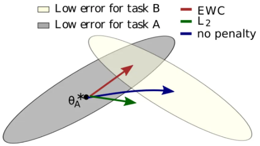
4.3 Principles behind the regularization by Elastic Weight Consolidation.. . . 41

4.4 Schematic representation of Progressive Networks approach (Fig. 1 from [RRD+16]). . 45

4.5 Restricted Boltzman Machine representation. Hidden layer h is densely connected to visible layer v by the weight matrix W. . . 52

4.6 Schematic representation of a GAN. . . 54

4.7 Schematic representation of the fearnet framework (Fig. 1 from [KK17]). . . 57

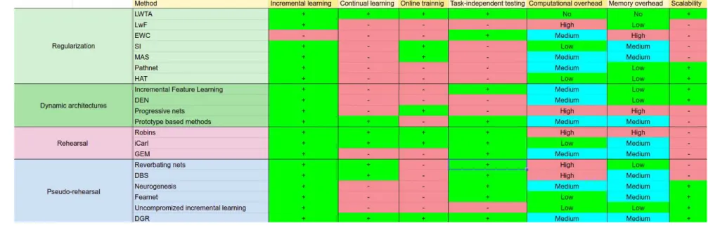
4.8 Comparison of existing methods aiming to alleviate catastrophic forgetting . . . 62

5.1 Simple synthetic 2D data. (Left) sampled data classes, described by 2D Gaussian distri-butions, (Right) input space partition by a NN classifier trained on the synthetic data from the left, white regions correspond to the uncertainty zones (cu=0.8) . . . 66

5.2 Space partition during sequential classifier training on class pairs. . . 67

5.4 Class-wise hidden layer activations when trained on full data, snapshot taken every 20

training epochs . . . 70

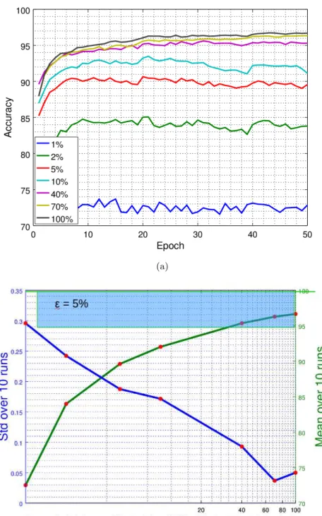
5.5 Results of the generalizability test on the MNIST dataset. (a) Classification accuracy

for different GANs support sizes as a function of training time. Average over 10 runs; (b) Mean/std of the classification accuracies for different GANs support sizes over 10 runs after 50 training epochs for the generalizability tests. Blue box represents the area

in which the generalization error does not exceed 5% . . . 73

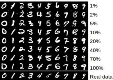
5.6 Samples, produced by DCGAN-based generator, when using 1 to 100% of the original

MNIST dataset to train it . . . 74

5.7 Representativity check of the DCGAN on MNIST dataset. This experiment

demon-strates the performance of the classifier trained on generated data, depending on the

amount of data sampled from the generator (% of the size of the original dataset). . . 75

5.8 Batch training accuracy on the original validation data for MNIST and LSUN dataset

when trained on real vs. generated data . . . 76

5.9 Schematic representation of our online learning approach. Original data is presented to

the model class by class. Each time new class of data appears we start training a new generator modeling that class. At the same time we train a classifier on the generated data from the previously learned classes and the original data from the new class that

come from the stream. . . 76

5.10 Adding a node to the output layer and initializing the connections with the previous

layer in the online learning scenario when new data class appears in the stream.. . . . 77

5.11 Stream classification scheme (for LSUN dataset, on MNIST no feature extraction is performed), described in this work. Stream is represented as an infinite sequence of

data intervals.. . . 78

5.12 Classification accuracy during online stream training for MNIST dataset . . . 80

5.13 Schematic representation of the way batches for the incremental learning are organized. N is the size of real data batch, coming from stream, n is the number of already learned

LIST OF FIGURES 7

5.14 Accuracy of the incremental learning on MNIST with different values of scaling

param-eter k for data regeneration . . . 82

5.15 Classification accuracy during online stream training for the LSUN dataset. Each point

on the graph corresponds to the average accuracy over 80 training intervals. . . 83

5.16 Average classification accuracy during stream training when the classifier is trained only on generated data. The curves correspond respectively to the average performance over all classes (gold), the average performance over classes pretrained before the beginning of the stream (red), and, the average performance over classes introduced during the

stream (blue) . . . 84

6.1 On the LSUN dataset, the effect of growing reconstruction error in autoencoders (leading

to catastrophic forgetting) when trained on their own reconstructions (blue line) and

the positive effect rehearsal has on this process (orange line). . . 99

6.2 Stream training on Syn-100. The results are shown for naive learning from stream

data (blue), learning with limited rehearsal (yellow), our method with the autoencoder trained with reconstruction loss only (green), with classification loss only (red) and full

method (purple). . . 100

6.3 Stream training on Syn-100. The results are shown for naive learning from stream

data (blue), learning with limited rehearsal (yellow), our method with the autoencoder trained with reconstruction loss only (green), with classification loss only (red) and full

method (purple). . . 100

6.4 Stream training on LSUN. The results are shown for naive learning from stream data

(blue), learning with limited rehearsal (yellow), our method with the autoencoder trained with reconstruction loss only (green), with classification loss only (red) and

List of Tables

6.1 The architectures of the classifier and autoencoder used in this study for the MNIST,

LSUN and Syn-1000 datasets. . . 94

6.2 Validation set accuracy on the pretrain part of the MNIST dataset, obtained during the

grid search aimed to optimize the trade-off between classification and reconstruction

losses in the autoencoders. . . 95

6.3 Validation set accuracy on the pretrain part of the LSUN dataset, obtained during the

grid search aimed to optimize the trade-off between classification and reconstruction

losses in the autoencoders. . . 96

6.4 Validation set accuracy on the pretrain part of the Syn-1000 dataset, obtained during

the grid search aimed to optimize the trade-off between classification and reconstruction

losses in the autoencoders. . . 96

6.5 Accuracies obtained on the validation sets of MNIST, LSUN and Syn-1000 depending

on the code size employed by autoencoders. The Base dimension is 784 for MNIST and

Part I

Chapter 1

Introduction

1.1

Motivation

In the last decades, computers and algorithms have become an essential part of our lives. In industries, they are used to increase productivity by thousands of times, thus saving billions of human working hours. They are actively employed in public and private services such as transportation and health-care, improving our daily routines and life quality. Moreover, computer-based technologies entered private life and changed the way people socialize, learn, and spend their free time.

This success is mainly due to the ability of modern computers to work with enormous amounts of data, efficient algorithms of data processing, and the growing capacity of computational systems. However, the most significant part of the solutions for real-life problems until recently was based on theoretical models and detailed algorithmization of the tasks developed and implemented by specialists in corresponding domains, engineers, and scientists. Such solutions suffer from several limitations: they are hard to design, require a considerable number of parameters to fine-tune, and are usually based on the human understanding of the phenomenon, which can be very approximate and imprecise. As a result, such methods are hard to generalize outside the task for which they are designed.

More importantly, when it comes to the problems considered “easy” by an average human, e.g., reading the hand-writings, detecting objects on the image, or recognizing a song from just the first few seconds of a recording, the direct algorithmization of the process is often extremely complicated. For instance, object detection, segmentation, and classification from natural images are intuitive tasks for humans.

However, one could hardly give step-by-step instructions for a computer to perform those tasks. This algorithmization complexity is the reason why the described tasks form a whole field of scientific research called Computer Vision. This domain has been studied for decades to achieve close to human performance in vision-related tasks.

In contrast to the approaches based on modeling and algorithmization, Machine Learning (ML) aims to make machines perform those tasks without giving explicit instructions. Instead, ML models extract knowledge directly from the raw data and corresponding annotations, if those are provided. Thus, the idea behind ML is to approximate a physical phenomenon by retrieving and organizing knowledge based on observations. Most of the ML methods store the knowledge in the parameters of the model. These parameters are optimized during the learning phase.

In contrast to a biological learning system that can continuously learn during its lifetime, most of the modern ML approaches learn in a static way from a predefined dataset of a limited size. In the era of robotics, social networks, and personalized gadgets that continuously collect user information, the demand for systems that can learn in real-time from vast amounts of data coming from multiple sources is rapidly growing. Due to this increasing need, the domain of online learning that aims to integrate new knowledge into the learning system in real-time has recently started to receive significant attention from the ML community.

1.2

Problem statement

The potential advantages of an online learning system over a system learning “in-place” from a pre-defined static dataset are numerous. The ability to learn continuously provides the learning system with the capacity to adapt to the changes in the environment and explore things never seen before. Besides, such a system should also be able to adapt to the evolving trends, tasks, updates in software and hardware, under the critical condition of not losing the previously acquired knowledge. The ap-plications of an online learning system can vary from predicting the hash-tags of the images taking into account the latest trends to creating the humanoid bots, which can adapt to the rich and rapidly changing real-world environment.

1.2 Problem statement 15

Compared to training on static data, online learning from the streams introduces several new relatively unstudied challenges. First of all, data streams can suffer from drifts in the underlying distribution due to the changes in the emitting environment, sensors used to retrieve the data can be replaced or updated, or the task of interest can change over time. In such conditions, models tend to fit the distribution of currently available data, which may result in drastic changes in the inference mechanism. Moreover, online learning systems have to learn from the continuously arriving data, which means that the learning mechanism should be able to retrieve all the necessary information in real-time.

To summarize the challenges mentioned above and formalize the requirements one should impose on the online learning system, let us state that such a system should be provided with the following characteristics:

1. Real-time data processing.

2. Fast knowledge incorporation from limited data. 3. Mechanism to protect already acquired knowledge. 4. Efficiency on data of a very high complexity.

5. Scalability to large problems with a significant number of classes.

One can obtain most of the described characteristics by imposing certain conditions on the training procedure (1), the model’s design (5), or even the type of the model employed (4). In contrast, (2) and (3) are challenging to handle and often interfere with each other. The literature dedicated to learning in biological and computational systems often addresses the relation between the ability of the system to incorporate new knowledge (2) and retain the old one (3) as the stability-plasticity dilemma ([Gro82], [MBB13]). This notion, while not frequently mentioned in the rest of the thesis, is the core problem of our study.

More specifically, in this thesis we focus on the problem of online image classification in a continuous stream context. While useful in a large number of practical computer vision applications, image classification is an acknowledged difficult problem, largely still unsolved in the general case. Moreover, image classifiers need large training sets to perform reasonably well, while dealing with image databases

is very resource-intensive both in terms of storage and computing power. These conditions make it very challenging to perform online training on streams of image data, moreover so because the incoming data is heavy and difficult to store, while the task to solve is complex and requires updating large learning models.

Until recently, the most widely used methods for classification on data streams included Hoeffding trees ([DH00]), Bayesian trees ([SAK+09]), Support Vector Machines ([RDIV09]) and ensemble methods

([Oza05]). A comparative overview of these methods is presented in ([NWN15]). The conclusion is

that, even though they allow real-time testing, can efficiently handle concept drift ([WHC+16]) and do not face memory issues, those methods do not perform well on complex high-dimensional data, thus not satisfying (4).

In comparison, methods based on Deep Learning (DL) are efficiently handling complex classification tasks on high-dimensional data with up to a few thousand classes. In recent years, DL-based ap-proaches have become state of the art in numerous applications, such as image and signal classification

([KSH12]), object detection ([SKCL13]) and segmentation ([HGDG17]), natural language processing

([SVL14]), ([CWB+11]) and many others. Despite its popularity and efficiency on high-dimensional

data of significant structural complexity, most of the currently existing deep learning approaches are aiming to solve offline learning problems where all the data are constantly available during training. Training DL models on non-stationary stream data with a changing distribution of data classes gener-ally leads to a phenomenon of catastrophic forgetting ([MC89]). The knowledge encoded in the neural connections is gradually overwritten by new information in the absence of data reinforcing previous knowledge, i.e., data corresponding to previously learned classes or to different modes of the current classes.

Currently existing solutions to overcome catastrophic forgetting in Neural Networks include three types of approaches: methods based on training regularization where the network updates depend on the importance of the neural connections for the historical tasks; networks with evolving architectures, able to grow and adapt to the increasing complexity of the problem; and the approaches that make use of a supplementary memory unit that provides the model with missing data classes. In Chapter4,

1.3 Conventions and notations 17

we discuss in detail the existing methods from each of the three groups. This bibliographic chapter shows the reader the reasoning behind our choice of direction for the study.

1.3

Conventions and notations

In this section, we introduce several notions and conventions that hold for the rest of the manuscript. We do so to facilitate the understanding of the proposed methodology, avoid confusion in terminology, and provide the reader with a brief overview of the experimental scenarios on which we validate our approaches.

Dataset and data stream. We discriminate between the notions of the dataset as a predefined static collection of data samples, and the data stream (sometimes referred to as data source) as a process of continuous retrieval of data samples from the changing environment. The essential difference between the two is that in the case of the dataset, one can manipulate the collection of data prior to learning, e.g., balance data classes, perform several steps of pre-processing, study the data statistics, etc. All this becomes hardly conceivable when working with data streams.

Learning system. In our study, we employ sophisticated systems that contain several learning blocks, each having its own learning rules, structure, and schedules. For the sake of simplicity of appealing to the full learning mechanism, we call the complete set of architectures used to perform learning for a given problem as a learning system.

Learning tasks. In most cases, the term task is used in a global context referring to the objective of learning (e.g., classification task, generative task). This notion, however, is sometimes employed to describe a sequence of sub-problems of the global learning problem. To make it more clear, let us consider an example of classification on a dataset containing N separate classes. In these settings, we can imagine a situation in which only a subset of all the different classes is available at each time interval. Thus, we can describe learning on each of these intervals as a separate task.

Online learning This term is used to describe in a very general manner any learning process that involves incorporating knowledge from data streams.

1.4

Contributions of the thesis

As mentioned before, one of the biggest challenges in deep online classification training is to avoid forgetting the already acquired knowledge. A straightforward solution to this problem is rehearsal

([Rob95]) that consists in storing all (or at least a significant part of) the historical data together with

newly arriving stream data and retraining the classifier on all the available information every time the model has to be updated. However, if the system is required to learn on high-speed data streams and keep acquiring new knowledge for an extended period, or has to perform life-long learning, such an approach fails to scale to the size of the problem. To avoid the difficulties related to historical data storage, we take the line of research that focuses on using generative models to approximate the statistical distribution of the source ([PKP+18,SLKK17,KGL17]).

In the first contribution of this work (Chapter5), we address the incremental classification problem, where classes appear in the stream one by one, and a particular type of continuous stream with several classes being available at each time interval. In the proposed approach, we employ Deep convolutional Generative Adversarial Networks (DCGANs [RMC15]) to make up for the absent data classes. We initialize a separate DCGAN for each newly appearing class. We then train them during the stream phase when corresponding data are available to produce images that are visually close to the input source. Each time a data class disappears from the input stream, we use the previously learned GANs to generate new samples for the missing categories. This procedure allows us to ensure that all classes (past and present) are equally balanced in the current learning batch. The proposed approaches for incremental and continuous cases resulted in papers [BBCF17] and [BBCF18] correspondingly. While this approach has merits and works reasonably well on many databases, the use of GANs has some drawbacks. First, the quality of the generated samples is very class-dependent as the internal structure of the objects influences the learning process. Second, training GANs is an unstable process, especially for data of high complexity. It may affect the quality of the generated samples when new

1.4 Contributions of the thesis 19

real examples of a class arrive. Finally, GANs are extremely slow to train. In the incremental learning settings where one can learn each new class until convergence, slow training is not an issue. However, such behavior makes the proposed approach fail to scale to more complex scenarios where real-time training is required.

The second contribution of the thesis (Chapter6) presents a more general approach that can work with more complex continuous data streams with no specific order in class appearance and is scalable to a much larger pool of available classes. The proposed learning framework uses auto-encoders for long-term memory purposes to overpass the previously described limitations of GANs. The auto-encoders are significantly faster to train than GANs. At the same time, using auto-auto-encoders allows us to train a single model to learn all the historical classes. This significantly reduces the memory requirement of the learning system. To further improve the performance of the proposed approach, we enhance the auto-encoders training procedure by adding a supplementary loss function that measures the classifier’s performance on produced samples. Moreover, to avoid the drift in the distribution of samples reconstructed by the auto-encoders when the latter is trained on its own reconstructions, we propose a technique of adaptive gradient weighting. This method modifies the influence of the synthetic samples depending on the number of full encoding-decoding passes they went through. We validate the proposed method on the continuous streams simulated from static natural image datasets and a large-scale synthetic dataset designed for this study. We demonstrate that the proposed approach is fast, scalable to large problems with thousands of classes, and has a stable training process. The described work was submitted to the Computer Vision and Image Understanding journal. The rest of the thesis is organized as follows. In Chapter2, we describe the theoretical background of online learning and give detailed information about the experimental scenarios we address. Chapter3

provides a brief discussion on the DL principles. We explain how the standard learning procedure in Neural Networks leads to catastrophic forgetting. In Chapter 4, we review existing methods that address the problem of online learning on data streams and position our proposals with respect to these. We give a detailed presentation of the most relevant proposals in three types of methods for online learning: dynamic architectures, regularization, and dual-memory based approaches, and

highlight their main advantages and limitations. In Chapter5, we describe our first proposal that uses GANs to preserve and replay historical knowledge. We demonstrate that the proposed method can efficiently perform incremental learning by validating it on two image datasets simulated as incremental data streams. In Chapter 6, we present our second approach, able to perform continual learning on dynamic data streams using auto-encoders. We discuss the advantages of auto-encoders over GANs to replace historical data in such an advanced scenario. We describe our learning framework, assess its performance by an experimental validation on three different datasets, and analyze its behavior. Finally, in Chapter7, we discuss perspectives and future work.

Chapter 2

Learning from Data Streams

The goal of this thesis is to develop approaches that can learn in a fast and efficient way from data streams with dynamically changing data distributions and multiple factors that can influence training in real-time. To develop such a method, we first need to give a more formal definition of the problem and discuss its currently existing solutions.

In this chapter, we formalize the context of continual learning from data streams. We start by intro-ducing the main definitions of the domain and discussing the challenges that one faces when dealing with it, notably the issues related to the phenomenon of the concept drift. We then discuss different types of learning scenarios that fall into the domain of online learning.

2.1

Online learning

Online learning has only recently received serious attention from the ML community. The field is therefore not well established yet, missing agreement in definitions and baselines. As an example, the following recent works [HKCK18], [KMA+17], [LP+17] and [MCH+18] all deal with online learning. A quick look at the learning scenarios and definitions proposed in these papers is enough to see that different authors try to solve relatively different problems. In this section, we propose our definitions of the discussed concepts. These definitions differ, to some extent, from what the reader may find in the literature. However, for the sake of clarity, we hold on to proposed notions for the rest of the thesis.

Let us first introduce the notion of the learning environment as the surroundings and conditions in which a learning agent lives or operates. As previously stated, in this work, we mostly deal with supervised learning. Let us, therefore, consider that each environment is partially or entirely annotated by human experts.

Let us introduce a group of agents (ai)|_iA=1 dynamically exploring a potentially infinite set of

envi-ronments (_Ej)∞j=1. Each agent ai is provided with a set of sensors (c(_kai))|C_k=1 that capture specific

representations from the environment (e.g., images, sounds, other sensory information). We denote these representations as data samples

s={~x1, . . . ,~xk, . . . ,~xC} = {c(_ka)(E)}Ck=1

where each data feature~_{xk is a specific numerical representation of the environment acquired by the}

kth sensor of an agent. In the supervised learning context, one or several features provided by the agent have to correspond to environment annotations (training targets). To keep the notations simple and homogeneous, we put the target value (or values) in the last positions of the data sample in the following way:

s=_{~x1, . . . ,~xk, . . . ,~xC,~y}

We denote_{E =}S∞

j=1Ej the complete environment available for the agent population. To link the data

and the environment, let us say that data are the perception of the environment by the learning agents. We then assume that the data acquisition procedure is discrete and that data samples can be rapidly transferred to a centralized learner L with no time overlap between separate transfers. This assumption allows us to introduce the following definition of a Data Stream..

Def. We call Data Stream the following agent–learner communication procedure:

S = [st=c ai(t)

k(t)(Ej(t))]t|∞t=0

where st is a data sample acquired from the environment Ej by the sensor ck of the agent ai and

2.1 Online learning 23

In real-life applications, a data stream in the provided formulation certainly has one or several proper-ties that make real-time learning very challenging. First of all, depending on the application, data can arrive extremely fast. Second, in contrast to learning from static data, when learning from streams, there is no guarantee that data classes are balanced and that the system does not suffer from dramatic drifts in the underlying data distribution. However, even in the presence of distribution changes and incrementally appearing classes, different data categories can still share internal representations and have temporal dependencies that may be extremely useful for the fast incorporation of new knowledge. Therefore, an efficient online learning system should be provided with the following characteristics:

1. Learn fast from few examples and from unequally represented concepts.

2. Continuously learn for long periods of time on long data sequences, potentially for the life duration (life-long learning).

3. Detect and handle drifts in data distribution and adapt to different types of data.

4. Efficiently use previously acquired knowledge when learning new tasks (knowledge transfer). 5. Adapt to new data concepts never seen before, with the total number of categories unknown in

advance and potentially very large.

6. Long-term memory capacities – ability not to forget already acquired knowledge.

To be able to generalize from the training set to the test set, one needs to assume that there is some common structure in the data. The most commonly used set of assumptions are the i.i.d. assumptions. They state that the data is independently and identically distributed: each example is generated independently from the other examples, and each example is drawn from the same distribution Pdata.

The property of unequally distributed data classes in a given batch of the stream and dynamically changing data concepts is often addressed in the literature ([HKCK18], [LP+17], etc.) as the non-i.i.d. nature of the data in the stream. This implies that the batches (1) are not randomly sampled from the training data (streaming data may have temporal/spatial dependencies due to the continuity of the observed environment) and (2) are sampled from a changing distribution (not identically distributed).

Depending on the type of the stream and the tasks the model has to solve, online learning can be divided into several sub-domains.

Incremental learning is the sub-case of continual learning in which a single agent explores envi-ronments one by one, with each environment being locally i.i.d. In the most frequent case, this type of learning consists of introducing new objects to be explored by the system. Such a problem formulation can find its utility in real-life applications where data arrive in a very specific and well-organized order.

Transfer learning is another type of learning which aims to transfer knowledge from one task to another. The transfer learning paradigm usually does not require retaining previously acquired knowl-edge but instead aims to use this knowlknowl-edge to accelerate and stabilize the procedure of incorporating the information from the current task.

In this thesis, we do not claim any contribution to the domain of transfer learning. However, we use some transfer learning techniques, such as feature extraction by pre-trained models. We employ them as auxiliary tools to facilitate our experiments.

Continual learning is the learning paradigm that is of the main interest to this thesis. Similarly to incremental learning, data are continuously arriving at the learning system and have to be rapidly processed. However, in continual learning, we do not make any assumption about the proper separation between the tasks and the availability of task descriptors at training time – instead, we consider the full learning procedure as a single task that evolves with time.

Remark on centralized learning. The requirement for centralized learning, mentioned earlier in this section, may produce security and privacy concerns for various applications where only in-place training is allowed. However, we argue that this condition is of high importance in designing a comprehensive life-long learning system. However, one can easily project the proposed definitions onto the case of a pre-trained system that has to be locally fine-tuned. To do so, one can provide a single agent with a pre-trained learner, updated exclusively on locally available data. Such a system

2.2 Concept drift 25

usually has to fit a specific application in a limited environment; therefore, learning is relaxed on several requirements that we impose in the case of life-long learning. We, therefore, assume that this scenario is of no particular interest to this thesis.

2.2

Concept drift

In most real-life applications, data distribution is changing over time. This phenomenon is usually referred in the literature as concept drift. The notion of concept drift describes the characteristics of a data stream. In this section, based on the review papers ([WHC+16], [GˇZB+14]), we provide a brief overview of the existing ways to detect and handle concept drifts in data streams. We believe that this introduction can help the reader better understand the type of data and the complexity of the task we aim to solve in this thesis.

Multiple factors can cause changes in the data distribution. To demonstrate it, let us consider the following scenarios:

1. A learning agent is pre-trained on a base environment containing data classes 1, . . . , n, and is sent in its original configuration, with no modifications in its receptors and data pre-processing mechanisms, to explore new environments and learn new classes n+1, . . . , n+m.

2. The same learning agent, instead of being sent out, is kept training on the base environment, but the learning conditions are changed, e.g. it is now learning from the images captured by different sensors, in a much lower level of light (night mode) or in the presence of other artifacts that introduce noise.

3. The data environment stays exactly the same, but the learning task is changed, e.g. the original task of detecting and classifying animals on a farm switches to distinguishing between indoor and outdoor images.

All three described situations can be challenging to handle by a learning system. To understand the potential difficulties one can have when dealing with those situations, let us formalize the problem. Let us consider a scenario of supervised learning from the stream (see Sec. 2.1), where the learning

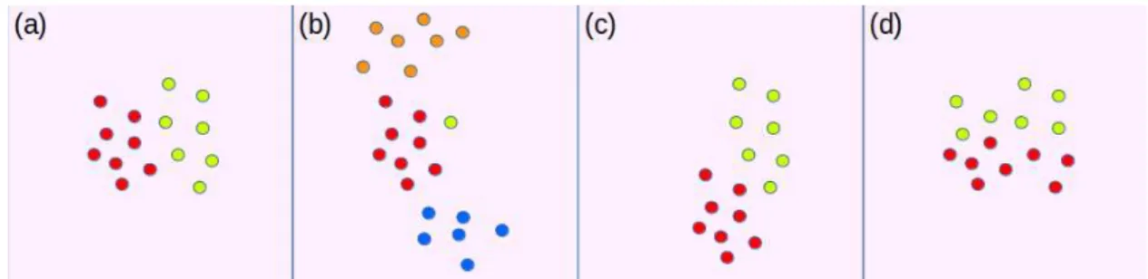
Figure 2.1: Representation of different possible changes in data distribution. (a) Initial distribution with two classes; (b) p(y)is changed, the green class almost disappeared, two new classes are added; (c) changes in p(X|y) (virtual concept drift); (d) data set stays the same, but the label distribution p(y|X)changes (real concept drift)

system continuously receives data samples s= (Xt, yt) from the environment. We also consider that

data emitted by the source at time t follow the joint input-output distribution pt(X, y). We then say

that the data stream suffered from concept drift in the time period[t0, t1]if

pt0(X, y)6=pt1(X, y)

With these notations, the previously discussed situations can be seen as follows (see Fig. 2.1 for an illustration):

1. Changes in the prior probabilities p(y)(Fig. 2.1 [b]).

2. Changes in class conditional probabilities p(X|y)– virtual concept drift (Fig.2.1 [c]). 3. Changes in posterior probabilities p(y|X)– real concept drift (Fig.2.1 [d]).

In standard learning paradigms often discussed in the DL literature, dealing with the first two types of drift can be seen as improving the generalization capacities of the learning model. Indeed, in both cases, the drifts in data distribution are most probably temporal, with many possible variations of those changes. Therefore the main objective of learning on such a stream is to create a general model able to perform its main task independently from the changes in the data distribution. One of the most significant issues that can arise when dealing with such drifts is catastrophic forgetting – the core problem this thesis is addressing, that is discussed in detail in the next sections. In contrast, real

2.2 Concept drift 27

to a relatively new task in the fastest and most efficient way – a problem often referred to as transfer learning.

From the other point of view, drifts in prior probabilities p(y) mostly represent the global changes in the modeled phenomenon rather than changes in the data distribution. Therefore, only the types of data evolution described at points (2) and (3) are usually considered concept drift.

To deal with the previously described changes in streaming data distribution, a learning system must be able to detect concept drift as soon as possible, distinguish it from noise and adapt to it. Besides, one of the main ideas of online learning is that the most recent data should be the most relevant to the model of interest. Therefore the efficient concept drift handling mechanism should not only be able to incorporate new knowledge, but also remove the out-of-date information. Depending on the desired result, one can choose a forgetting method with an adequate trade-off between its reactivity and robustness to noise. Ideally, the system is forced to forget already trained parts of the model if and only if it detects a drift in data distribution with certainty that this drift is not due to noise. A very intuitive solution to adapt to changes in data distribution is to introduce a memory term to the online learning model. It can be done by adding a sliding window that tells how many most recent data samples one can store in our model and use to verify if the data distribution has recently changed. There exist many methods to detect concept drifts in data. Generally, these methods characterize and quantify changes in the data distribution at a given time point or during some time interval and can be based on: 1) sequential analysis, 2) control charts, 3) differences between two distributions and 4) heuristics.

Detectors based on sequential analysis. The Sequential Probability Ratio Test (SPRT) is based on detecting the potential changes in data distribution at time point w : t0≤w≤t1 by computing

the ratio between the probabilities of the data sub-sequence, arriving after w, to come from P1=Pt1

rather than P0=Pt0.

Tnw

=

=

We say that the change at time point w is detected if Tnw is above a user-defined threshold. Methods

Detectors based on Statistical Process Control. Let us consider a sequence of examples(Xi, yi).

For each data sample Xi our classification model predicts ˆyi which is either true ( ˆyi =yi) or false

( ˆyi6=yi). For each example we define the probability pi of detecting a wrong label with the standard

deviation σi=p pi(1−pi)/i. We also define two parameters pmin and σmin that are updated if, for a

given sample pi, pi+σi<pmin+sigmamin.

For a newly arriving data sample (Xj, yj) with pj and σj defined by the current model, we say that

the sample is in-control if pj+σj <pmin+2σmin, out-of-control if pj+σj >pmin+3σmin and in

warning state otherwise.

With enough data, we can use Out-of-Control examples as Concept drift detectors. One more useful measure that can be defined based on obtained information is the rate of change – the time it takes to pass from Warning to Out-of-Control.

Monitoring distributions on two different time windows. Methods from this group usually consist of fixing windows on the historical data and new arriving data and introducing a statistical test that has a hypothesis that distributions in two windows are equal. If the hypothesis is rejected, then data drift is declared.

Methods can vary from more reactive to more stable depending on the window size. The main limitation of these approaches is that we have to store the data from the chosen windows. The advantage is usually a much more precise localization of the change point compared to sequential methods.

2.3

Experimental scenarios for online learning

In previous sections, we presented the theoretical background of online learning. However, this theory is not straightforward to apply to real problems. First of all, real massive data streams are very difficult to obtain, process, and especially make reproducible studies on them due to the dynamic nature of the data. To overcome this, the validation of the methods for online learning is usually performed by casting the data from classic static datasets in the form of streams. In this section, we review several existing setups of the experimental validation of online learning, notably the cases proposed in [GMX+13].

The authors of [GMX+13] propose to evaluate forgetting when learning from a sequence of tasks. While in the original paper, the authors only perform experiments on two tasks, we extend the described framework to the series of K distinct tasks. Let us consider a sequence T={T1, . . . , Tt, . . . , TK} of K

tasks, each provided with a corresponding dataset Dt={Xit, Yit}i=1...Nt, where Nt is the size of the

corresponding dataset. The goal of each task is to optimize the parameters θ of the model C that learns to map each input X to the corresponding output Y by minimizing the task-specific loss function Lt(Cθ(X), Y). The global objective of this multi-task learning is to minimize the loss over the full set

of tasks: min θ K

∑

2.3 Experimental scenarios for online learning 29

While the described framework is very general and can be adapted to any task sequence, in the discussed work, the authors consider three different types of tasks that allow studying model behavior under different angles.

Input reformatting: permutation tasks. Training dataset D=_{Xi, Yi}is the same across all the

tasks. For each new task, the input data distribution is changed by applying a task-specific transform Ft while corresponding outputs stay unchanged so that for each task Tt its corresponding dataset can

be described as Dt={Tt(Xi), Yi}i=1...K. As an example of such a transform, the authors propose to

apply a fixed pixels permutation on the input data for each new task. Such a scenario can be naturally related with the applications prone to the virtual concept drifts (see Chapter2.2).

Similar tasks. Similarly to the previously described tasks, here, the input-output domains are similar – the tasks differ from one another by a slight drift in the data distribution. As an example, the authors perform their validation on two product categories in the Amazon reviews dataset ([BDP07]) with the binary sentiment analysis as the primary learning objective.

Dissimilar tasks. Data for each new task are coming from a different distribution, for instance, from a completely different dataset. Learning in this way is natural for humans, who can learn from various sensory inputs in different environments and successfully transfer knowledge across different domains of expertise. To the best of our knowledge, there exists no artificial learning system that proved its capacities of efficient knowledge transfer across entirely dissimilar tasks where the inputs don’t share any common characteristics. In the current state of the art, the described problem is referred to as Artificial General Intelligence. It is mostly approached by incrementally adding new modules to the model, each solving a new task, with almost no positive knowledge transfer between the modules. From this point of view, existing approaches do not differ from training one model per task and do not represent any particular interest for our study.

Online classification task. In this study, we address the problem of online learning for data clas-sification. In accordance to the notations introduced in Sec.2.1, we can formalize the global objective as learning from a long sequence of tasks, where each task corresponds to training in the environment Ej which is a part of the global environment E containing only a limited number of data classes. In a

real-life application with a large population of agents, each task would correspond to a separate time interval during which only a specific group of agents are actively learning, or only a small part of the global environment is explored.

Chapter 3

Deep learning background

As we have already mentioned in the introduction, there exist several types of non-DL methods that proved their ability to perform online learning. These methods are, however, not efficient when applied to streams of high-dimensional data (e.g., natural images), which brings us to the necessity to build our learning system based on Neural Networks.

The main technical challenge that we address in this thesis is catastrophic forgetting in NNs. However, going into a more in-depth discussion of this phenomenon, it is crucial to understand its nature and origins. We argue that this is only possible with a fundamental understanding of the Deep Learning machinery. Basic Deep Learning concepts are not the primary objective of this study. However, in this chapter, we provide a brief introduction to the DL background, which helps us to understand the difficulty of training Neural Networks on dynamic data and to get the first idea on how to approach the problem.

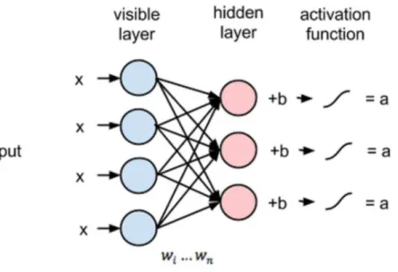
Neural networks, the core model of Deep Learning, are originally designed to reproduce in a very simplified way the biological brain functioning. The formal objective of such models is to approximate a function that maps some input vector to the desired output, corresponding to this input. The term “Deep Learning” is related to the deep multi-layer structure of these networks. Each layer is a composition of a simple affine transformation of the output of the previous layer and of a non-linearity. In theory, such a structure is supposed to allow the network to approximate any function of interest. The output layer of the network represents the space of desired outputs, which depends on the application – the actual function the network has to approximate. It can be represented by a single value for the case of binary classification and fault detection, by a vector of probabilities for multi-class classification, or lie in the input space when we want to build a model that recovers corrupted data (autoencoders) or to perform some modification or processing on the input.

3.1

Inference in Neural Networks

Neural Networks in their standard formulation are models built from a sequence of linear layers (affine mappings), each followed by an activation function (a non-linearity). More formally, denoting the

input vector by X, linear layers by li and activation functions by σi, an n-layers Neural network can

be represented as a composition of functions in the following way:

y∗=l0◦σ0◦l1◦σ1◦ · · · ◦ln(X)

Linear layers in these notations are simply the following matrix operation: l(X) =WX+b, where the matrix W is usually called neural weights, and b is the vector of bias. Weights and biases form the parameter space of the model. In recent applications where extremely deep models are used on complex high dimensional data, this space can reach the dimension of several billions of parameters. The activation function, in turn, can be any almost everywhere differentiable non-linear function defined over the vector space. However, for reasons like numerical stability and empirically proved effectiveness, most of the currently employed DL models use the following activation functions:

• Sigmoid function: σ(x) = 1 1+e−x

• Tanh function: σ(x) = 2 1+e−2x −1

• Rectified Linear Activation (ReLU): σ(x) =max(0, x)

3.2

Backpropagation: principles behind NN optimization

As it was previously said, Neural Networks are models having as parameters neural weights W and bias terms b. To simplify the further notations, let us group the neural weights and the bias terms in the single parameter set W. To approximate a function, one needs to find the values of those parameters that map the inputs of the network (X) as close as possible to the desired output (y). The very first step is to define the objective (or loss) function that computes the proximity of the actual output of the network (y∗) and the desired one. The goal of optimization in Deep Learning is to search for a set of parameters W∗ that minimizes the loss of the network over the available training data samples:

W∗=argmin_W∈Rn

∑

where J is a loss function that evaluates how far the real output is from the desired one.

There exist various approaches to optimize parametric models. The most widely used methods for Neural Networks are derived from the simple Gradient Descent:

Wi+1=Wi− α

N_x∈X,y

∑

where N is the number of samples in the training set and α is the learning rate. Computing the gradient of high dimensional parametric models is, however, not an easy task.

The most straightforward way to evaluate the gradient of the cost function with respect to the net-work parameters is to compute its numerical estimation by adding tiny variations separately for each

3.3 Optimization in Neural Networks 33

parameter wi of the network and verifying how much it influences the output:

dC dwi

= C(wi+ǫ)−C(wi)

ǫ

This method was widely used in the early ages of NN history. However, to perform a single update, such methods require propagating information through the big part of the network for as many times as there are parameters, which is extremely slow and becomes almost unfeasible even for problems that are nowadays considered small and simple.

A more efficient way to compute gradients, that became the gold standard in Neural Network optimiza-tion, is gradient backpropagation ([WH86]). The method is an application of the classic differentiation “chain rule” and consists of an analytic computation of the derivative of the objective function over each layer of the network. As it was already mentioned, all the layers of Neural Networks are almost everywhere differentiable. Moreover, the widely used types of layers are designed in such a way that each layer i of the network can be easily derived over the layer i−1 with the analytic derivative represented by either a matrix multiplication or, in the case of activation layers, by the element-wise vector operations. In this way, once the loss function is used to compute the error of the network on a given input-output pair, this error can be “back-propagated” through the full network in a single pass, thus estimating the gradient of the loss over the full set of parameters.

3.3

Optimization in Neural Networks

In the previous section, we discussed the mechanism of gradient descent applied to NN optimization. However, we only mentioned how the optimization is supposed to work to correctly map a given sample. Deep learning problems usually consist of optimizing the model to learn huge datasets of up to thousands of different classes, each represented by millions of data samples. The global objective, in this case, is usually to approximate a function that produces the smallest possible error on the available training data, rather than just fitting a given data sample. Ideally, one could first compute the error on the totality of the available training data and only then back-propagate it and update the parameters. However, such a procedure is extremely slow.

On the other hand, one can try to compute the error and update the network sequentially on each separate data sample. This way of performing optimization is known to have a very low generalization. Due to the high-dimensional parametrization of Neural Networks, consecutive data samples can have very distant local minima provoking high oscillations in the computed loss and thus resulting in gradient descent divergence.

It was empirically demonstrated that what works best is performing the parameter updates on mini-batches of randomly selected data samples. Indeed, such a procedure averages the error over a small batch of data samples, potentially significantly different. This provides a better approximation of the direction of global minima and smooths the optimization trajectory.

the gradient descent with an additional term – the momentum ([SMDH13]). In this case, the network parameters are updated in the following way:

vt+1=µvt−ǫ∇f(θt)

θt+1=θt+vt+1,

where θt are the model parameters at step t, µ and ǫ are the training hyper-parameters, usually called

momentum coefficient and learning rate. As can be seen from the formula, the momentum term is accounting for the recent history of parameter updates, thus, to some extent protecting the gradient from dramatically changing directions. The idea of smoothing the gradient by accounting for its history was pushed even further in the method called Adam ([KB14]), which also adapts the learning rate separately for each layer of the network. Due to its numerical stability and fast convergence, Adam is nowadays one of the most widely employed optimization techniques. We, therefore, decided to use it in our experiments.

3.4

Importance of the initialization in neural networks

Until recently, Neural Network parameters were often randomly initialized from the normal distribu-tion. Due to the often occurring divergence during the early training stages, very deep NNs initialized in this way were considered extremely difficult to train until [HOT06] proposed to initialize deep net-works from pre-trained blocks. While this technique slightly improved the situation, training in such a way required significant computational resources and still had stability issues.

The problems mentioned above are often characterized by the exploding or vanishing values in the activations of the network. The reason for that is the nature of the basic operations of the neural networks – matrix multiplications. For the simplicity of demonstration, let us for now consider neural networks with no activation functions and no bias terms. In this case, each activation a(_jl) of a layer l of the neural network is a weighted sum of the activations from the previous layer:

a(_jl)=

N(l−1)

∑

i=1

w_ij(l)a(_il−1)

Assuming that both weights and input data (x=a(0)) have zero mean (normalizing data to have zero mean is a standard procedure), the expected value of the activations at all the layers will also be zero:

E[a(_jl)] =N(l−1)E[w(_ijl)]E[a(_il−1)] =0

The variance of the activations, in this case, depends on the distribution of network parameters, input activations and, importantly, on the size of the previous layer:

3.5 Generalizing to unseen data 35 Var(a(_jl)) = E[( N(l−1)

∑

∑

Therefore, if all the parameters of the network are initialized from the normal distribution (Var(w(l)_{) =}

1), then the standard deviation of the activation will be scaled by√N(l−1)_{at each new layer which will}

rapidly result in exploding activation values. Initializing the weights with lower variance can result in a completely inverse “vanishing” effect with the network activations having a lower deviation from one layer to the next. At the same time, when performing the backpropagation, the variance of the gradient of the parameters between layers l−1 and l depends on the size of the layer l instead of l−1, as it was for the forward pass. It is therefore clear that one should initialize the weights separately for each layer with the variation that depends on the sizes of the layers l₋1 and l.

While the mechanism inevitably changes when one adds the non-linear activation functions at each layer, the previous logic holds. However, in addition to the layer size dependency, one now also has to adapt the initialization to the type of activation functions. In [GB10] the authors propose the Xavier initialization method that takes into account all the discussed points for the case of hyperbolic tangent and softsign activation functions:

W(l)∼U " − √ 6 p N(l−1)_+N(l), √ 6 p N(l−1)_+N(l) #

To train the networks with ReLU activations, the authors of [HZRS15] propose the following Kaiming initialization:

W(l)∼ N (0, 1)·

r 2 N(l−1)

According to the mathematical evidence presented in the paper, in the case of ReLU activation function initialization requires only one parameter of the layer size (input or output of the layer) to ensure stable training with no value explosion.

3.5

Generalizing to unseen data

Over-fitting is a significant problem in ML in general, and in DL in particular. It naturally arises from the way learning is performed. The NN’s optimization fits the data in the training set, aiming to build the precise input-output mappings. In the static learning case, the problem usually comes from the extremely high dimension and variability of the input data. Indeed, Neural Networks can be seen as the statistical approximations of the input data. When the data are high dimensional