Botanical Computing: A Developmental Approach to
Generating Interconnect Topologies on an Amorphous
Computer
by
Daniel N. Coore
SB, Massachusetts Institute of Technology, 1994
SM, Massachusetts Institute of Technology, 1994
Submitted to the Department of Electrical Engineering and Computer Science
in partial fulfillment of the requirements for the degree of
Doctor of Philosophy
at the
MASSACHUSETTS INSTITUTE OF TECHNOLOGY
February 1999
@
Massachusetts Institute of Technology 1999. All rights reserved.
Author ... ...
Department of Electrical Engineering and Computer Science
January 28, 1999
Certified by....
Gerald J. Sussman
Matsus ita Professor of Electrical Engineering, MIT
^ Thesis Supervisor
Certified by... . . ... ... ...
Harold Abelson
Class of 1922 Professor of Computer Science and Engineering, MIT
Thesis Supervisor
Accepted by...
...
...
Arthur C. Smith
Chairman. Deoartmental-Qaddittee on Graduate Students
Botanical Computing: A Developmental Approach to Generating
Interconnect Topologies on an Amorphous Computer
by
Daniel N. Coore
Submitted to the Department of Electrical Engineering and Computer Science on January 28, 1999, in partial fulfillment of the
requirements for the degree of Doctor of Philosophy
Abstract
An amorphous computing medium is a system of irregularly placed, asynchronous, locally interacting computing elements. I have demonstrated that amorphous media can be con-figured by a program, common to all computing elements, to generate highly complex prespecified patterns. For example, I can specify that an amorphous medium manifest a pattern representing the interconnection structure of an arbitrary electrical circuit.
My strategy is inspired by a botanical metaphor based on growing points and tropisms.
To make this strategy explicit, I have developed the Growing Point Language (GPL). A growing point is a locus of activity in an amorphous medium. A growing point propagates through the medium by transferring its activity from one computing element to a neighbor. As a growing point passes through the medium it effects the differentiation of the behaviors of the computing elements it visits. The trajectory of the growing point is controlled
by signals that are automatically carried through the medium from other differentiated
elements. Such a response is called a tropism. In this way a GPL program can exploit locality to make crude geometric inferences.
There is a wide variety of patterns that are expressible in GPL. Examples include: Euclidean constructions, branching structures and simple text. I prove that amorphous media can be programmed to draw any prespecified planar graph, and I obtain upper bounds on the amount of storage required by the individual processors to realize such a graph. I also analyze how the effectiveness of GPL programs depends upon the distribution of the computing elements.
Thesis Supervisor: Gerald J. Sussman
Title: Matsushita Professor of Electrical Engineering, MIT Thesis Supervisor: Harold Abelson
Title: Class of 1922 Professor of Computer Science and Engineering, MIT Thesis Reader: Thomas F. Knight
Acknowledgments
1There are a number of people to whom I am indebted for their support and encouragement. Kanchi, my wife and strongest supporter, who proofread my drafts, discussed my in-choate ideas with me and helped me to develop them, and generally kept me on track over the past year.
Gerry Sussman for issuing the challenge in the first place, for providing plenty of nurtur-ing guidance and energetic encouragement along the way. Hal Abelson for the many useful comments and keen advice on how to improve the dissertation.
Tom Knight for the useful and encouraging comments at the beginning of the project. Jacob Katzenelson for carefully reading the proposal as well as the dissertation and ask-ing generally good questions. Those questions forced me to address many issues I might otherwise have overlooked.
Radhika Nagpal, Ron Weiss, Erik Rauch, Jeremy Zucker, Piotr Mitros, Chris Laas and the rest of Swiss group for providing helpful input at various times throughout the whole endeavour.
Rajeev Surati, Elmer Hung and Natalya Cohen for offering playful competition and supportive encouragement along the way.
Hoang 'ran, Nyssim Lefford and Frank Cortez, my supportive apartment mates, who would offer to feed me (when Kanchi wasn't around) whenever it was clear that I had forgotten to eat again.
Janaki Bandara, my sister-in-law, Anthony and Rita my brother and sister, my parents, my parents-in-law and generally everybody else who remembered I was suffering through a dissertation and cared enough to ask every now and then how things were progressing.
Dedicated to the memory of Mrs. Elaine Imogene Barton (Nanny),
Contents
1 Introduction
1.0.1 The Growing Point Language . . . .
1.0.2 Context . . . .
1.0.3 Motivations . . . .
1.1 The Amorphous Computing Model . . . . .
1.1.1 Justification for the Model . . . . 1.2 Encoding Patterns . . . .
1.3 How GPL works . . . .
1.4 What GPL builds on . . . . 1.5 O utline . . . .
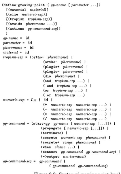
2 The Growing Point Language
2.1 Language Overview . . . . 2.1.1 The Concepts . . . . 2.1.2 Primitive Datatypes . . . .
2.1.3 Execution . . . . 2.2 Defining a Growing Point . . . . 2.2.1 Tropism Expressions . . . . 2.2.2 Growing Point Commands . . . .
2.2.3 Growing Point Expressions . . . . .
2.3 Abstractions and Methods of Combination.
2.3.1 Linking growing points . . . .
2.3.2 Aggregating growing points . . . . .
2.3.3 Network Commands . . . . 2.3.4 Auxiliary Commands . . . . 2.3.5 Aliases . . . .
2.4 The Execution Model . . . .
2.4.1 Justification for the Execution Model
2.5 Examples: Simple CMOS Circuit Layouts . 2.5.1 The Primitive Pieces . . . . 2.5.2 Building Bigger Abstractions . . . . 2.5.3 Generating Bigger Circuits . . . . .
2.6 Comments . . . . 2.6.1 Expressing Distances in GPL . . . . 2.6.2 Limited Tropisms . . . . 13 13 15 16 17 18 18 19 21 21 22 22 22 23 23 24 25 27 28 28 29 30 32 32 33 33 35 36 37 39 43 45 45 45
3 GPL: A Particle's Perspective
3.1 A Language of Local Rules . . . . 3.1.1 The Model for a Computational Particle . . .
3.1.2 A Simple Example . . . . 3.1.3 Abstractions . . . . 3.2 Translating GPL to ECOLI . . . . 3.3 The Representations of the Primitive Datatypes . . .
3.3.1 Pheromones . . . . 3.3.2 M aterials . . . . 3.3.3 Growing points . . . . 3.4 Translating Tropisms . . . . 3.4.1 Filtering . . . . 3.4.2 Sorting . . . . 3.5 Cooperation Dependent Commands . . . . 3.5.1 Secretions . . . .. . . . . 3.5.2 The Propagate Command . . . .
3.6 Communication-Independent Commands . . . .
3.6.1 Deferring Growing Points with Continuations 4 Theoretical and Practical Limitations of GPL
4.1 A Framework for Analysing GPL Programs . . . . .
4.1.1 Some Notation . . . . 4.1.2 Denoting GPL Computation . . . .
4.1.3 Some Basic Assumptions . . . .
4.1.4 Watching Resources . . . . 4.1.5 Analysing Rays and Line Segments . . . . 4.2 Implementing Arbitrary Networks with GPL . . . .
4.2.1 The Main Proposition . . . . 4.2.2 Overview of the Method . . . . 4.2.3 Proof Outline for Main Proposition . . . . 4.2.4 Code Definitions . . . . 4.2.5 Discussion of the Main Result . . . . 4.3 Analysis of Resource Usage . . . . 4.3.1 Static Memory . . . . 4.3.2 Dynamic Memory . . . . 4.3.3 T im e . . . .
4.3.4 Domain Space . . . . 4.4 The Effects of Random Distributions . . . . 4.4.1 Setting up the Domain . . . . 4.4.2 Characterizing the Domain
4.4.3 Domain Requirements for Good Propagation 4.4.4 Errors in Secretions . . . . 4.4.5 Summary . . . . 4.5 Bibliographic Notes . . . . 47 47 47 50 51 53 54 54 54 54 55 56 57 60 60 63 69 69 73 74 74 74 78 78 79 84 84 85 86 86 89 92 92 92 93 93 95 96 96 99 101 108 108 . . . .
.
.
.
.
5 Explorations in the Expressiveness of GPL 5.1 Generating Line Segments, Rays and Arcs . . . .
5.1.1 Generating Rays: Modeling Inertia . . . . 5.1.2 A rcs . . . .
5.2 Approximating Euclidean Constructions . . . . .
5.2.1 Translating the primitives . . . .
5.2.2 Combining the Primitives: An Example .
5.3 Drawing Circuit Layouts . . . . 5.3.1 A Library of Building Blocks . . . .
5.3.2 Preventing Unwanted Proximity . . . . .
5.3.3 Alternative Implementations . . . .
5.4 Looping Constructs . . . . 5.4.1 Repeating execution at a single location .
5.5 Biological Inspirations . . . .
5.5.1 Starfish . . . .. . . . . . .. . . . . 5.5.2 Trees . . . . 5.5.3 An Arm . . . . 5.6 Expressing Mirror Symmetric Forms . . . .
5.7 Sim ple Text . . . .
5.7.1 The initial conditions . . . .
5.7.2 Defining the strokes . . . .
5.7.3 Defining the Letters . . . .
5.8 Limitations of Network Abstractions . . . .
6 Conclusions and Future Work
6.1 Discussion of Results . . . .
6.2 Related Topics . . . .
6.3 Extensions to GPL . . . .
6.3.1 Other Tropisms . . . .
6.3.2 Time sensitivity . . . . 6.3.3 Denotable Growing Point Paths . . . . 6.4 Reliability Issues . . . . 6.4.1 Communication Errors . . . . 6.4.2 Increased Survivability of Growing Points 6.4.3 Incorrect computations . . . . 6.5 Extensions to ECOLI . . . . 6.5.1 The consequences of mobile particles . . . 6.5.2 Sensing and Actuation . . . .
6.6 Concluding Remarks . . . .
A GPL code listings
A.1 Lines and Arcs . . . .
A.1.1 Euclidean Construction . . . . A.2 CMOS Circuit Layouts . . . . A.3 Looping Constructs . . . .
A.4 Biological Inspirations . . . .
110 . . . . 110 . . . . 111 . . . . 113 . . . . 114 . . . . 115 . . . . 116 . . . . 117 . . . . 117 . . . . 120 . . . . 120 . . . . 121 . . . . 121 . . . . 122 . . . . 122 . . . . 124 . . . . 125 . . . . 128 . .. .. .. . 129 . . . . 130 . . . . 131 . . . . 132 . . . . 133 136 . . . . 136 . . . . 137 . . . . 138 . . . . 138 . . . . 140 . . . . 142 . . . . 143 . . . . 144 . . . . 144 . . . . 145 . . . . 145 . . . . 145 . . . . 146 . . . . 146 148 . . . . 148 . . . . 152 . . . . 154 . . . . 173 . . . . 174
B ECOL1 Implementation of Secretion FSM 184
B.1 The FSM Definition ... . 184
B.2 Implementation of secrete ... 187
B.3
FSM s in ECOLI ... 190B.3.1 Support code ... . 190
B.3.2 Generator for Secretion FSM ... ... 192
B.4 Support code for pheromone maintenance . . . . 195
B.5 Runtim e Utilities . . . . 198
C Implementation of the GPL illustrator 203 C.1 Interpreter code . . . . 203
C.1.1 Top Level commands . . . . 203
C.1.2 Growing point commands . . . . 208
C.1.3 Network commands . . . . 216
C.1.4 Tropism Implementation . . . . 220
C.2 Domain Implementation . . . . 227
List of Figures
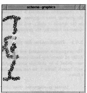
1-1 A large non-trivial pattern expressed by GPL . . . . 14
1-2 A topologically constrained pattern . . . . 15
1-3 The realization of that pattern on the system of elements . . . . 15
2-1 Tropism directions . . . . 26
2-2 Syntax of growing point level commands . . . . 34
2-3 The syntax of network level GPL commands . . . . 34
2-4 The CMOS Layout of an inverter . . . . 36
2-5 The CMOS Layout of an inverter on a randomly arranged domain . . . . . 36
2-6 The Steps in the Formation of the Layout of a CMOS Inverter . . . . 42
2-7 The CMOS Layout of a NAND gate . . . . 43
2-8 The CMOS Layout of an NAND gate on a randomly arranged domain . . . . 43
2-9 The CMOS Layout of an AND gate . . . . 45
2-10 The CMOS Layout of an AND gate on a randomly arranged domain . . . . 45
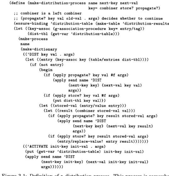
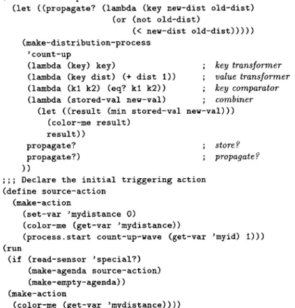
3-1 Definition of a distribution process. This process is somewhat like a list accumulation in Scheme. . . . . 51
3-2 Count-up waves implemented using the distribution abstraction . . . . 52
3-3 Tropism Architecture . . . . 55
3-4 FSM for controlling a particle's reaction to messages generated during the secretion process. . . . . 61
3-5 FSM for controlling the pheromone source's reaction to messages generated during the secretion process . . . . 62
4-1 Sketch of the grid layout of a planar graph . . . . 74
4-2 Illustration of definitions . . . . 77
4-3 Propagation of the ray growing point . . . . 82
4-4 Smallest possible angle attainable on an n - 1 by 2n - 4 grid. . . . . 93
4-5 Computation of s(uv) given 9 . . . . 93
4-6 An arbitrary region in the GPL domain, with one of its cells shaded. . . . . 96
4-7 Propagation direction accuracy . . . . 99
4-8 Secretion of extent 10. Darker greys indicate lower pheromone values . . . . 102
4-9 Same secretion of extent 10 but with errors highlighted in blue (dark grey if no colour) . . . . . 102
4-10 Scatter plot of secretion levels vs. Euclidean distance from the source . . . 103
4-11 A bad shortest path . . . . 104 4-12 Scatter plot showing variation of secretion errors with average variance of
5-1 A GPL construction of 60 . . . . . 117
5-2 Invoking ray 5 times at the same point. . . . . 122
5-3 Invoking ray 7 times at the same point. . . . . 122
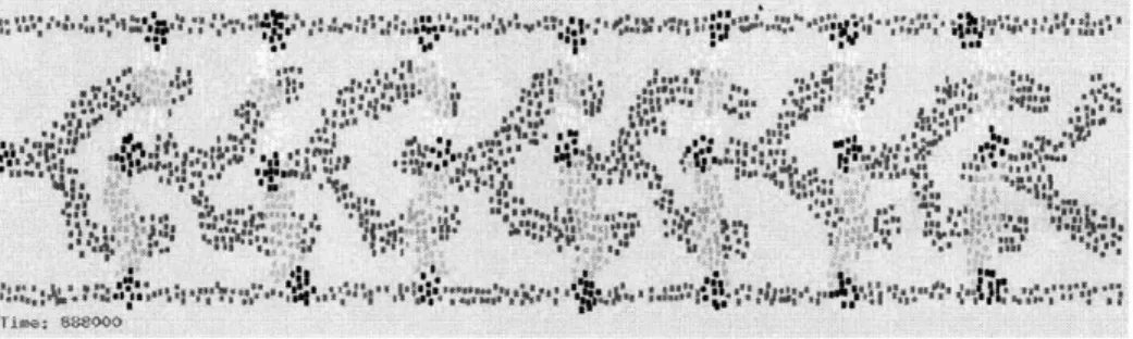
5-4 A starfish, as interpreted by GPL. . . . . 123
5-5 A tree with branch factor 3. Notice how the locations around each branch point are relatively evenly spaced, because each side branch repels the other as much as the trunk repels each of them. . . . . 124
5-6 A tree with branch factor 3. Each new side branch is pushed away from the trunk more than from each other, as indicated by the bunching up of locations in the trajectory near the point of bifurcation. . . . . 124
5-7 A hand, rendered by GPL on a regular grid with a Euclidean metric. . . . . 126
5-8 The same hand rendered on an irregular particle distribution with a shortest-path m etric . . . . 126
5-9 A pair of hands generated by mirroring the code for a single hand. . . . . . 129
5-10 The same program rendered on an irregular particle distribution with the shortest-path metric . . . . 129
5-11 Text expressed in GPL. . . . . 130 5-12 Sector looks bad for short arc lengths because of superposition of pheromones. 135 5-13 Sector looks better for the same initial conditions, but a different arc length. 135
List of Tables
2.1 A list of aliases for GPL keywords . . . . 33
4.1 The code sizes for the growing point definitions used in the construction. . . 92
4.2 Selected data showing trends in the neighbourhood sizes and the number of errors in the pheromone levels. . . . . 105
4.3 Selected data showing trends in secretion errors and in the Euclidean dis-tances between neighbours. . . . . 106
Chapter 1
Introduction
The cells of an embryo specialize and develop under the control of a common genetic pro-gram housed in each cell. The organism that forms is almost always correctly formed: the appropriate body parts are present and are connected appropriately. By what means is the morphology of the organism expressed in its genetic code? How do two distantly separated cells specialize in different ways to perform different tasks, despite the fact that they are independently directed by identical genetic programs?
This dissertation presents a programming paradigm and an implemented programming language that can control a programming environment that is similar to a collection of interacting biological cells. Specifically, assume that we are given a system of myriad com-putational elements, irregularly placed, interacting only locally, and asynchronously run-ning identical programs. I present the Growing Point Language (GPL) for specifying the construction of interconnect topologies on that system. A GPL program is expressed in terms of concepts that are meaningful only when the system is regarded as a single pro-grammable entity. Yet when that program is interpreted simultaneously on every element of the system-in much the same way that the cells of any embryo "execute" their common ge-netic program-it is capable of producing prespecified effects that may involve coordinated differentiation (of behaviour) on distantly separated elements.
The principal concept in GPL is the growing point. It is a locus of activity that describes a path through connected elements in the system. A growing point propagates through the system by transferring its activity from one computing element to a neighbour. As a growing point passes through the system, it effects the differentiation of the behaviours of the elements it visits. The trajectory of the growing point is controlled by signals that are
automatically carried through the system from other differentiated elements.
The work presented here is not an attempt to model biological processes. The goal is to try to understand, from an engineering perspective, how macroscopic properties of a system arise from microscopic perturbations that take place within it. Specifically, we want to know when given a macroscopic goal, what microscopic actions ought to be prescribed
in order to achieve it.
1.0.1 The Growing Point Language
The implementation of GPL rises to this challenge by providing a means of expressing logical global topological constraints that can be enforced through local interactions by exploiting interconnect geometry. We are able to specify non-trivial topologically constrained patterns from a modest number of initial conditions via a GPL program. Figure 1-1 shows an example
Figure 1-1: Each rectangle represents a computational element. Each one is coloured ac-cording to a value maintained in the element's state. The size of a neighbourhood is the thickness of one of the interior lines.
of such a pattern, which was obtained from a small program encoding about seventeen computational states. The initial conditions included the two shaded lines at the top and bottom of the pattern and a single point at the left edge.
By implementing an interpreter that translates system-level GPL commands to
element-level instructions, we provide insight into the relationship between emergent macroscopic properties and microscopic actions. Our implementation makes minimalist assumptions about the computational capabilities of the system elements. Therefore, by exhibiting topologically constrained patterns like that in Figure 1-1 we demonstrate that the necessary conditions for controlling such global organization are few.
The GPL system translates a GPL program into code fragments that are executed on each computational element by a message-passing event driven loop. Since the method of translation is oblivious to the identity of the element that eventually runs the code, every
element inherits identical code fragments. However, as can be seen from Figure 1-1 some
elements must eventually assume different states from others.
The problem then is to generate code fragments that will differentiate, in a controlled way, the behaviour of each element they run on. That differentiation can be controlled in two ways: in response to changes in local state on the element, or in response to messages received by the element. Therefore, the behavioural differentiation at each element must be highly coordinated in order to meet the non-local constraints originally expressed by the GPL program.
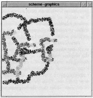
Figure 1-2 illustrates a pattern whose essential feature is the connectivity of the lines in it. We call this pattern topologically constrained. Figure 1-3 illustrates what it means for the system to draw the pattern shown in Figure 1-2. Each disc represents a system element, and each colour represents a label that the element has assigned itself during the drawing computation. Connected regions of common labels can be mapped, via the colour codings shown, to regions in the given pattern in Figure 1-2 in a way that preserves its topology. The pattern in Figure 1-2 represents an example of the type of patterns that GPL is capable of expressing.
We make two claims:
e Strictly local communication and a common program are sufficient conditions to
Figure 1-2: A topologically constrained Figure 1-3: The realization of that
pat-pattern tern on the system of elements
e The interconnect topology of any planar graph is expressible as a GPL program.
Thesis:
Any planar interconnect topology can be drawn by a system of irregularly con-nected, identically programmed, asynchronous, locally-interacting computational elements.
1.0.2 Context
One broad example of the endeavour to control macroscopic effects through the direction of microscopic action is genetic engineering. There, biologists attempt to obtain a specific phenotypic property (for example, improved resistance to disease) by genetic manipulations.
A good specific example of work that shares our goals is Slack's theory of morphology.
Slack [46] presents a description of how the morphology of an organism might be designed
by manipulating its genes.
The point here is that we want to learn how to actively control global behaviours when we have access to only local manipulations. Under ideal conditions, we fully understand the effect of each local manipulation, and so we can focus on understanding the nature and origins of the emergent properties of the system. In the case of genetic engineering, we do not fully understand the effects of every primitive operation, so the problem of controlling emergence is compounded. We are hindered from gaining as much insight into our problem than would be the case if we had a complete understanding of all the local operations.
Unfortunately, there are few synthetic examples of research with similar goals to ours. One example from distributed control theory is research to show that the shape of a stressed beam can be controlled using sensors and actuators that are distributed along the length of the beam [21, 24, 7]. Other examples are in computational modeling of biological processes:
9 A Lindenmayer system [43] hybridized with diffusion can be programmed (by local
* A lattice model of protein folding has been used to investigate the complexity of the inverse protein folding problem [55]. The inverse folding problem attempts to find a sequence of residues that will fold to some given target native conformation.
In each of these three examples there is a global goal that must be achieved as a result of local actions. So in that respect, they are similar to the work we present.
There are at least two important differences between these examples and the approach described in this dissertation. The first is that all of those examples used regular discretiza-tions of space. The second difference is that none of those examples had as strict locality constraints as we do. For example, in the beam controller, actuation decisions were made with complete global knowledge, and in the model for axonal growth, arbitrary angles could be specified at any location which implied an implicit global coordinate frame. In all of those examples, a physical system was being modeled, so it made sense to facilitate the analysis
by making the discretization of space regular or permitting non-local computations when
necessary. In this dissertation, we are primarily concerned with the organizational princi-ples involved in controlling a large system of loosely coupled, locally interacting elements. We do not assume that these elements are regularly arranged (without precluding the pos-sibility that they are), and we strictly enforce the locality constraints for communication
and computation on the elements.
In this respect, our goals are more aligned with those of Distributed Computing [34, 31], where the primary concern is how to coordinate the operation of networks of computers. However, in Amorphous Computing, we retain the concept of space to limit the types of connections that can be made between the system elements. Therefore the setting for this dissertation is unique: we do not claim to model any particular physical system, yet we retain physical spatial constraints in determining the interconnect of the system. In general, we seek to understand how geometric constraints on a large system's elements may be exploited to effectively control the global behaviour of the system.
1.0.3 Motivations
Given the recent advances in Biotechnology and microfabrication technologies, we may soon have programming access to large systems of computational elements. The numbers of el-ements would be enormous, significantly larger than any system we currently have. These elements might be realised as biological cells or more familiar silicon-based hardware; but they will, of necessity, be small and therefore resource-limited. It is also prudent to as-sume that they will probably be unreliable and loosely coupled in irregular interconnection networks. If we were given such a system today, we would be hard-pressed to do its com-putational power any justice, not because we lack difficult tasks, but because we lack the understanding to deal with such a system.
The study of Amorphous Computing addresses this problem by researching techniques that enable us to engineer useful system-wide behaviours. In order to develop our ideas on differentiating local behaviour to obtain globally coherent goals, we needed to solve a more specific problem. We chose the generation of patterns of interconnect topologies as our model global behaviour because:
3. it represents an unprecedented level of control over macroscopic properties derived
from the manipulation of microscopic parameters.
Ultimately we would like to learn and understand general principles that will aid us in controlling immensely complex systems. We believe that such systems are imminent. Therefore it is extremely important for us to discover new ways of reasoning that will allow us to properly marshal their resources. Such novel reasoning techniques will undoubtedly involve abstractions that present a simple interface to the system. But these techniques must go one step further to include the automatic implementation of the interface through cooperation of the elements. By studying a non-trivial problem such as interconnect topol-ogy layout generation, we hope to gain some insights into the nature of that interface and its implementation.
1.1
The Amorphous Computing Model
An amorphous computer consists of myriad computing particles embedded in physical space. The particles have limited memory and modest computational resources; they run asyn-chronously, communicate with each other over a very limited physical distance, and are placed arbitrarily with respect to each other. We assume that the receivers on each particle are omni-directional and therefore a particle cannot immediately determine the relative lo-cation of a transmitting neighbour. The large number of particles precludes programming each one individually. Therefore, the programs executed by these particles are constrained to be initally identical (although the programs may contain multiple entry points). At the beginning of a computation, the only way to distinguish a particle from the rest is to give it a different entry point into the common program. Subsequent variation in behaviours among the particles must be self-induced: whether by communication with neighbours, by sensory input values or by random numbers.
The model considered here further constrains the particles to be static. So their in-terconnect, although unknown a priori, is fixed for the duration of any computation. The message of a single transmission must be shorter than a statically specified number of bits. Messages take time to deliver, during which a particle is allowed to continue computing. Each particle is built to encode and decode messages in exactly the same way. Therefore, the low-level communication protocol is not subject to software controlled variation (this does not preclude a particle from dynamically adjusting the manner in which it interprets the information in a message). The details of the programming language that we shall use for these devices are presented in Chapter 3.
The types of global behaviour that we consider will be restricted to those that specify a goal pattern for the system to assume. If the system were the collection of cells of an embryo, an example of this type of global behaviour would be the connectedness of the organism. Since the particles in this amorphous computing model are static, the computing particles assign themselves labels to correspond to features in the given specification of the goal pattern. Regions in the space of locations of the particles are determined by connected particles of common labels. A labeling is successful if there is a topology-preserving map from the regions obtained from labeling and the given pattern.
1.1.1
Justification for the Model
The physical realization of the computational elements determines the representation of our computations, and therefore the kinds of operations that will be convenient to perform. For example, if our elements are biological cells, then our computational states and data may be represented by chemical concentrations of various signal substances. If our devices are even smaller, say molecules, then our states and signals might be represented by electron distributions. It is already a bold assumption that we might be able to manipulate these microscopic elements in the way we manipulate computers. So it is only natural that we choose to restrict the resources available to each computational element.
We have taken a minimalist view of the capabilities of our computational particles so that our results will be general and robust. We do not assume that a particle can detect the direction from which a received message came, even though it is conceivable that that might be possible (for example, if our particles are cells and the messages are chemicals that attach to the cell's membrane). The assumption that particles have restricted resources encourages us to develop scalable algorithms that rely on only local cooperation among the particles. Regarding the initial conditions, while we assume that we can statically manipulate these particles arbitrarily, we do not want to extend that assumption to dynamic, real-time ma-nipulation. For that reason, we constrain the model to accept external intervention only when the initial conditions need to be setup. Everything else should be autonomous, that is directed by the program.
Even the assumption that the particles are computationally equivalent to space-bound Turing machines may be too strong. Indeed, our results indicate that for the purposes of the problem addressed by this thesis, we may not need to assume as much computational power as a space-bound Turing machine. However, we chose to start with that assumption so that we could focus on the real issues at hand: moderating the interactions between the elements in an orderly manner, and doing so with a control specification that is initially identical on each device.
1.2
Encoding Patterns
Suppose that we are given the pattern in Figure 1-2 to draw on our amorphous computer. To simplify the problem, suppose also that the system has already been initialized so that the elements coloured blue (those comprising the two lines at the top and bottom of Figure
1-3) have already been labeled. We are also given one element on the left from which we
would like to produce a pattern of labelings on the elements that has the topology of that in Figure 1-2. How do we think about organizing such a pattern, when we know that the elements have no (explicit) information about their locations, and that for them the concept of "direction" will need to be defined?
For the moment, let us ignore the second problem, and imagine how we would generate the pattern, obeying only the locality constraints. That is, we are allowed to draw a new point or line only if it is next to a point or line already drawn. We might proceed as follows:
1. Draw a short length of red line parallel to the given blue lines, which we will refer to
here as "rails".
3. From the end of each of those new red lines, draw another short red line parallel to
the rails, and away from the original starting point on the left.
4. On each of the parallel red lines, near its end, draw four vertical lines, two in opposite directions towards the rails, and two in opposite directions towards each other. Use yellow for the segments near the top rail and green for the other two near the bottom rail.
5. Where each of the new vertical lines intersects with a rail, place a black rectangle
there.
6. Where the yellow and green lines intersect, place a black rectangle there and draw a
short red line away from the original starting point.
Upon even a cursory examination of the steps outlined, it is clear that the ability to draw a line in an arbitrary direction with a controlled length is a very useful subroutine to have. In fact, the only remaining problem given such a subroutine would be the matter of sequencing the calls to the subroutine so that the lines are drawn according to the plan. However those two steps represent significant issues that need to be addressed in this computational environment:
" What do terms like parallel, towards and away from mean to an element, for which
there is only the concept of immediate connectivity to other elements?
" All the elements have the same program. So how will the ones that comprise a line
that we draw be distinguished from those off the line?
" All the elements are executing asynchronously in parallel. So even if they are able to
coordinate a line pattern, how do they ensure that those lines are connected appro-priately?
A GPL program allows the user to express a pattern in a manner like the steps of the
outline above. It hides the underlying issues from the user, so that the user can think in terms of the elements of the pattern being expressed. It can denote only points that have already been drawn or that were given in the initial conditions, thereby enforcing the locality constraint.
A line is readily expressed as the trajectory of a growing point that tries to take the
most direct route to its destination. Growing points can cause the execution of instructions at the particles that house them. In this way growing points can invoke other growing points, and perform operations that affect other growing points. These properties can be used as a serializing mechanism to ensure that the patterns we express are connected appropriately. For example, to draw one line from the end of another, we cause the growing point responsible for the first line invoke the second growing point. Growing points can be named and invoked multiple times, so the user can effectively abstract commonalities in the given pattern.
1.3
How GPL works
Let us take a close look at the implementation of a simple program to draw a line segment between two points.
(define-growing-point (A-to-B-segment) (material A-material)
(size 0)
(tropism (ortho+ B-pheromone)) (actions
(when ((sensing? B-material) (terminate))
(default
(propagate)))))
The definition of a growing point has two parts: the attributes and the instructions. The attributes section describes the type of material (if any) that is deposited, the thickness of the curve produced and the rule for determining the next location for the growing point. In this example, the name of the growing point is A-to-B-segment, it deposits a material (i.e. sets a logical marker) called A-material, it has zero width (so the trajectory will be as thick as the size of a particle) and it grows towards increasing quantities of a signal called B-pheromone (the meaning of positive orthotropism for B-pheromone).
The instructions section of a growing point definition contains a sequence of commands that are executed at each location visited by the growing point. These commands control whether the growing point moves or not, whether it secretes any pheromones, and whether other growing points get initiated or not. In the example, the growing point will stop moving if there is any of a material called B-material deposited at its current location. Otherwise, it tries to move to some point in the immediate neighbourhood of its current location. Note that while the commands may control whether a growing point moves or not, it is the tropism declaration that controls how the growing point moves when it does. As its name implies, the example is a fragment of GPL code for drawing a directed line segment between two points. If we label two points in the plane A and B (as the name suggests) then we would want to initiate A-to-B-segment at the point A. However, as it is written, A-to-B-segment will need some help to actually produce the desired line segment; there must be some cooperation from the point B. Here is some more of the GPL code:
(define-growing-point (B-point) (material B-material)
(size 0) (for-each-step
(secrete 10 B-pheromone)))
This code fragment defines another growing point named B-point which deposits mark-ers called B-material and has zero width. Also quite importantly, B-point does not have a tropism declaration which means that it is stationary. The body of B-point introduces the secrete command. Its effect is to distribute a signal called B-pheromone radially symmet-rically, with monotonic decreasing strength, for up to 10 units away from B-point's current location.
Now we see how A-to-B-segment and B-point interact: since B-point is the source of all B-pheromone, any A-to-B-segment located within 10 units of B-point will grow towards it. Since the growth of A-to-B-segment is specified to be positively orthotropic to (ie. "directly towards") B-pheromone, and the pattern of distribution of pheromones is radially symmetric, the resulting path of the original active site of A-to-B-segment to B-point is a straight line.
fore take arguments when invoked. It so happens that both growing points in our example do not have any parameters, but we will see later how growing point parameters allow active sites to communicate information non locally so that we can produce curves of a particular
length, or with varying sizes.
1.4
What GPL builds on
The GPL system is actually two systems at different levels. There is the lower level that models the system's particles and their interactions, and there is the higher level which implements the GPL interpreter.
The models for communications at the lower level were founded on models that were originally used for packet radio networks [38]. Our models evolved from explicit simulations of actual protocols like ALOHA (see [47] for a description) to the more abstract, layered model in the end (which was inspired largely by the organizational layers of the ISO OSI model and TCP/IP). Our model for computation is based on an event-driven that is closely coupled with the message-passing communications model [31].
The techniques for implementing secretions are based in part on approximations to simu-lations of diffusion. Our first implementations arose from our efforts to establish amorphous coordinate systems [13] and later from simulations of the Gray-Scott model of reaction-diffusion [42, 14]. Conversations with Norm Margolus and Raissa D'Souza about reaction-diffusion on cellular automata led to a better understanding of the time complexity involved and consequently a different time-accuracy tradeoff in our implementation. For analytical treat-ments of the problem, we turned to several sources [33, 11, 8], most notably Ahlfor's text [3]. At the higher level, much of our implementation of GPL is reminiscent of the meta-circular evaluator and Scheme compiler presented in Abelson and Sussman's text [1]. Un-published course notes from the Programming Languages class at MIT, 6.821 [20] also contributed in important ways.
1.5
Outline
Chapter 2 is a detailed description of GPL and presents a more elaborate description of the program for expressing the pattern from Figure 1-2. Chapter 3 describes the message passing language used by the particles, and presents the translation process from GPL to that language.
Chapter 4 presents some analysis for GPL. The first part presents a framework for analysing GPL programs in general, and presents some analysis for two common building block growing points, namely rays and line segments. The next part of the chapter demon-strates that any planar graph is expressible in GPL, and discusses the resources involved in realising it. The last part of the chapter presents some empirical data for characterising the dependence of the success of GPL programs on the distribution of particles in the system.
Chapter 5 presents a range of patterns that are expressible in GPL. It also highlights some of the interesting programming paradigms within GPL. Finally, Chapter 6 presents our conclusions and outlines the future directions for this research.
Chapter 2
The Growing Point Language
This chapter describes the Growing Point Language in detail. Throughout the presentation, we use code excerpts from a single example pattern to illustrate the particular language feature under discussion. Finally, we try to characterise the types of curves that can be constructed in GPL. Complete code listings for the GPL interpreter are given in appendix C. The Growing Point Language (GPL) is a programming language for specifying intercon-nect topologies in a coordinate-free way. The behaviour of a GPL program is determined
by its text, an associated domain and a set of initial conditions. The GPL domain
con-sists of a set of points, a metric for defining distances between them, and a characteristic distance called the step-size. The members of the GPL domain are referred to as locations within the language, and will be referred to similarly from now on. The initial conditions are specified as associations of locations (i.e. points from the GPL domain) with program commands. The specification is done in the program text with abstractly denoted locations whose actual values are supplied when the GPL program is evaluated.
2.1
Language Overview
Before plunging into the details of GPL, we present a brief overview of the language, and describe the principal concepts at an abstract level.
2.1.1 The Concepts
A growing point is a locus of activity that describes a path in the GPL domain. At any given
moment, a typical growing point is housed at a single location in the GPL domain, called its active site. A growing point may "move" in discrete steps in the domain according to its tropism by changing its active site from one location to a neighbouring location. At its active site, a growing point may "deposit" material and it may "secrete" pheromones. (Both processes are, in fact, associations of locations in the GPL domain with values to represent either the presence of a material (deposition) or the quantity of a pheromone (secretion).) The tropism of a growing point is specified in terms of differences in pheromone levels in the neighbourhood of the active site. Specifically, the pheromone quantities form a scalar field whose gradient directs the motion of the growing point. The path that the growing point describes is the collection of locations that it has visited. The path is detectable only
coordinates in the plane. The correspondence between types of materials and types of pattern fragments is established before the program is executed. In this way a GPL program draws a definite pattern that can be recognized based on only the proximity of common types of material deposits.
The definition of a growing point dictates the topology of its path, however the geometry of a particular path that a growing point produces-being dependent on the geometry of the domain-is determined only after the growing point has been invoked at some location. Invoking a growing point at a location may yield successor locations in the domain. If there are no successor locations, the growing point terminates the path at that location; otherwise each successor location in the domain is not farther than step-size from the current active site. In most cases, there is at most one successor location to an active site, so the path produced is simply a polygonal path. In cases where there are more than one successor locations, then the "path" is actually a tree in the GPL domain. Whether we have a tree or a polygonal path, each edge connects locations that are neighbours in the GPL domain. The step-size is the fundamental unit distance: it defines a growing point's neighbourhood; it is therefore an upper bound on the size of every growing point's step; and it is also used as the unit by which all distances in GPL are expressed.
2.1.2 Primitive Datatypes
There are two types of primitive objects in GPL: pheromones and materials.
Materials are used as markers to indicate where growing points have previously visited. The color command associates a material type with a colour which is used to highlight locations as they are visited. Materials can also be sensed by growing points so that de-cisions for growth may be based on what materials have already been deposited at a site. Ultimately, it is in the arrangement of the materials deposited that we will look to find the pattern we intended to generate.
Pheromones exist to guide the movement of growing points. Pheromones are produced when a secrete (or secrete+) command is executed. The extent of the surface to be covered by the pheromone is also specified in the command. The distribution of pheromone quantities is radially symmetric about the source, and monotonic decreasing in the distance from the source. The exact shape of the distribution is deliberately unspecified and should not be depended upon by GPL programs.
2.1.3 Execution
As part of their definition, growing points embody commands that must be executed at their active sites. Commands in the body of a growing point's definition are evaluated in sequence by the particle at the growing point's active site. Each command must complete before the subsequent command in sequence is executed. For most commands, completion simply means that the operations associated with that command have all been executed successfully. A few commands require communication between the active site and locations near it. For these, completion means that the operations associated with that command have been executed successfully not only at the active site, but also on every location that was involved in the processing of the command. These commands rely on completion
messages from the neighbouring locations to the active site. So usually the active site must wait for an indication that the next command may be evaluated.
An active site executes until either it encounters a halt or terminate command, or it runs out of commands to evaluate. When a new active site is spawned, the original one may not have finished evaluating all of its commands. In this case, both active sites are considered to be processing commands in parallel. The spawning active site pauses for a short period after the new active site has been spawned. There are no commands to explicitly control the rate at which an active site processes commands. So this implicit pause is a mechanism to allow the second active site to begin execution and possibly affect
the first active site's subsequent computation.
When a growing point moves, it requires the presence of at least one pheromone to guide its motion. If at such a time there is no relevant pheromone present at the active site, the active site is stalled until that pheromone becomes detectable. If however, the appropriate pheromones are present, but no acceptable location can be found to move the active site to, then the active site retries. After three failures to find an acceptable location, the active site halts execution, and the growing point is stuck.
2.2
Defining a Growing Point
Rather than give a formal definition and syntax for all the features of GPL, we will present small code examples that will exercise many of those features. Growing points are created with the define-growing-point command. Here is an example of its use.
(define-growing-point (orient-poly length)
(material poly) (size N-WIDTH)
(tropism (and (ortho- dir-pheromone)
(and (dia vdd-long) (dia vss-long)))) (avoids poly-id-B) (actions (secrete 2 poly-id-A) (secrete+ 3 poly-pheromone) (when ((< length 1) (terminate)) (default (propagate (- length 1))))))
A growing point has a name, orient-poly in this case; it may have parameters, length
is the only one here; and it may have any or all of several attributes, indicated by the keywords: material, size, tropism, avoids, actions. The name is used for referencing the growing point and is scoped globally since all growing point definitions are at the top-level. Any parameters, on the other hand, are scoped over the definition of the growing point. Parameter values may be either numbers or boolean values.
The material attribute designates the tag that is associated with each location that the growing point visits. The value of this tag must be a constant literal. Each location keeps a list of material tags that can be polled by growing points visiting that location. This "detection" of materials allows growing points to be sensitive to the presence of certain materials. It is important to note that a growing point does not deposit its material until
The material tags are also used as keys for colour-coding the growing point when the program's pattern is displayed. If the material attribute is unspecified, then the growing point does not cause any tag to be associated with the locations it visits; consequently its path cannot be displayed.
The size attribute indicates the half-width, in step-size units, of the growing point; it can be specified as any integer valued expression. The expression is evaluated once per invocation of the growing point and retains its value for the lifetime of the growing point (i.e. until it terminates). That value is used as the radius of the neighbourhood, in step-size units, with which the material tag will be associated. In the example, N-WIDTH is a globally specified constant, which happens to have the value 1. This means that when orient-poly is invoked, every point in the 1-hop neighbourhood of its location will be associated with the material tag. From the standpoint of the display, the growing point will produce a curve whose width is twice the step-size. If the size attribute is omitted then the growing point assumes the default size of zero. This means that only the location of the growing point will be tagged by the material tag, but not any of its neighbours.
The tropism attribute determines the pheromones to which the growing point is sensitive, as well as in what manner. The specification of this attribute is a tropism expression. Since tropism expressions have slightly involved semantics, we defer their detailed discussion for now. In this example, the tropism expression indicates that there are three pheromones of interest, their names are: dir-pheromone, vdd-long and vss-long. When the growing point is ready to change locations, the most favoured destination is the one that is furthest from the source of dir-pheromone (i.e. negatively orthotropic to dir-pheromone) yet also at distances from vdd-long and vss-long respectively similar to those of the current location (i.e. diatropic to vdd-long vss-long). Omitting this attribute implicitly implies that the growing point is stationary. In that case, use of the propagate (see description in section 2.2.2) command in the actions attribute is forbidden.
The avoids attribute indicates which pheromones inhibit the growing point. A growing point will never visit a location where any of the pheromones mentioned in this attribute are present. If this attribute is omitted, then no pheromones inhibit the growing point.
The actions attribute describes the sequence of commands executed at each location visited by the growing point. These commands control whether the growing point moves or not, whether it secretes any pheromones, and whether other growing points get invoked. In the example, the growing point will stop moving if the value of the length parameter is smaller than 1. Otherwise it attempts to visit another location (determined by the tropism attribute) where the value of the length parameter will be one less than its value at the current location. Note that while the commands may control whether a growing point moves or not, it is the tropism declaration that controls how it moves when it does. Growing points that are specified without an actions attribute implicitly terminate themselves when invoked.
2.2.1 Tropism Expressions
A tropism describes how a growing point moves. It is always expressed in terms of one or
more pheromones. A tropism expression is represented as a pair of a filter and a sorter that given a set of associations from neighbour ids to pheromone concentrations, returns a subset of acceptable associations, ordered from most acceptable to least acceptable. In order for a growing point to change its location, the values (concentrations) for the ap-propriate pheromones are polled from its location's neighbourhood, and filtered according
ortho+
ortho-plagio+
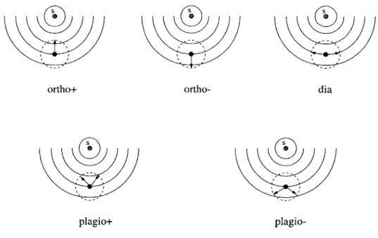
plagio-Figure 2-1: The directions, relative to the source of a pheromone, represented by each tropism expression. The particle marked 's' is the source of secretion. The arcs represent contours of the pheromone concentration. The dotted circle represents the neighbourhood of the active site, which is represented as a black dot. The arrows should be interpreted relative to the line joining the source and the active site.
to its tropism. The location associated with the first of the remaining (ordered) values is selected as the growing point's destination. If there are no values left after filtering, then the growing point is stuck and terminates at its current location. Tropism expressions have five primitive forms (ortho+, ortho-, plagio+, plagio- and dia) and four combining forms
(and, ~and, or, and -or). The primitive forms are described below'. Figure 2-1 illustrates
the directions that each tropism expression represents relative to the pheromone source. ortho+ : retain all pheromone concentrations higher than the current value, and give
preference in decreasing order of concentration. Rough interpretation: move in the direction of maximal increase of pheromone concentration.
ortho- : retain all pheromone concentrations lower than the current value, and give prefer-ence in increasing order of concentration. Rough interpretation: move in the direction of maximal decrease of pheromone concentration.
plagio+ : retain all pheromone concentrations higher than the current value; compute the average of the highest and the current concentration and give preference in increasing order of proximity of the concentrations to that value. Rough interpretation: move in a direction oblique to the direction of maximal increase of pheromone concentration. plagio- : retain all pheromone concentrations lower than the current value; compute the
average of the lowest and the current concentration and give preference in increasing dia
order of proximity of the concentrations to that value. Rough interpretation: move in a direction oblique to the direction of maximal decrease of pheromone concentration. dia : compute the range of pheromone concentrations and retain all those that differ from the initial concentration by less than a small fraction of the range. Preference is given in increasing order of proximity to the initial concentration. Rough interpretation: move in a direction orthogonal to the direction of maximal increase of pheromone concentration.
The combining forms take arbitrarily many tropism expressions as arguments. They must combine both the filtering and the ordering operations of each of their argument expressions to produce a single filter and a single sorter. The ordering operations are combined in the same way for each combining form. Suppose the sorters obtained from the argument expressions of a combining form are si and s2. The combined sorter gives
precedence to si, then uses s2 to order elements whose ordering was indeterminate under si. The method is best described in terms of the predicates used by these ordering operations. Say pred1 and pred2 are the respective predicates corresponding to si and S2, then the predicate corresponding to their combined sorter is
(lambda (elti elt2) (or (predi elti elt2)
(and (not (predi elt2 elti)) (pred2 elti elt2))))
Unlike sorters, filters may be combined in a number of ways, depending on the combining form specified. The compound filter for each combining form is described as follows:
and : compose the filters sequentially, using the output of one as the input to the next.
~and : compose the filters sequentially, as in the case of and, but only use as many beyond the first as possible that still return a non-empty result.
or : apply each filter in turn to the input set and return the first non-empty result. ~or : return the union of the result of each filter applied independently to the input set.
2.2.2 Growing Point Commands
All GPL commands begin with a keyword. It may be followed by appropriate arguments
depending on the command. A command sequence is simply a list of commands, no special keyword is required to indicate one. Here is a description of all the commands2 that may be used within the actions attribute. Recall that these commands are executed only when a growing point is invoked at a location, therefore it always makes sense to talk about the current location in the context of their explanations.
(start-gp < gp-name > < argi > ... ) Invoke the growing point named by gp-name at the current location. The given arguments are supplied as the initial values of the parameters declared in the definition of gp-name.
2
(propagate < argi > ... ) Find a new location for the growing point, propagate all its dynamic state including the new values for the parameters given by the values of argi, and invoke the command sequence of the actions attribute at the new location. (terminate) Terminate the growing point at the current location.
(secrete < range > < pheromone > ) Secrete enough of the pheromone named pheromone
so that its concentration is monotonic decreasing from the source and zero at a distance
range from the current location. The concentration at the current location depends
on the value of range. The pheromone concentration recorded at each affected site is taken to be the larger of its current value for pheromone and the quantity arriving there due to this secretion.
(secrete+ < range > < pheromone > ) Secrete enough of the pheromone named pheromone so that its concentration is monotonic decreasing from the source and zero at a dis-tance range from the current location. The concentration at the current location depends on the value of range. The pheromone concentration recorded at each af-fected site is taken to be the sum of its current value for pheromone and the quantity arriving there due to this secretion.
(when < clause1 > ... (default
<
default-seq > )) Each clause consists of an expressionfollowed by a command or a command sequence. Each clause's expression is evaluated in turn until one of them evaluates to a non-false value. When that happens, the associated command or command sequence within the containing clause is executed. The special expression default always evaluates to true. Upon completion of the execution of a command sequence of a clause, execution returns to the point after the when command.
2.2.3 Growing Point Expressions
All expressions must evaluate to either numbers or boolean values. They may be: " literal numeric constants
e variables such as parameter names, growing point names and globally declared con-stants.
" arithmetic expressions combining any of the arithmetic operators +,-,*,/ with numer-ically valued expressions.
" logical comparisons using one of the arithmetic comparators <, =, >.
" (sensing? material-name ). This expression returns true if the tag material-name has previously been associated with the current location.
2.3
Abstractions and Methods of Combination
The commands presented so far are sufficient to render any given topology in the GPL domain. However, as yet there are no ways of capturing common patterns in growing