HAL Id: hal-00442763
https://hal.archives-ouvertes.fr/hal-00442763
Submitted on 22 Dec 2009
HAL is a multi-disciplinary open access
archive for the deposit and dissemination of
sci-entific research documents, whether they are
pub-lished or not. The documents may come from
teaching and research institutions in France or
abroad, or from public or private research centers.
L’archive ouverte pluridisciplinaire HAL, est
destinée au dépôt et à la diffusion de documents
scientifiques de niveau recherche, publiés ou non,
émanant des établissements d’enseignement et de
recherche français ou étrangers, des laboratoires
publics ou privés.
A new optimization method for reference-based
quadratic contrast functions in a deflation scenario
Marc Castella, Eric Moreau
To cite this version:
Marc Castella, Eric Moreau. A new optimization method for reference-based quadratic contrast
functions in a deflation scenario. ICASSP 2009 : IEEE International Conference on Acoustics, Speech
and Signal Processing, Apr 2009, Taipei, Taiwan. pp.3161 - 3164, �10.1109/ICASSP.2009.4960295�.
�hal-00442763�
A NEW OPTIMIZATION METHOD FOR REFERENCE-BASED QUADRATIC CONTRAST
FUNCTIONS IN A DEFLATION SCENARIO
Marc Castella
Institut TELECOM
TELECOM & Management SudParis
D´epartement CITI; UMR-CNRS 5157
9 rue Charles Fourier, 91011 Evry Cedex, France
Eric Moreau
University of Sud Toulon Var
ISITV, LSEET UMR-CNRS 6017
av. G. Pompidou, BP56
83162 La Valette du Var Cedex, France
ABSTRACT
This paper deals with the problem of blind source separa-tion of convolutive MIMO mixtures by a deflasepara-tion proce-dure. Contrast functions showing a quadratic dependence with respect to the searched parameters have recently been proposed. Combined with a fast SVD-based optimization technique, they proved to be very efficient for the extraction of one source signal. In this contribution, we examine how these contrast functions behave in a deflation scenario. We show that the SVD-based optimization method requires a good knowledge of the filter orders due to its sensitivity on a rank estimation. To overcome the difficulty, we propose an optimal step size gradient algorithm.
Index Terms— Blind Source Separation, Contrast Func-tion, Deflation Procedure, Higher-Order Statistics, Reference System
1. INTRODUCTION
The problem of blind source separation in a multi-input/multi-output (MIMO) convolutive context has found interesting so-lutions through the optimization of so-called contrast func-tions. One can distinguish two main approaches. On the one hand, all source signals can be separated simultaneously. On the other hand, the sources can be extracted one by one by optimizing for each a multi-input/single-output (MISO) sep-arating criterion such as the constant modulus criterion [3] or the kurtosis contrast . Between two optimizations, a deflation procedure [2] is applied and this is the kind of approaches we consider in this paper.
Recently, contrast functions have been proposed [1] which are particularly appealing because they are quadratic with respect to the searched parameters. This property results from the use of reference signals in higher order statistics. Taking advantage of this quadratic feature, an algorithm based on a singular value decomposition (SVD) has been proposed [1, 4] and was shown to be very efficient for the extraction of one source signal. However its behavior within
a deflation procedure for the extraction of all source sig-nals remains unclear up to now and, to our knowledge, no other method has been proposed for such quadratic contrast functions.
We show that the SVD based optimization is very sensi-tive to a rank estimation and thus it is not appropriate to use it within a deflation procedure. We propose a new optimization algorithm, which is based on an optimal step size gradient and which does not require any rank estimation. The two op-timization methods are finally compared using computer sim-ulations and are compared to a classical kurtosis optimization algorithm.
2. MODEL AND ASSUMPTIONS
We consider an observed Q-dimensional discrete time signal x(n) (where n ∈ Z holds implicitely in the whole paper) which is given by the following convolutive mixing model:
x(n) =X
k∈Z
M(k)s(n − k)
M(n) respresents the Q × N matrix impulse response of the linear time invariant (LTI) mixing system and s(n) is a N -dimensional signal which components are referred to as the sources. The objective of source separation is to find an in-verse separating LTI system, which impulse response will be denoted W(n). In case of successful separation, the output of the separator corresponds to the source vector and is given by:
y(n) =X
k∈Z
W(k)x(n − k)
When the separation is performed using the observed signals x(n) only, the problem is referred to as the blind source separation (BSS) problem. We introduce the combined mixing-separating system, which impulse response is given by G(n) =Pk∈ZW(k)M(n − k).
To be able to solve the BSS problem, we introduce the following classical assumptions:
A1. The source signals si(n), i ∈ {1, . . . , N } are station-ary, zero-mean random processes with unit variance. In addition, they are also statistically mutually independent. A2. The mixing system is a finite impulse response (FIR) filter with impulse response of length L. In addition, there are more sensors than sources (Q ≥ N ) and the polyno-mial matrix z-transform M[z] of the filter {M} is irre-ducible.
3. DEFLATION AND CONTRAST
It is known that under assumptions A1 and A2, BSS can only be solved up to a permutation and a filtering ambiguity: af-ter separation, the components of y(n) hence correspond in any order to the components of s(n), each passed through a scalar filter. More precisely, we consider a deflation approach to BSS: the sources are extracted one by one, that is y(n) is constructed component by component. In this case, y(n) denotes the component currently processed and w(n) (resp. g(n)) is the corresponding row of W(n) (resp.G(n)). In case of successful separation, the processed output reads
y(n) = ³0, . . . , 0, {gi0}, 0, . . . , 0
´
| {z }
1×N filter {g}, only i0th component non zero
s(n) (1)
where i0 ∈ {1, . . . , N } and {gi0} is a scalar filter. If the
sources are temporally independent and identically dis-tributed (i.i.d.), the scalar filter {gi0} further reduces to a
delay and scaling factor, that is (with δ standing for the Kro-necker symbol):
gi0(n) = αδ(n − ni0) where: α ∈ C
∗, n
i0 ∈ Z. (2)
An attractive approach in BSS consists in transforming the original problem in an optimization one. This idea has led to the notion of contrast function: by definition, it is a crite-rion which maximization with respect to the separator leads to an acceptable solution of the BSS problem, that is each row of the combined mixing-separating system {G} satisfies either (1) in the general case or both (1) and (2) in the case of i.i.d. sources. Let us define the two following cumulants:
C(4){y} , Cum {y(n), y∗(n), y(n), y∗(n)} C(4)z {y} , Cum {y(n), y∗(n), z(n), z∗(n)}
It has been proved in [5, 6] that under the constraint E{|y(n)|2} = 1, the criterion |C(4){y}| is a contrast function.
In [1], it was shown that, under mild conditions on a so-called “reference signal” z(n), the following criterion is a contrast function:
|C(4)
z {y}| under the constraint: E{|y(n)|2} = 1 (3) This paper is concerned with the problem of optimization of the contrast |Cz(4){y}|. It has already been noticed that
|Cz(4){y}| yields a quadratic problem with respect to the pa-rameters and a method based on SVD has been proposed [1]. A similar method has been proposed in [4], where the method is referred to as EVA (Eigenvector Algorithm). Unfortunately, both methods require a projection onto a signal subspace. Since its dimension is unknown, this step is highly sensitive to a rank estimation. It follows that both methods in [1, 4] are efficient only in perfect non noisy condition or with a priori knowledge of the signal subspace dimension. We propose in the next section a method that overcomes this problem and which, despite its simplicity, has not been investigated yet.
4. NEW OPTIMIZATION METHOD
Assumption A2 ensures that the mixing filter admits a MIMO-FIR left inverse filter, which can be assumed to be causal because of the delay indetermination and whose length is denoted by D. The row vectors defining the impulse re-sponse of the MISO equalizer can always be stacked in the following 1 × QD row vector:
w ,¡w(0) w(1) . . . w(D − 1))¢ We similarly define the QD × 1 column vector
x(n) ,¡x(n)T x(n − 1)T . . . x(n − D + 1)T¢T. Using these notations it is straightforward to see that the pro-cessed output can be written as
y(n) = w x(n).
To maximize (3), we propose to use a modified gradi-ent method, where the parameter vector is projected and normalized after each gradient step to keep the constraint E{|y(n)|2} = 1 true. Similarly to methods based on a
kur-tosis contrast function, this requires to consider a normalized criterion J defined by:
J(w) = ¯ ¯ ¯ ¯ ¯ Cz(4){y} E{|y(n)|2} ¯ ¯ ¯ ¯ ¯ 2 (4) Now denote by R , E{x(n)x(n)H} the covariance matrix of x(n) and define the matrix C component-wise by
(C)i,j= Cum{xi(n), x∗j(n), z(n), z∗(n)}.
Then, the power at the output of the MISO equalizer reads E{|y(n)|2} = wRwH and by multi-linearity of the cumu-lants we have Cz(4){y} = wCwH. Finally:
J(w) = | ˜J(w)|2where ˜J(w) = wCw H
wRwH (5)
The complex gradient is then given by the equations: ∂J ∂w∗ = µ ∂J ∂w ¶∗ = Ã 2 ˜J(w)∂ ˜J ∂w !∗ with: ∂ ˜J ∂w = w∗C wRwH − (w ∗CwH) w∗R (wRwH)2
The proposed algorithm consists of the following two steps which are repeated until convergence:
1. Set d = ∂J ∂w∗
2. • Choose a step size µ and update the parameter vector: w ← w + µd
• Renormalize: w ← √ w
wRwH
In the most basic version of the algorithm, one chooses a suf-ficiently small constant for the step size µ. Although it may lead to acceptable results, it is suboptimal. In our situation, it is possible to determine analytically the optimal step size µoptat each iteration.
Indeed, the optimal step size µoptmaximizes J(w + µd).
Hence it is a root of the equation ∂J(w+µd)∂µ = 0. According to (4), it satisfies further:
∂ ˜J(w + µd)
∂µ = 0
From the definition of ˜J in (5), the above equation can be simplified and µopt is a root of the degree two polynomial
equation a2µ2+ a1µ + a0= 0 with
a2= dCdH<[wRdH] − <[wCdH]dRdH
a1= dCdHwRwH− wCwHdRdH
a0= <[wCdH]wRwH− wCwH<[wRdH]
In the gradient algorithm, the choice of the step size is finally given by the following two operations:
• Find the roots µ1, µ2of the polynomial a2µ2+a1µ+a0.
• Set µopt= arg maxµ1,µ2J(w + µd)
5. DISCUSSION
It has already been noticed in [1] that C(4)z {y} depends quadratically on w whereas C(4){y} is a polynomial of
degree four. This has led to a computationally efficient optimization method based on an eigenvector property [1, 4]. Although our method does not exploit the latter property, the gradient of (4) should be easier to compute than in the case of the kurtosis based contrast. It is thus computationally much less involved to use our method than to optimize a kurtosis contrast.
As mentioned, the methods in [1, 4] can only be used in perfect conditions. In a deflation context, the vector of obser-vations is modified each time a new source has been recov-ered: its contribution is subtracted by a least square approach. As one should expect, the signal to noise ratio deteriorates during this process. It follows that the methods in [1, 4] are not well suited to extract the sources after the first deflation step. This difficulty is avoided in [1] by assuming additional
knowledge of the length of the impulse responses of the mix-ing/separating filters. On the contrary, our method does not show this drawback.
Finally, a further improvement already proposed in [1] can be applied to our method. It is based on the idea that a ref-erence signal z(n) close to a particular source yields a better estimate of this source. Therefore, one can use the source es-timated by the maximization of (3) as a new reference signal, and repeat this procedure. In the following, we denote by Ni the number of times this procedure is repeated.
6. SIMULATIONS
We now compare the different deflation based separation methods both in term of computational load and in term of robustness in a deflation context. All results come from a set of 1000 Monte-Carlo realizations. The sources have been drawn according to a binary distribution, taking their values in {±1} with equal probability 1/2.
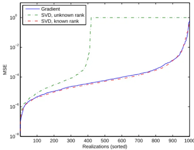
Figure 1 illustrates how the different optimization meth-ods (SVD- and gradient- based) of |C(4)z {y}| behave whenever R is not full rank (this is the case as we have chosen N = 3, Q = 5 and L = 2). The MSE on the extracted source is plotted and for readability, the 1000 realizations have been ordered by increasing value of the MSE. One can observe that the SVD-based method fails in about 60% realizations when the rank of R is unknown. On the contrary, a gradient based optimization or an SVD-based method where the rank is known yields acceptable results. Figure 2 illustrates the same phenomenon in a deflation context: the problem does not occur for the 1st source, which is coherent with our choice Q = N + 1 = 4 for which R is full rank for the first deflation step. On the contrary, the extraction of the second and third sources fails quite often.
100 200 300 400 500 600 700 800 900 1000 10−8 10−6 10−4 10−2 100 Realizations (sorted) MSE Gradient SVD, unknown rank SVD, known rank
Fig. 1. Sensitivity of the different methods to the rank of R (100000 samples, N=3, Q=5 and L=2).
0 100 200 300 400 500 600 700 800 900 1000 10−8 10−7 10−6 10−5 10−4 10−3 10−2 10−1 100 Realizations (sorted) MSE Gradient SVD, unknown rank SVD, known rank
(a) 1st extracted source
0 100 200 300 400 500 600 700 800 900 1000 10−6 10−5 10−4 10−3 10−2 10−1 100 101 Realizations (sorted) MSE Gradient SVD, unknown rank SVD, known rank (b) 2nd extracted source 0 100 200 300 400 500 600 700 800 900 1000 10−5 10−4 10−3 10−2 10−1 100 101 Realizations (sorted) MSE Gradient SVD, unknown rank SVD, known rank (c) 3rd extracted source Fig. 2. Sensitivity of the different methods to the rank of R in a deflation context (100000 samples, N=3, Q=4 and L=2).
Tables 1, 2 and 3 compare the quality result obtained for different number of samples by one gradient optimization of the two contrast functions |C(4){y}| and |C(4)
z {y}| respec-tively. We have also tried the improvement proposed in Sec-tion 5 by performing Ni = 5 maximizations of (3) and up-dating each time the reference signal. One can see that our method provides quite good results with Ni = 1 gradient optimization of |Cz(4){y}|. With Ni = 5 maximizations of |Cz(4){y}|, the MSE is as good as the result given by the kur-tosis contrast function |C(4){y}|. Finally, the execution time
is showed in Table 4: as expected, quadratic contrasts are sig-nificantly faster to maximize than kurtosis based contrast: in particular, this allows one to handle very large sample sizes.
separation method Deflation step 1st 2nd 3rd |Cz(4){y}| Ni= 1 0.0519 0.0658 0.0942 |Cz(4){y}| Ni= 5 0.0030 0.0111 0.0456 Kurtosis 0.0035 0.0087 0.0677
Table 1. Average (1000 realizations) MSE for different con-trast function and optimization methods; 1000 samples.
separation method Deflation step 1st 2nd 3rd |Cz(4){y}| Ni= 1 0.0171 0.0152 0.0339 |Cz(4){y}| Ni= 5 0.0069 0.0032 0.0174 Kurtosis 0.0028 0.0032 0.0187
Table 2. Average (1000 realizations) MSE for different con-trast function and optimization methods; 10000 samples.
7. REFERENCES
[1] M. Castella, S. Rhioui, E. Moreau, and J.-C. Pesquet. Quadratic higher-order criteria for iterative blind separation of a MIMO
separation method Deflation step 1st 2nd 3rd |C(4)z {y}| Ni= 1 0.0156 0.0114 0.0142 |C(4)z {y}| Ni= 5 0.0050 0.0027 0.0032 Kurtosis 0.0042 0.0026 0.0043
Table 3. Average (1000 realizations) MSE for different con-trast function and optimization methods; 100000 samples.
separation method Number of samples 1000 10000 100000 |Cz(4){y}| Ni= 1 1.84 2.01 4.17 |Cz(4){y}| Ni= 5 8.87 9.30 14.89 Kurtosis 9.45 49.66 578.56
Table 4. Average (1000 realizations) execution time in sec-onds for different contrast function and optimization methods. convolutive mixture of sources. IEEE Trans. Signal Processing, 55(1):218–232, January 2007.
[2] N. Delfosse and P. Loubaton. Adaptive blind separation of in-dependent sources: a deflation approach. Signal Processing, 45:59–83, 1995.
[3] D. N. Godard. Self-recovering equalization and carrier tracking in two-dimensional data communication systems. IEEE Trans. on Communications, 28(11):1867–1875, November 1980. [4] M. Kawamoto, K. Kohno, and Y. Inouye. Eigenvector
algo-rithms incorporated with reference systems for solving blind de-convolution of MIMO-IIR linear systems. IEEE Signal Process-ing Letters, 14(12):996–999, December 2007.
[5] C. Simon, P. Loubaton, and C. Jutten. Separation of a class of convolutive mixtures: a contrast function approach. Signal Processing, (81):883–887, 2001.
[6] J. K. Tugnait. Identification and deconvolution of multichan-nel linear non-gaussian processes using higher order statistics
and inverse filter criteria. IEEE Trans. Signal Processing,