Interannual variability of the Mediterranean trophic regimes from ocean color satellites

(1)

HAL Id: hal-01341963

https://hal.sorbonne-universite.fr/hal-01341963

Submitted on 5 Jul 2016

HAL is a multi-disciplinary open access

archive for the deposit and dissemination of

sci-entific research documents, whether they are

pub-lished or not. The documents may come from

teaching and research institutions in France or

abroad, or from public or private research centers.

L’archive ouverte pluridisciplinaire HAL, est

destinée au dépôt et à la diffusion de documents

scientifiques de niveau recherche, publiés ou non,

émanant des établissements d’enseignement et de

recherche français ou étrangers, des laboratoires

publics ou privés.

regimes from ocean color satellites

Nicolas Mayot, Fabrizio d’Ortenzio, Maurizio Ribera D ’Alcalà, Héloïse

Lavigne, Hervé Claustre

To cite this version:

Nicolas Mayot, Fabrizio d’Ortenzio, Maurizio Ribera D ’Alcalà, Héloïse Lavigne, Hervé Claustre.

In-terannual variability of the Mediterranean trophic regimes from ocean color satellites. Biogeosciences,

European Geosciences Union, 2016, 13 (6), pp.1901-1917. �10.5194/bg-13-1901-2016�. �hal-01341963�

(2)

www.biogeosciences.net/13/1901/2016/ doi:10.5194/bg-13-1901-2016

Interannual variability of the Mediterranean trophic regimes

from ocean color satellites

Nicolas Mayot1, Fabrizio D’Ortenzio1, Maurizio Ribera d’Alcalà2, Héloïse Lavigne3, and Hervé Claustre1

1_{Sorbonne Universités, UPMC Univ Paris 06, INSU-CNRS, Laboratoire d’Océanographie de Villefranche (LOV),}

181 Chemin du Lazaret, 06230 Villefranche-sur-mer, France

2_{Laboratorio di Oceanografia Biologica, Stazione Zoologica “A. Dohrn”, Villa Comunale, 80121 Napoli, Italy}

3_{Istituto Nazionale di Oceanografia e di Geofisica Sperimentale (OGS), Borgo Grotta Gigante 42/c,}

34010 Sgonico (Trieste), Italy

Correspondence to: Nicolas Mayot (nicolas.mayot@obs-vlfr.fr)

Received: 27 July 2015 – Published in Biogeosciences Discuss.: 9 September 2015 Revised: 10 March 2016 – Accepted: 19 March 2016 – Published: 30 March 2016

Abstract. D’Ortenzio and Ribera d’Alcalà (2009, DR09 hereafter) divided the Mediterranean Sea into “bioregions” based on the climatological seasonality (phenology) of phy-toplankton. Here we investigate the interannual variability of this bioregionalization. Using 16 years of available ocean color observations (i.e., SeaWiFS and MODIS), we analyzed the spatial distribution of the DR09 trophic regimes on an an-nual basis. Additionally, we identified new trophic regimes, exhibiting seasonal cycles of phytoplankton biomass differ-ent from the DR09 climatological description and named “Anomalous”. Overall, the classification of the Mediter-ranean phytoplankton phenology proposed by DR09 (i.e., “No Bloom”, “Intermittently”, “Bloom” and “Coastal”), is confirmed to be representative of most of the Mediterranean phytoplankton phenologies. The mean spatial distribution of these trophic regimes (i.e., bioregions) over the 16 years stud-ied is also similar to the one proposed by DR09, although some annual variations were observed at regional scale. Dis-crepancies with the DR09 study were related to interannual variability in the sub-basin forcing: winter deep convection events, frontal instabilities, inflow of Atlantic or Black Sea Waters and river run-off. The large assortment of phytoplank-ton phenologies identified in the Mediterranean Sea is thus verified at the interannual scale, further supporting the “sen-tinel” role of this basin for detecting the impact of climate changes on the pelagic environment.

1 Introduction

The Mediterranean Sea is one of the oceanic regions most impacted by climate change (Giorgi, 2006; Giorgi and Li-onello, 2008). These important environmental modifica-tions are supposed to strongly modify the dynamics of the Mediterranean marine ecosystems (The Mermex Group, 2011), by modifying the food web structure (Coll et al., 2008), triggering regime shifts (Conversi et al., 2010) or un-expected events (e.g., jellyfish blooms, Purcell, 2005), which should have strong consequences on human activities. In the context of climate change, phytoplankton plays a key role, because any perturbations on its dynamics would affect the rest of the marine food web (Edwards and Richarson, 2004). In a relatively small semi-enclosed sea, such as the Mediter-ranean, those kinds of processes should be particularly ac-celerated. A modification of the phytoplankton communities could impact the whole ecosystems much more rapidly than in other oceanic regions (Siokou-Frangou et al., 2010).

In the Mediterranean, as in many of the oceanic regions, the phytoplankton dynamics are characterized by a strong spatio-temporal variability (Estrada, 1996; Mann and Lazier, 2006), determined by the concomitant influence of several bi-otic and abibi-otic factors (Williams and Follows, 2003; Mann and Lazier, 2006). The link between abiotic factors and phy-toplankton variability, in the Mediterranean Sea, has been mainly inferred by using satellite ocean color data (Antoine et al., 1995; Bosc et al., 2004; Mélin et al., 2011; Volpe et al., 2012). Based on band-ratio algorithms that infer surface chlorophyll a concentration (considered as a proxy of

(3)

phy-toplankton biomass), a general picture of the Mediterranean was revealed, confirming and reinforcing what had been de-rived by the relatively scarce existing in situ estimations, e.g., the presence of a widespread oligotrophy, of strong east–west and north–south gradients, the coastal influences, and the oc-currence of blooming episodes in well-defined regions.

However, despite the ecological relevance of phytoplank-ton seasonality (or phenology), which provides a powerful tool to identify the factors affecting ecosystem functioning (Edwards and Richarson, 2004), phenology has received less consideration in the Mediterranean. Phytoplankton phenol-ogy was generally hard to evaluate, as observations were either not available at the required temporal and/or spa-tial resolution (see review of Ji et al., 2010), or were re-stricted to coastal areas. Satellite observations provide high-frequency temporal and spatial observations and represent the only available data set to estimate the seasonal dynam-ics of phytoplankton at basin-scale with a proper spatio-temporal resolution (Ji et al., 2010). Using satellite observa-tions, a first attempt to characterize the Mediterranean phyto-plankton phenology was recently proposed (D’Ortenzio and Ribera d’Alcalà, 2009, DR09 thereafter). Although limited to the sea surface, DR09 identified in the available SeaW-iFS ocean color data set, seven recurrent patterns in sea-sonal cycles of phytoplankton in the Mediterranean. The observed seasonal patterns (referred by DR09 as “trophic regimes”) were then regrouped in four main classes on the basis of their shape characteristics: a “temperate seas-like” dynamic (referred by DR09 as “Bloom”, characterized by a spring peak), a “tropical seas-like” dynamic (referred by DR09 as “No bloom”, to indicate the absence of a marked peak), an “intermittently” dynamic (considered as an inter-mediate regime between “Bloom” and “No Bloom” trophic regimes, and interpreted as an artifactual regime produced by averaging) and a “Coastal” dynamic (frequently observed in coastal regions, see later). Moreover, the geographical dis-tribution of the DR09 trophic regimes followed well-defined spatial patterns, and was thus interpreted as a bioregional-ization of the basin based on the phenological traits of the surface chlorophyll a concentration. Compared to other ex-isting Mediterranean bioregionalization (e.g., Nieblas et al., 2014), the DR09 approach is specifically focused on the sea-sonal cycles of phytoplankton and is consequently adapted to address issues related to phytoplankton phenology.

The DR09 results have already been used to investigate the role of the mixed layer depth (MLD) and the nitrate distribu-tion on the Mediterranean phytoplankton phenology (Lavi-gne et al., 2013), while modeling studies have used the DR09 bioregionalization based on the seasonal dynamics of phy-toplankton to ameliorate the primary production estimates from space (Uitz et al., 2012). Combining temporal (i.e., the trophic regimes) and spatial (i.e., the bioregions) analysis, the DR09 results thus provided a robust framework to iden-tify the role of abiotic and biotic factors on the Mediterranean phytoplankton phenology.

Two main issues are, however, still unresolved. Firstly, the DR09 results were obtained under a strict climatological ap-proach, providing the most relevant spatio-temporal patterns, though smoothing any interannual variability. Secondly, and as a consequence of the climatogical scale, the DR09 trophic regimes and bioregions could be an artifactual result of the climatological average, which, by flattening the seasonal cy-cle of surface chlorophyll a, could have generated unrealistic seasonal cycles of phytoplankton. This point, already evoked by the authors, is particularly relevant for the “Intermittently” trophic regime of DR09 (see also the discussion on the “In-termittently” DR09 trophic regime in Lavigne et al., 2013).

In this paper, we reappraised the DR09 approach with the specific aim to account for the interannual variability of the Mediterranean surface chlorophyll a concentration. A new method is proposed to identify the relevance of the DR09 trophic regimes on an annual basis. The method also identi-fies the discrepancy from the DR09 climatological trophic regimes, by allowing the emergence of totally new (com-pared to DR09) patterns of seasonality (i.e., new trophic regimes) that could have been masked by the climatological approach of DR09. The satellite database is also expanded, by including seven additional years of ocean color data com-pared to the DR09 paper. The discussion is focused on the interannual variability of the DR09 trophic regimes and on the occurrence of the new trophic regimes. A step forward in the interpretation of the trophic regimes is proposed (the DR09 ones and the new ones) by considering their occur-rence frequency at basin and regional scales, simultaneously with forcing processes.

2 Data and methods

2.1 Data

Surface chlorophyll a concentration ([Chl]surf) from Level

3 images of SeaWiFS and MODIS Aqua, at spatial and temporal resolution of 9 km and 8 days respectively, were downloaded from the NASA’s OceanColor website (http: //oceandata.sci.gsfc.nasa.gov/), for the period 1998–2014. SeaWiFS data were used for the period 1998–2007, while MODIS Aqua data were used after July 2007. MODIS and SeaWiFS data sets were already shown to be consistent (Franz et al., 2005). The resulting 16-year satellite database was initially divided on a yearly basis (from July of year T −1 to late June of year T ) and a 3-week (i.e., 24 days) moving average was applied. In the Mediterranean Sea, an

overesti-mation of the [Chl]surfretrieved from space was identified by

comparison with in situ data (Gitelson et al., 1996; Claus-tre et al., 2002), particularly at the low values (e.g., Fig. 14 from Antoine et al., 2008). However, to be consistent with the DR09 analysis, the NASA standard products for SeaW-iFS and MODIS (O’Reilly et al., 1998) were used here, in-stead of alternative products generated through regional

(4)

algo-Figure 1. Schematic representation of the different steps of the method used in this study (see Sect. 2.2 for details).

rithms. Consequently, as in DR09, to minimize the impact of

the [Chl]surfalgorithms artifacts and in order to focus on the

seasonal variations of the [Chl]surf(regardless of the existing

difference between the Mediterranean Sea areas in the values

of [Chl]surf), each annual time series was normalized by its

maximal value. In what follows, the time series (from July to June) of a specific year are referred to as “annual” time series of normalized surface chlorophyll a concentration (nChl).

2.2 Interannual clustering

The method proposed here initially uses the trophic regimes identified by DR09 to classify pixels on an annual basis. The method consists in identifying, for each “annual” time se-ries of each pixel, the DR09 trophic regime with the most similar time series. After this first classification, a number of time series remain unclassified (i.e., “non assigned”). These “non assigned” time series are then clustered to identify new

(5)

trophic regimes, which were somehow hidden in the DR09 approach.

In practice (see Fig. 1):

1. For each year and for each Mediterranean pixel, the “an-nual” time series of nChl and its corresponding geo-graphical position are extracted (Fig. 1, step 1). 2. The similarity between the “annual” time series and

each of DR09 trophic regimes is evaluated using the Chebyshev distance (e.g., Han et al., 2011), with only the 8-day averages of nChl as variables (i.e., 46

vari-ables). Between two time series X = (x1, x2. . .xn)and

Y = (y1, y2. . .yn)the Chebyshev distance (dXY)is

de-fined as dXY = lim p→∞ n X i=1 |xi−yi|p !1_p =maxn i=1|xi −yi| , (1)

with n = 46. The DR09 trophic regime having the low-est Chebyshev distance with the “annual” time series is initially selected (Fig. 1, step 2).

3. To be definitively assigned to the selected DR09 trophic regime, the “annual” time series must be contained in the confidence interval of that DR09 trophic regime. The confidence interval is defined as the mean Cheby-shev distance between the DR09 trophic regime and all the weekly climatological time series of nChl used by DR09 that belong to this trophic regime, plus 1.5 times the standard deviation (Fig. 1, step 3). Note that the confidence interval is different for each DR09 trophic regime.

4. If the “annual” time series falls within the confidence interval, then the “annual” time series and its pixel are assigned to the DR09 trophic regime initially selected (Fig. 1, step 4). Otherwise, the “annual” time series (and its associated pixel) is temporarily added to a table with all “non-assigned” time series. At this stage, 16 annual maps (not shown) were obtained, indicating if the times series of each pixel were still “non assigned”, or other-wise the membership of the pixels as one of the DR09 trophic regimes.

5. All of the “non-assigned” time series (from all the 16 years combined) were clustered by using a K-means clustering (Hartigan and Wong, 1979; Fig. 1, step 5). The number of clusters is decided using the Calinski and Harabasz index (this index compared the within and between cluster variance, Calinski and Harabasz, 1974; Milligan and Cooper, 1985). Then, the stability of the resulting clusters was assessed by comparing them (using the Jaccard coefficient) with clustering results obtained after a modification (i.e., adding an artificial noise), or a subset of the data set (Hennig, 2007, see also

DR09). Only clusters with a Jaccard coefficient greater than 0.75 are considered stable. These new clusters in-clude all the “annual” time series that are statistically different from the DR09 climatological time series. In some sense, they represent anomalies compared to the DR09 climatological analysis and, for this reason, they are referred in the following as “Anomalous” trophic regimes.

Four “Anomalous” trophic regimes are obtained, and all are stable (i.e., presenting Jaccard coefficients > 89 %). Overall, 77.2 % of the “annual” time series is classified as one of the DR09 trophic regimes, and 12.8 % as one of the “Anoma-lous” trophic regimes.

3 Results

The method described in Sect. 2.2 provides 11 time series (i.e., the seven DR09 trophic regimes and the four “Anoma-lous”) obtained by averaging all the “annual” time series of

nChl based on their membership in one of the 11 trophic

regimes (Fig. 2), as well as 16 annual maps of the spatial distribution of the 11 trophic regimes (Fig. 3). Following the interpretation of DR09, we considered the spatial distribu-tion of the trophic regimes as a bioregionalizadistribu-tion, and we will refer the regions having the same trophic regime as a “bioregion”.

The main traits of the trophic regime time series is sketched in the next paragraphs (for the seven DR09 and the four “Anomalous”), whereas their associated geograph-ical distributions is analyzed afterwards.

3.1 General patterns of DR09 trophic regimes

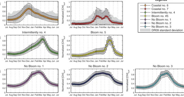
The nChl time series of the non-coastal DR09 trophic regimes (Fig. 2), in spite of their common characteristics (they all present minimal value in summer, Table 1),

dis-play different amplitudes of nChl and [Chl]surf(i.e., defined

as the difference between the mean summer value and the

annual maximum values of nChl and [Chl]surf, Table 1).

The “Bloom #5” and “Intermittently #4” trophic regimes

show the greatest amplitudes (0.66 nChl and 0.82 mg m−3

for “Bloom #5”, 0.63 nChl and 0.40 mg m−3for the

“Inter-mittently #4”), whereas the “No Bloom #2” trophic regime

the lowest (0.48 nChl and 0.14 mg m−3₎_{. The timings of}

the main events are also different. The dates of the annual maximum values are observed in winter (February) for “No Bloom” trophic regimes (#1, #2 and #3) and in spring for the “Intermittently #4” (March) and the “Bloom #5” (April) trophic regimes. The dates of the maximal rate of change (i.e., the date of the highest first derivative of the nChl time series) are increasing from the “No Bloom”, the “Intermit-tently #4”, to the “Bloom #5”, whereas the dates of the min-imum rate of change (i.e., the date of the lowest first

(6)

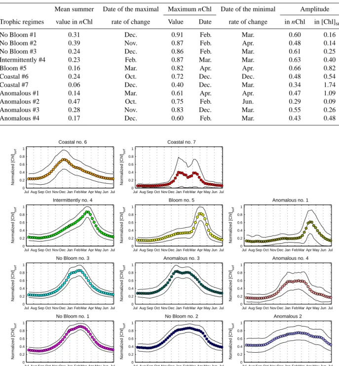
deriva-Table 1. Index on the trophic regimes’ mean time series (Fig. 2). Summer is defined from June to August, and the date of the maximal

and/or minimal rate of change as the date of the highest and/or lowest first derivative of the mean time series of nChl. Whereas the amplitude corresponds to the difference between the mean summer values and the annual maximum values of nChl or [Chl]surf(see Sect. 3.2).

Mean summer Date of the maximal Maximum nChl Date of the minimal Amplitude Trophic regimes value in nChl rate of change Value Date rate of change in nChl in [Chl]surf

No Bloom #1 0.31 Dec. 0.91 Feb. Mar. 0.60 0.16 No Bloom #2 0.39 Nov. 0.87 Feb. Apr. 0.48 0.14 No Bloom #3 0.24 Dec. 0.86 Feb. Mar. 0.61 0.25 Intermittently #4 0.23 Feb. 0.87 Mar. Mar. 0.63 0.40

Bloom #5 0.16 Mar. 0.82 Apr. Apr. 0.66 0.82

Coastal #6 0.24 Oct. 0.72 Dec. Dec. 0.48 0.54

Coastal #7 0.06 Dec. 0.40 Dec. Mar. 0.34 1.74

Anomalous #1 0.14 Mar. 0.61 Apr. Apr. 0.47 1.09 Anomalous #2 0.47 Oct. 0.75 Feb. Jun. 0.29 0.09 Anomalous #3 0.28 Nov. 0.83 Dec. Mar. 0.55 0.26 Anomalous #4 0.17 Dec. 0.60 Feb. Mar. 0.43 0.48

Jul Aug Sep Oct Nov Dec Jan Feb Mar Apr May Jun Jul 0 0.2 0.4 0.6 0.8 1 Normalized [Chl] su rf Coastal no. 6

Jul Aug Sep Oct Nov Dec Jan Feb Mar Apr May Jun Jul 0 0.2 0.4 0.6 0.8 1 Normalized [Chl] su rf Coastal no. 7

Jul Aug Sep Oct Nov Dec Jan Feb Mar Apr May Jun Jul 0 0.2 0.4 0.6 0.8 1 Normalized [Chl] su rf Intermittently no. 4

Jul Aug Sep Oct Nov Dec Jan Feb Mar Apr May Jun Jul 0 0.2 0.4 0.6 0.8 1 Normalized [Chl] su rf Bloom no. 5

Jul Aug Sep Oct Nov Dec Jan Feb Mar Apr May Jun Jul 0 0.2 0.4 0.6 0.8 1 Normalized [Chl] su rf Anomalous no. 1

Jul Aug Sep Oct Nov Dec Jan Feb Mar Apr May Jun Jul 0 0.2 0.4 0.6 0.8 1 Normalized [Chl] su rf No Bloom no. 3

Jul Aug Sep Oct Nov Dec Jan Feb Mar Apr May Jun Jul 0 0.2 0.4 0.6 0.8 1 Normalized [Chl] su rf Anomalous 2

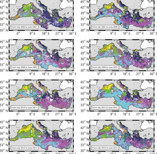
Figure 2. Mean time series of the seven DR09 trophic regimes (“No Bloom #1”, “No Bloom #2”, “No Bloom #3”, “Intermittently #4”,

“Bloom #5”, “Coastal #6” and “Coastal #7”) and of the four “Anomalous” trophic regimes (“Anomalous” #1, #2, #3 and #4) obtained from our method. Standard deviations are indicated as black lines.

tive of the nChl time series, the most negative value) range between March (“No Bloom #3”) and April (“Bloom #5).

The “Coastal” DR09 trophic regimes show different sea-sonal characteristics from the rest of the DR09 trophic regimes (Table 1). The maximum value of the “Coastal #6”

time series is lower (0.72 nChl) and arrives earlier (Decem-ber) than for the other DR09 trophic regimes. The “Coastal #7”, which shows a double peak during winter months, ex-hibits also a great dispersion around the mean, indicating that the resulting mean seasonal cycle is probably an artifact.

(7)

Figure 3.

3.2 General patterns of the “Anomalous” trophic regimes

All of the “Anomalous” trophic regimes (#1, #2, #3 and #4) show minimum values of nChl in summer (0.14 nChl for the “Anomalous #1”, 0.47 nChl for the “Anomalous #2”, 0.28

nChl for the “Anomalous #3 and 0.17 nChl for the

“Anoma-lous #4”). The “Anoma“Anoma-lous #1” trophic regime shows an evident spring peak (starting in March, maximal in early April and decreasing in mid-April), whereas “Anomalous #2”, “#3” and “#4” display a winter plateau, with their max-imal rate of change and maxmax-imal values obtained in late fall and winter respectively (in October and February for “#2”,

(8)

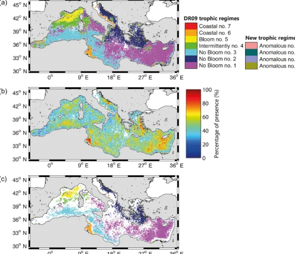
Figure 3. Maps of the spatial distribution of the trophic regimes (i.e., bioregions), (a) for the years 1999 to 2006 and (b) for the years 2007 to

2014. Note that the year is defined from July to June, (example for the map 1999, it corresponds to the period from July 1998 to June 1999). The white pixels indicate “no data”.

in November and December for “#3” and in December and February for “#4”).

All the above suggests that the “Anomalous” trophic regimes could be considered as modified versions of the DR09 trophic regimes. The “Bloom #5” and the “Anomalous #1” trophic regimes have a similar shape, showing both a spring peak (for both the date of the maximal value in April). Although they differ slightly for the dates of the maximal and minimal rate of change (early March and late April for “Bloom #5”, and late March and mid-April for the “Anoma-lous #1”), the “Anoma“Anoma-lous #1” trophic regime appears as a more peaked version of the “Bloom #5” trophic regime, with

a higher amplitude in [Chl]surf(0.82 mg m−3for the “Bloom

#5” and 1.09 mg m−3for the “Anomalous #1”).

Similarly, the “No Bloom #2” and the “Anomalous #2” trophic regimes could be associated. They both

dis-play weak amplitudes of nChl and of [Chl]surf (0.48 nChl

and 0.14 mg m−3 _{for the “No Bloom #2”, 0.29 nChl and}

0.09 mg m−3_{for the “Anomalous #2”, which are among the}

lowest of the non-coastal trophic regimes). They mainly dif-fer in the date of the minimal rate of change, which is delayed for 2 months for the “Anomalous #2” (in June) compared to the “No Bloom #2” (in April). The “Anomalous #2” trophic regime appears as a smoothed version of the “No Bloom

(9)

Figure 4. (a) Time series of the area cover by the different

biore-gions each year (in % of the Mediterranean classified). All “No Bloom” bioregions are regrouped together, as well as all “Coastal” and all “Anomalous” bioregions. (b) Same as Fig. 4a but only for the three “No Bloom” bioregions.

#2” trophic regime, where the winter-to-summer difference is low.

Finally, the “No Bloom #3” and the “Anomalous #3” and “#4” trophic regimes have similar shapes and spatial repar-tition (see the next section). However, the “Anomalous #3” trophic regime displays differences in the timing of the max-imal rate of change and of the maxmax-imal value (in Novem-ber and DecemNovem-ber for the “Anomalous #3”, and in Decem-ber and February for the “No Bloom #3”), and the “Anoma-lous #4” trophic regime presents a higher maximal value

of [Chl]surf(0.68 mg m−3)than the “No Bloom #3” trophic

regime (0.35 mg m−3), but a lower maximal value of nChl

(0.60 nChl for the “Anomalous #4” and 0.86 nChl for the “No Bloom #3”), indicating a variability in the timing of the peak between individual time series.

The association of the “Anomalous” trophic regimes with the DR09 trophic regimes confirms the general partitions proposed by DR09 into “Bloom” and “No Bloom” trophic regimes. The low occurrence of the “Anomalous” trophic regimes indicates also that their importance in the basin be-havior is low. They possibly signify an accentuation or a di-minishing of the factors influencing the phytoplankton phe-nology, although they should be likely considered as tem-porary perturbations of the general “Bloom”/”No Bloom” regimes. We will discuss this later.

3.3 Geographical distribution of trophic regimes: interannual variability

The 16 annual maps, showing the spatial distribution of the 11 trophic regimes (Fig. 3), represent a first attempt to eval-uate the interannual spatial variability of the bioregions

(de-fined, in the sense of DR09, as regions having similar phy-toplankton phenology or, more precisely, having the same trophic regime). In the next, the results are presented fol-lowing the four main DR09 groups of trophic regimes (i.e., “No Bloom”, “Bloom”, “Intermittently” and “Coastal”). The “Anomalous” trophic regimes are discussed separately. The last paragraph will be dedicated to a wider analysis on the interannual spatio-temporal variability of the bioregions.

3.3.1 The “No Bloom” trophic regimes

Over the studied 16 years, “No Bloom” bioregions cover most of the Mediterranean Sea (67.2 % on average, Fig. 4). The “No Bloom #1” is the most occurring “No Bloom” biore-gion (Fig. 4). Exceptions are observed in 1999, 2001, 2004, 2012 (dominance of the “No Bloom #3”) and in 2000, 2007 (dominance of the “No Bloom #2”). The “No Bloom #1” bioregion is permanently observed in the Levantine basin, and often in the Ionian Sea (Fig. 3). Episodically, it is also ob-served in the western basin, in particular over the Tyrrhenian Sea. During the 1999 to 2007 period, the “No Bloom #1” bioregion on average covered 25.6 % of the Mediterranean Sea, while from 2008 to 2014, its mean percentage increases to 33.5 %.

The second most occurring bioregion is the “No Bloom #3”, with a mean value of 21.5 % of covered surface over the 16 years (Fig. 4). It is associated with the Algerian basin (except in 2013 and 2014), although its northern and eastern boundaries are more variable (Fig. 3). It is also observed in the Northwestern Mediterranean (NWM), in the Tyrrhenian, and sometimes in a large portion of the eastern basin (i.e., 2004 and 2012). No clear trends are observed over its inter-annual evolution, except in 1999, 2001, 2004 and 2012, when it was the most widespread bioregion.

Finally, the “No Bloom #2” bioregion covers 16.7 % of the Mediterranean Sea on average (Fig. 4), and it is permanently observed in the Aegean and Adriatic Seas (Fig. 3). Peaks of occurrence are observed in 2000 and 2007, when its distri-bution extended over the North Ionian (in 2000) and most of the eastern Basin (in 2007). Similarly to the “No Bloom #1” bioregion, two periods could be identified in its interan-nual trend. Before 2008, the occurrence of the “No Bloom #2” bioregion is erratic, ranging from 11.5 to 31.7 %. After 2008, the surface cover is low (i.e., 10.4 % on average) and constant.

3.3.2 The “Bloom” trophic regime

The “Bloom #5” bioregion covers 4 % of the Mediterranean Sea on average (Fig. 4), and it is observed quite exclusively in the NWM (Fig. 3). Notable exceptions are the years 1999 and 2006, when it is observed in the Southern Adriatic, and in 2003, in the Rhodes gyre area. The interannual variabil-ity of its extent (Fig. 4) ranges from very low values (i.e., in 2001, 2007 and 2014) up to 9 % of the total Mediterranean

(10)

surface (i.e., in 2005, which is, however, a special year due to a high number of missing values). When the “Bloom #5” bioregion is weakly observed, it is generally replaced either by “Intermittently #4” (i.e., as in 2001 or in the 2007) or by the “Anomalous #1” bioregion (Fig. 3). In the first case, the “Intermittently #4” bioregion extends all over the NWM with an almost total disappearance of the “Bloom #5” biore-gion. In the second case, the “Bloom #5” bioregion is still present, but located in the border area of the NWM. Instead, the central area is occupied by the “Anomalous #1” bioregion (especially in 2005, 2006, 2008, 2010, 2013 and 2014).

3.3.3 The “Intermittently” trophic regime

On average, the “Intermittently #4” bioregion occupies 12.2 % of the Mediterranean Sea (Fig. 4). However, this per-centage shows strong interannual variations, ranging from 7.2 to almost 24.5 % of the total surface. It is permanently observed in the NWM, in the frontal area south of the large cyclonic gyre of the Ligurian Sea (Fig. 3). Its interannual variability is expressed by the high values of occurrence in 2003, 2006, 2007 and 2013, for the most part in the western basin. In the eastern basin, it is recurrently observed in the Rhodes Gyres (2000, 2003, 2005, 2006, 2007, 2008, 2009 and 2012), in the North Ionian (1999, 2000, 2006, 2008 and 2012) and in the Southern Adriatic (1999, 2002, 2007, 2008, 2012 and 2014).

3.3.4 The “Coastal” trophic regimes

The “Coastal” bioregions cover 3.5 % of the Mediterranean Sea on average (Fig. 4), with a weak interannual vari-ability (±1.5 %). The varivari-ability of the “Coastal” biore-gions is mainly driven by the variation of the occurrence of the “Coastal #6” bioregion, which represents 95 % of the “Coastal” bioregions occurrence. It is permanently observed in the Gulf of Gabes and, more sporadically, in the west Adri-atic coast (in 2002, 2003 and 2011, Fig. 3).

The “Coastal #7” bioregion, being rarely present, (less than 0.25 % of the Mediterranean Sea), will be neglected in the rest of the present study.

3.3.5 The “Anomalous” trophic regimes

The “Anomalous” bioregions occupy 12.8 % of the sur-face basin on average (Fig. 4), although they are primarily concentrated in coastal zones: the “Anomalous #2” biore-gion along the Adriatic and Aegean coasts, the “Anomalous #3” bioregion along the southeastern basin coasts and the “Anomalous #4” bioregion along the Algerian coast (Fig. 3). Apart from coastal zones, the “Anomalous #1” bioregion is episodically observed in the NWM, where it occupies a re-gion usually classified as “Bloom #5” (see Sect. 3.3.2).

3.3.6 Dominance maps

Although interannual variability in the geographical distribu-tion of the bioregions is high, some general patterns emerge. To demonstrate this, a dominance map was calculated by evaluating, for each pixel, the most recurrent bioregion (i.e., the dominant regime), over the 16-year period (Fig. 5a). Most of the Mediterranean basin is assigned to one of the DR09 bioregions (96 % of the map) and only 4 % to an “Anoma-lous” bioregion. A second map showing the degree of mem-bership (defined as the percent of years in which each pixel belongs to its most recurrent bioregion, Fig. 5b) was gen-erated. The mean degree of membership over the whole Mediterranean area is 46 % (Fig. 5b), quantifying the large interannual variability of the basin. Spatial differences are, however, visible: coastal zones are generally characterized by a low degree of memberships, while open-ocean regions display higher values, showing less interannual variability.

To better highlight these geographical patterns, only areas with a degree of membership greater than 50 % were plot-ted (Fig. 5c). The colored areas in Fig. 5c indicate where the bioregions are the most temporally recurrent, reflecting then the regions characterized by a weak interannual variability in the phenological traits. All the coastal areas (except in the Gulf of Gabes), as well as the regions at the frontier between bioregions, disappear. Most of the “Intermittently #4” biore-gion also disappear (maintained only in a limited rebiore-gion of the NWM), as well as all the “Anomalous” bioregions (ex-cept the “Anomalous #1” bioregion in the NWM) and most of the region of the Alboran Sea.

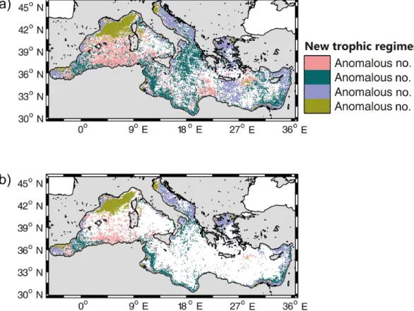
Similarly, a dominance map generated by considering the four “Anomalous” bioregions only (Fig. 6a), shows their patchy distribution and irregular occurrences. How-ever, some spatial patterns exist, and are highlighted when only the pixels having at least two occurrences of the same “Anomalous” bioregion over the 16-year period were shown (Fig. 6b). The Anomalous #2, #3 and #4 bioregions are re-currently observed, but only along coasts. As always high-lighted, the only open-ocean region exhibiting a coherent and recurrent “Anomalous” pattern is the NWM (classified as “Anomalous #1”).

4 Discussion

4.1 Comparison with DR09 classification

The new method proposed here is intrinsically different from the one of DR09, although it similarly provides trophic regimes and their spatial distributions (interpreted here as bioregions). A comparison between the two approaches is therefore required before discussing the results.

To do so, we verified that the algorithms used in the new method provide the same results as the DR09 methodology (i.e., generation of a weekly climatological database and then

(11)

Figure 5. (a) Map of the most recurrent bioregions for the 16-year period (i.e., the dominant regimes), obtained with our method. The white

pixels indicate where data are mostly not available. (b) Map of the percentage of presence of the dominant regimes. (c) Map of the most recurrent bioregions as in Fig. 5a, but displaying only pixels with a percentage of presence ≥ 50 %.

application of a K-means clustering) when the results are pre-sented in a climatological point of view (i.e., on average over the 16 years). Then, all the “annual” time series of nChl were averaged according to the DR09 trophic regimes to which they belong (i.e., the DR09 trophic regimes time series in Fig. 2), and compared to the DR09 evaluations (Fig. 7). The time series obtained with the new method are equivalent to the estimations of DR09: they are contained in the confidence interval and they show similar standard deviations. The only notable discrepancy is observed for the “Coastal #7” trophic regime. Our interpretation is that the seasonal signal of this trophic regime (as obtained by DR09) is too ambiguous (i.e., high standard deviation, signal relatively flat) to be retrieved with the new method used here.

Furthermore, the spatial distribution of trophic regimes obtained with the DR09 methodology (Fig. 8) applied on the new 16-year database, is close to the dominance map of Fig. 5a (74 % of similarity, defined as the percentage of pix-els in Fig. 5a belonging to the same DR09 trophic regime in Fig. 8). However, some differences with the DR09 10-year

map (see Fig. 4 of DR09) exist, mainly the disappearance of the “Intermittently #4” bioregion in the North Ionian. The differences observed when using the new method could be ascribed more to the natural interannual variability, rather than to biases introduced through the novel methodology. Note also that the observed differences with the DR09 10-year map could additionally be ascribed to the 7-10-year exten-sion of the database. In concluexten-sion, the new method proposed here broadly supports the results of DR09 obtained at the climatological timescale, but there are some key differences generated by the larger extension of the database, or by the intrinsic natural interannual variability of the Mediterranean. We will address this last point in the next section.

4.2 Interannual spatial variability of trophic regimes: significance and forcing factors

Fig. 5c clearly indicates that the interannual variability is mostly part concentrated at the boundaries between biore-gions. In addition, the four “Anomalous” trophic regimes, although statistically significant (i.e., Jaccard coefficient

(12)

Figure 6. (a) Map of the most recurrent bioregions, calculated only for the “Anomalous” bioregions. (b) As in the Fig. 6a, but only the pixels

that had at least their most recurrent bioregion for 2 years are represented.

> 89 %), have recurrent patterns in open-ocean only in the NWM (Fig. 6b). In the rest of the basin, they appear more as episodic fluctuations or noise than as real patterns. Al-though not surprising given the approach used (i.e., first find-ing occurrence of the DR09 trophic regimes and only second searching for anomalies), this point is not trivial. From the methodological point of view, the capability of the method to detect four anomalies demonstrates its potential application in long-term studies. However, at a more in-depth analysis and in view of an oceanographic interpretation, these anoma-lies are not particularly relevant, as occurring only episodi-cally and rarely indicating coherent, recurring patterns. Thus, the main climatological bioregions identified by DR09 (i.e., “No Bloom”, “Bloom”, “Intermittently” and “Coastal”) are sufficiently comprehensive to summarize the surface phyto-plankton phenology in the Mediterranean Sea, even at inter-annual level. A notable exception in this global picture is the NWM area, with the recurrent occurrence of the “Anomalous #1” trophic regime.

Finally, it is important to note that, as suggested by DR09, each bioregion (even the “Anomalous” bioregions) is directly

related to a specific range of [Chl]surf (see Table 1). This

point suggests that the shape of the nChl time series could be related to the annual stock of phytoplankton biomass that the system could support. Based on the analysis of satellite

surface data, this observation is certainly partial, although in-dicating a real pattern that merits further investigations.

4.2.1 The “No Bloom” trophic regimes

The unimodal pattern of “No Bloom” regimes, with a higher biomass in fall-winter and lower biomass in spring–summer, were explained in DR09 by a combined mechanism involv-ing both the vertical redistribution of biomass in fall–winter (i.e., at the deepening of MLD) and the seasonality in the ra-tio consumers vs. primary producers. More recently, Lavigne et al. (2013) demonstrated the absence of light limitation in the “No Bloom” areas, confirming that the winter increase of

[Chl]surf is likely related to relatively small nutrient inputs,

as a consequence of MLD deepening. However, in winter the daily photosynthetically available radiation (PAR) at sea sur-face is also reduced. In response, the intracellular chlorophyll content in the phytoplankton cells increase (i.e., photoaccli-matation process), which increases the ratio of chlorophyll to carbon biomass (e.g., Behrenfeld et al., 2005), and could in part contribute to the temporal variations of the nChl ob-served in these “No Bloom” bioregions.

Among the three “No Bloom” trophic regimes, how-ever, and considering their geographical distribution, the “No Bloom #3” bioregion was interpreted by DR09 as driven by

(13)

Jul Aug Sep Oct Nov Dec Jan Feb Mar Apr May Jun Jul 0 0.2 0.4 0.6 0.8 1 Normalized [Chl] sur f Coastal no. 6

Jul Aug Sep Oct Nov Dec Jan Feb Mar Apr May Jun Jul 0 0.2 0.4 0.6 0.8 1 Normalized [Chl] sur f Coastal no. 7

Jul Aug Sep Oct Nov Dec Jan Feb Mar Apr May Jun Jul 0 0.2 0.4 0.6 0.8 1 Normalized [Chl] su rf Intermittently no. 4

Jul Aug Sep Oct Nov Dec Jan Feb Mar Apr May Jun Jul 0 0.2 0.4 0.6 0.8 1 Normalized [Chl] su rf Bloom no. 5

Jul Aug Sep Oct Nov Dec Jan Feb Mar Apr May Jun Jul 0 0.2 0.4 0.6 0.8 1 Normalized [Chl] sur f No Bloom no. 1

Jul Aug Sep Oct Nov Dec Jan Feb Mar Apr May Jun Jul 0 0.2 0.4 0.6 0.8 1 Normalized [Chl] sur f No Bloom no. 2

Jul Aug Sep Oct Nov Dec Jan Feb Mar Apr May Jun Jul 0 0.2 0.4 0.6 0.8 1 Normalized [Chl] sur f No Bloom no., 3 Coastal no. 6 Coastal no. 7 Intermittently no. 4 Bloom no. #5 No Bloom no. 1 No Bloom no. 2 No Bloom no. 3 DR09 standard deviation Legends

Figure 7. Mean time series of the DR09 trophic regimes (in color) and their standard deviations (vertical bars) obtained from our analysis.

The standard deviations from the DR09 methodology (in shade area) are obtained by applying the DR09 methodology (i.e., a K-means) on a weekly climatology done with the 16-year database.

Figure 8. Spatial distribution of the climatological trophic regimes obtained from the DR09 methodology (i.e., a K-means) applied on a

weekly climatology calculated from the 16-year database.

the Atlantic Water inflow from Gibraltar. The interannual variability of the Gibraltar water inflow was recently assessed (Boutov et al., 2014; Fenoglio-Marc et al., 2013), by com-bining in situ observations, modeling experiments and atmo-spheric estimations. Inflow at Gibraltar over the 1999–2008 period was maximum in 2001 and minimum in 2002, 2005 and 2007, whereas it was constant around its mean value dur-ing the other years (Boutov et al., 2014). The occurrence of the “No Bloom #3” bioregion, calculated exclusively over the Western Mediterranean (as in Fig. 4, not shown), follows a similar behavior, with an absolute maximum in 2001 and two relative minima in 2002 and 2007 (the lack of data pre-vents an evaluation of the “No Bloom #3” bioregion occur-rence in 2005). The interannual occuroccur-rence of the “No Bloom #3” bioregion appears related to the Gibraltar water inflow.

Although speculative, this correlation seems to confirm the predominant role of the Atlantic Water in shaping interan-nual variability of phytoplankton phenology in this region. Interestingly, the “Anomalous #4” trophic regime, already identified as a slightly modified version of the “No Bloom #3” trophic regime, is observed mainly in the Algerian Basin (see Fig. 6). It could indicate the presence and/or absence of episodic anticyclonic eddies (see Olita et al., 2011), gen-erated by instabilities of the Algerian current (Millot et al., 1990), which could induce slight variations of the annual phenology by locally modifying the surface layers.

The geographical distribution of the other two “No Bloom” trophic regimes (#1 and #2) is rather stable, with a predominance of the #2 in the Adriatic, Aegean and North Ionian and of the #1 in the Tyrrhenian, Levantine and

(14)

South-ern Ionian (Fig. 5a). However, in the WestSouth-ern Adriatic and in the Northern Aegean seas, which are linked to the “No Bloom #2” bioregion, an important interannual variability is observed (Fig. 5c). In the Adriatic, the organic and inorganic matter run-off generated by rivers in the Italian and Balkan peninsulas is characterized by important interannual variabil-ity, which is generally related to the timing and the intensity of the run-off. This interannual variability, which controls the injection of river nutrients into oceanic surface waters (Rev-elante and Gilmartin, 1976; Aubry et al., 2012), could induce the phenological changes observed in the North Adriatic. In the North Aegean Sea, the influence of the rivers and of the Black Sea Water on the phytoplankton productivity has been recently confirmed (Tsiaras et al., 2012, 2014; Petihakis et al., 2014). The load of nutrients in these areas by the river and/or the Black Sea Water in late spring (in May, Balkis, 2009) could also explain the occurrence of the “Anomalous #2” trophic regime, which presents a “plateau” in May, in-stead of the “No Bloom #2” trophic regime. At an interannual level, however, no trends or correlations have been identified. The rest of the spatial modifications concerning both the “No Bloom #1” and the “No Bloom #2” bioregions are for the most part induced by the eastward extension of the “No Bloom #3” or by the appearance of the “Bloom #5” and/or “Intermittently #4” bioregions. The first case is likely related to the spreading of Atlantic Water, as already mentioned. The second case, discussed in the next section, could be ascribed to local sub-basin forcing, which enables favorable blooming conditions in specific years.

4.2.2 The “Bloom” trophic regime

In the DR09 climatological classification, only one trophic regime exhibited a clear spring peak, and was therefore named “Bloom #5”. Located exclusively in the NWM, the most productive area in the Mediterranean Sea (Morel and André, 1991; Bosc et al., 2004), it was associated with the winter deep convection (MEDOC Group, 1970; Marshall and Schott, 1999; D’Ortenzio et al., 2005; Schott et al., 1997), which induces a large phytoplankton bloom through intense nutrient uptake (Marty et al., 2002). An important interan-nual variability on the intensity of the winter deep convec-tion has been observed, for the most part related to the vari-ability of atmospheric and hydrodynamic forcing (Mertens and Schott, 1998; L’Hévéder et al., 2013). In response to this oceanic and atmospheric variability, significant interan-nual differences in the biological response were also reported (Marty et al., 2002; Herrmann et al., 2013; Severin et al., 2014).

Our 16-year analysis confirms the recurrent presence of the “Bloom #5” bioregion in the NWM area, although it also highlights the sporadic occurrence of the “Anomalous #1” trophic regime, considered as a modified version of the “Bloom #5” bioregion (more peaked than the “Bloom #5” regime, see Sect. 3.2). The occurrence of the “Anomalous

#1” regime in the NWM temporally coincides with recorded events of exceptionally deep winter convection in the area (years 2005, 2006, 2008, 2010 and 2013; Smith et al., 2008; Bernardello et al., 2012; Herrmann et al., 2010; Houpert et al., 2014). Such temporal coincidence suggests that deep convection events could impact the phytoplankton phenology of the region, by inducing a stronger phytoplankton bloom

(i.e., a higher amplitude, 0.82 mg m−3 for the “Bloom #5”

trophic regime and 1.09 mg m−3 for the “Anomalous #1”

trophic regime) and a delay of the spring peak of a few weeks. This stronger NWM spring bloom induced by the in-tense deep convection events could be the result of either an increased nutrient concentration, or a modified nutrient stoi-chiometry, and/or of an enhanced zooplankton dilution, all these mechanisms being triggered by the deep convection (Herrmann et al., 2013; Severin et al., 2014). In summary, the presence of the “Anomalous #1” bioregion appears as a clear indicator of the phenological and ecological changes induced by deep convection events.

On the other hand, the recurrent occurrence of the “Bloom #5” regime in the NWM area suggests that important phy-toplankton growth occurs also when deep convection is rel-atively weak (as in 2001 and 2007, Houpert et al., 2014). However recent results from profiling floats measuring the [Chl] and the particle mass concentration, suggest also that in this region the photoacclimatation process could contribute

to the change in the [Chl]surfobserved (up to 70 %, Mignot

et al., 2014). Other recent results from profiling floats mea-suring nitrate concentration (D’Ortenzio et al., 2014) suggest that, more than the deep convection events, the permanent cy-clonic circulation in this region was the primary factor induc-ing favorable conditions for phytoplankton bloom, by brinduc-ing- bring-ing the nitracline depths close to surface. This uplift of the nitracline by the cyclonic circulation should allow an effi-cient replenishment of nitrate in surface, and the appearance of the “Bloom #5” bioregion even during mild winters. As a matter of fact, the area is never classified as a “No Bloom” bioregion.

Unlike DR09, the “Bloom #5” regime is also observed in the Southern Adriatic, in the Rhodes Gyres area and in the central Tyrrhenian. In the DR09 climatological analysis, these regions were all classified as “Intermittently #4”, and they are discussed in the next section.

4.2.3 “Intermittently #4” trophic regime

The “Intermittently” trophic regime was explained by DR09 as an effect of the interannual alternation of the “Bloom” and “No Bloom” conditions. Therefore, the resulting regime should be an artifact of the climatological approach of DR09. More recently, the interannual switch between the “Bloom” and “No Bloom” regimes over the “Intermittently #4” area was partially confirmed using in situ estimations of the MLD, although the number of observations was too scarce to draw any conclusions at the basin scale (Lavigne et al., 2013).

(15)

Here, the interannual analysis over the 16-year period indi-cates that, among the regions classed as “Intermittently #4” by DR09, the Balearic front is permanently classified as “In-termittently #4” (Fig. 5c), while the Rhodes Gyre and the Adriatic and North Ionian seas switch between “Bloom”, “No Bloom” and “Intermittently” bioregions. In other words, the DR09 “Intermittently #4” regime is confirmed to be strongly impacted by the interannual variability. However, its permanent occurrence in the Balearic Sea and its spo-radic presence in the rest of the basin suggest that it could be considered a “true” regime more than an artifact of the aver-age. The “Intermittently #4” trophic regime should be con-sidered truly an intermediate regime between “No Bloom” and “Bloom” trophic regimes. Thus the name “Intermittently #4” will be replaced by “Intermediate #4”.

Its occurrence in the Balearic area could be then ascribed to frontal instabilities that are generated all along the Balearic front (Lévy et al., 2008; Taylor and Ferrari, 2011) dur-ing the bloomdur-ing period (Olita et al., 2014). These insta-bilities (i.e., eddies, gyres or filaments) could also modify the local distribution of surface phytoplankton, by exporting phytoplankton-rich waters in the oligotrophic waters south of the Balearic front and vice versa. The chaotic nature of these instabilities could explain the lack of clear trends in the “Intermediate #4” (before considered as “Intermittently #4”) spatial variability.

For the Southern Adriatic, similar to the NWM, the cy-clonic circulation and the atmospheric conditions are gener-ally evoked to explain the bloom onset, as the deep mixing recurrently observed in the area is supposed to inject enough nutrients to sustain phytoplankton growth (Gacic et al., 2002; Civitarese et al., 2010; Shabrang et al., 2016). The interan-nual variability of the deep mixing could then influence the variability observed in the annual bioregions maps (Fig. 3). Intense deep convection events were reported in 2005, 2006, and 2012 winters (Civitarese et al., 2010; Bensi et al., 2013) when the area is classed as “Bloom #5”. Less intense con-vection, reported for the winters 2000, 2008, 2009 and 2010 (Gacic et al., 2002; Bensi et al., 2013), seems to be associated with “Intermediate #4” or “No Bloom #5” regimes.

The alternating occurrence of “Bloom #5”, “Intermediate #4” and “No Bloom” regimes in the Rhodes Gyre region cannot be explained on the basis of existing data over the study period. The Rhodes Gyre is known to be the region of formation of the Levantine Intermediate Water (LIW), which is generated under specific atmospheric forcing con-ditions and in a permanent cyclonic structure (Wüstz, 1961). Phytoplankton blooms are sporadically observed from space (D’Ortenzio et al., 2003; Volpe et al., 2012), although the link between LIW formation events and phytoplankton enhance-ment was only hypothesized (Lavigne et al., 2013). The link between bioregions and dense water formation events is not clear in the Rhodes gyre region. The episodic occurrence of “Bloom”/“Intermediate” bioregions demonstrates the

speci-ficity of this area in the Levantine basin, and it demands fur-ther investigation.

5 Conclusions

The interannual variability of the Mediterranean Sea trophic regimes, retrieved from satellite ocean color data was pre-sented here. Compared to DR09, a method was developed to account for the interannual variability in the spatial dis-tribution of the DR09 trophic regimes (i.e., bioregions), and for the emergence of new trophic regimes (i.e., the “Anoma-lous”), which could have been hidden by the climatological approach of DR09. The satellite database was also enlarged to encompass here 16 complete years (from 1998 to 2014).

Firstly, the results from the new approach confirmed that over the studied 16 years, the DR09 bioregions (except the “Coastal #7”) were the most recurrent (77.2 %), and that their mean spatial distribution was similar to the one proposed by DR09 (i.e., dominance map, Fig. 5a). In fact, the new inter-annual approach demonstrates that every year the patterns in the phytoplankton phenology described by DR09 (except the “Coastal #7” trophic regimes) were always recovered. Even the “Intermittently #4” trophic regime, which was interpreted by DR09 as an artifactual regime produced by their climato-logical averaging, was recovered, and thus confirmed to be a real “Intermediate” trophic regime between the “No Bloom” and “Bloom” trophic regimes. Therefore, the DR09 trophic regimes are argued to be representative of most of the

ob-served seasonality in the [Chl]surf, even on the annual basis.

Secondly, important regional interannual variabilities in bioregions’ spatial distribution, and in the emergence of “Anomalous” trophic regimes, were also highlighted and re-lated to environmental factors. Actually, the interannual ex-tension of the “No Bloom #3” bioregion over the Algerian Basin was related to the inflow of Atlantic Water at Gibral-tar. Though less clear, a relation was also proposed between the load of nutrients, from river run-off and the Black Sea Water, and the spatial distribution of the “No Bloom #2” and an “Anomalous” bioregion with a weaker seasonal variability (i.e., the “Anomalous #2”). In contrast, a clear link between the dense water formation events in the Southern Adriatic and the occurrence of the “Bloom #5” bioregion was de-tected. In the NWM, a clear parallel between the dense wa-ter formations, from open-ocean deep convection events, and the occurrence of an “Anomalous” bioregion with a stronger phytoplankton spring bloom (i.e., the “Anomalous #1) has been identified. However, in the NWM, the permanent oc-currence of the “Bloom #5” trophic regimes suggests that a sufficient replenishment of nutrients for allowing a phyto-plankton spring bloom exists every year, even without a deep convection event. On the other hand, the permanent occur-rence in the Balearic front of the “Intermediate #4” trophic regime (originally considered to be an artifactual regime) reveals that it is a real trophic regime, supposedly related

(16)

to frontal instabilities. Finally, in the Eastern Mediterranean basin (i.e., in the Rhodes gyre), the alternating occurrence between the “Intermediate #4”, the “Bloom #5”, and the “No Bloom” regimes was detected but cannot be explained. This highlights the need for further information over the Mediter-ranean basin, in order to understand the underlying mecha-nisms of phytoplankton phenology, and to evaluate whether future climatic changes will promote the oligotrophic status (i.e., more occurrences of “No Bloom” bioregions).

All these results demonstrate that a bioregionalization based on the analysis of phenological patterns, as the one proposed here, provides a robust framework to identify the evolution of an oceanic area and to summarize the huge quan-tity of information that the satellite data offer. The limits of the approach are mainly related to the inherent errors of the ocean color data: algorithmic errors, cloud coverage and their restriction to surface layers of the ocean. These limitations are however partially attenuated by the normalization applied

to the time series of the [Chl]surfand by the favorable

atmo-spheric conditions of the Mediterranean (low cloud cover). The Mediterranean Sea is thus confirmed to be a basin showing a large variety of phenological conditions in a very narrow latitudinal range. It could be then considered as a “sentinel” for rapidly detecting the climate change impacts on the marine biomes (as suggested by Siokou-Frangou et al., 2010), as it provides a place where intense and long-term monitoring, associated with the development of infor-mative tools, are possible. The utilization of the invaluable data set of ocean color observations, combined with the pro-posed methodology, is a first step towards this direction. The future utilization of networks of biogeochemical dedi-cated autonomous platforms (as gliders and Bio-Argo floats), in strong combination with remote-sensing data and in the framework of bioregions (as suggested by Claustre et al., 2010 and by The Mermex Group, 2011), are likely to con-firm the “sentinel” role of the Mediterranean Sea.

Acknowledgements. The authors would like to thank the NASA

Ocean Biology Processing Group (OBPG) for the access to SeaWiFS and MODIS data (http://oceancolor.gsfc.nasa.gov). This work is a contribution to the MerMEx project (Marine Ecosystem Response in the Mediterranean Experiment, WP1) from the MISTRALS international program. This work was supported by the remOcean (remotely sensed biogeochemical cycles in the Ocean) project, funded by the European Research Council (GA 246777), by the French “Equipement d’avenir” NAOS project (ANR J11R107-F), and by the PACA region. We also thank the CNES (French Agency for Space) which contributed to publication costs. Finally, the authors also acknowledge the valuable comments and suggestions made by Gianluca Volpe and Kostas Tsiaras. Edited by: S. Pantoja

References

Antoine, D., Morel, A., and André, J. M.: Algal pigment distribution and primary production in the eastern Mediterranean as derived from coastal zone color scanner observations, J. Geophys. Res.-Oceans, 100, 16193–16209, 1995.

Antoine, D., D’Ortenzio, F., Hooker, S. B., Bécu, G., Gentili, B., Tailliez, D., and Scott, A. J.: Assessment of uncertainty in the ocean reflectance determined by three satellite ocean color sen-sors (MERIS, SeaWiFS and MODIS-A) at an offshore site in the Mediterranean Sea (BOUSSOLE project), J. Geophys. Res.-Oceans, 113, C07013, doi:10.1029/2007JC004472, 2008. Aubry, F. B., Cossarini, G., Acri, F., Bastianini, M., Bianchi, F.,

Camatti, E., De Lazzari, A., Pugnetti, A., Solidoro, C., and Socal, G.: Plankton communities in the northern Adriatic Sea: Patterns and changes over the last 30 years, Estuar. Coast. Shelf Sci., 115, 125–137, doi:10.1016/j.ecss.2012.03.011, 2012.

Balkis, N.: Seasonal variations of microphytoplankton assemblages and environmental variables in the coastal zone of Bozcaada Is-land in the Aegean Sea (NE Mediterranean Sea), Aquat. Ecol., 43, 249–270, doi:10.1007/s10452-008-9175-x, 2009.

Behrenfeld, M. J., Boss, E., Siegel, D. A., and Shea, D. M.: Carbon-based ocean productivity and phytoplankton physi-ology from space, Global Biogeochem. Cy., 19, GB1006, doi:10.1029/2004GB002299, 2005.

Bensi, M., Cardin, V., Rubino, A., Notarstefano, G., and Poulain, P. M.: Effects of winter convection on the deep layer of the South-ern Adriatic Sea in 2012, J. Geophys. Res.-Oceans, 118, 6064– 6075, doi:10.1002/2013JC009432, 2013.

Bernardello, R., Cardoso, J. G., Bahamon, N., Donis, D., Marinov, I., and Cruzado, A.: Factors controlling interannual variability of vertical organic matter export and phytoplankton bloom dynam-ics – a numerical case-study for the NW Mediterranean Sea, Bio-geosciences, 9, 4233–4245, doi:10.5194/bg-9-4233-2012, 2012. Bosc, E., Bricaud, A., and Antoine, D.: Seasonal and inter-annual variability in algal biomass and primary production in the Mediterranean Sea, as derived from 4 years of Sea-WiFS observations, Global Biogeochem. Cy., 18, GB1005, doi:10.1029/2003GB002034, 2004.

Boutov, D., Peliz, Á., Miranda, P. M. A., Soares, P. M. M., Car-doso, R. M., Prieto, L., Ruiz, J., and García-Lafuente, J.: Inter-annual variability and long term predictability of exchanges through the Strait of Gibraltar, Global Planet. Change, 114, 23– 37, doi:10.1016/j.gloplacha.2013.12.009, 2014.

Cali´nski, T. and Harabasz, J.: A dendrite method for cluster analysis, Commun. Stat. A-Theor., 3, 1–27, doi:10.1080/03610927408827101, 1974.

Civitarese, G., Gacic, M., Lipizer, M., and Eusebi Borzelli, G. L.: On the impact of the Bimodal Oscillating System (BiOS) on the biogeochemistry and biology of the Adriatic and Ionian Seas (Eastern Mediterranean), Biogeosciences, 7, 3987–3997, doi:10.5194/bg-7-3987-2010, 2010.

Claustre, H., Morel, A., Hooker, S. B., Babin, M., Antoine, D., Oubelkheir, K., Bricaud, A., Leblanc, K., Queguiner, B., and Maritorena, S.: Is desert dust making oligotrophic waters greener?, Geophys. Res. Lett., 29, 107-101–107-104, doi:10.1029/2001GL014056, 2002.

Claustre, H., Bishop, J., Boss, E., Bernard, S., Berthon, J., Coatanoan, C., Johnson, K., Lotiker, A., Ulloa, O., Perry, M., D’Ortenzio, F., Hembise Fanton D’Andon, O., and Uitz, J.:

(17)

optical Profiling Floats as New Observational Tools for Bio-geochemical and Ecosystem Studies: Potential Synergies With Ocean Color Remote Sensing, in: Proceedings of OceanObs’09: Sustained Ocean Observations and Information for Society (Vol. 2), Venice, Italy, 21–25 September 2009, Comm. White Papers 17, doi:10.5270/OceanObs09.cwp.17, 2010.

Coll, M., Lotze, H. K., and Romanuk, T. N.: Structural degradation in Mediterranean Sea food webs: testing ecological hypotheses using stochastic and mass-balance modelling, Ecosystems, 11, 939–960, doi:10.1007/s10021-008-9171-y, 2008.

Conversi, A., Umani, S. F., Peluso, T., Molinero, J. C., Santojanni, A., and Edwards, M.: The Mediterranean Sea regime shift at the end of the 1980s, and intriguing paral-lelisms with other European basins, PLoS One, 5, e10633, doi:10.1371/journal.pone.0010633, 2010.

D’Ortenzio, F. and Ribera d’Alcalà, M.: On the trophic regimes of the Mediterranean Sea: a satellite analysis, Biogeosciences, 6, 139–148, doi:10.5194/bg-6-139-2009, 2009.

D’Ortenzio, F., Ragni, M., Marullo, S., and Ribera d’Alcalà, M.: Did biological activity in the Ionian Sea change after the East-ern Mediterranean Transient? Results from the analysis of re-mote sensing observations, J. Geophys. Res.-Oceans, 108, 14– 20, doi:10.1029/2002JC001556, 2003.

D’Ortenzio, F., Iudicone, D., de Boyer Montegut, C., Testor, P., An-toine, D., Marullo, S., Santoleri, R., and Madec, G.: Seasonal variability of the mixed layer depth in the Mediterranean Sea as derived from in situ profiles, Geophys. Res. Lett., 32, L12605, doi:10.1029/2005GL022463, 2005.

D’Ortenzio, F., Lavigne, H., Besson, F., Claustre, H., Coppola, L., Garcia, N., Laës-Huon, A., Le Reste, S., Malardé, D., and Migon, C.: Observing mixed layer depth, nitrate and chlorophyll concen-trations in the northwestern Mediterranean: A combined satellite and NO3 profiling floats experiment, Geophys. Res. Lett., 41, 6443–6451, doi:10.1002/2014GL061020, 2014.

Edwards, M. and Richardson, A. J.: Impact of climate change on marine pelagic phenology and trophic mismatch, Nature, 430, 881–884, 10.1038/nature02808, 2004.

Estrada, M.: Primary production in the northwestern Mediterranean, Sci. Mar., 60, 55–64, 1996.

Fenoglio-Marc, L., Mariotti, A., Sannino, G., Meyssignac, B., Carillo, A., Struglia, M. V., and Rixen, M.: Decadal variability of net water flux at the Mediterranean Sea Gibraltar Strait, Global Planet. Change, 100, 1–10, doi:10.1016/j.gloplacha.2012.08.007, 2013.

Franz, B. A., Werdell, P. J., Meister, G., Bailey, S. W., EpleeJr., R. E., Feldman, G. C., Kwiatkowskaa, E., McClain, C. R., Patt, F. S., and Thomas, D.: The continuity of ocean color measurements from SeaWiFS to MODIS, in: Proceeding SPIE: Earth Observ-ing Systems X (Vol. 5882), San Diego, California, USA, 31 July 2005, 58820W, doi:10.1117/12.620069, 2005.

Gaˇci´c, M., Civitarese, G., Miserocchi, S., Cardin, V., Crise, A., and Mauri, E.: The open-ocean convection in the Southern Adriatic: a controlling mechanism of the spring phytoplankton bloom, Cont. Shelf Res., 22, 1897–1908, doi:10.1016/S0278-4343(02)00050-X, 2002.

Giorgi, F.: Climate change hot-spots, Geophys. Res. Lett., 33, L08707, doi:10.1029/2006GL025734, 2006.

Giorgi, F. and Lionello, P.: Climate change projections for the Mediterranean region, Global Planet. Change, 63, 90–104, doi:10.1016/j.gloplacha.2007.09.005, 2008.

Gitelson, A., Karnieli, A., Goldman, N., Yacobi, Y., and Mayo, M.: Chlorophyll estimation in the Southeastern Mediterranean using CZCS images: adaptation of an algorithm and its validation, J. Marine Syst., 9, 283–290, doi:10.1016/S0924-7963(95)00047-X, 1996.

Han, J., Kamber, M., and Pei, J.: Data Mining: Concepts and Tech-niques, third Edn., The Morgan Kaufmann Series in Data Man-agement Systems, Morgan Kaufmann, Boston, 2011.

Hartigan, J. A. and Wong, M. A.: A K-Means clustering algorithm, Appl. Stat., 28, 100–108, doi:10.2307/2346830, 1979.

Hennig, C.: Cluster-wise assessment of cluster stability, Comput. Stat. Data An., 52, 258–271, doi:10.1016/j.csda.2006.11.025, 2007.

Herrmann, M., Sevault, F., Beuvier, J., and Somot, S.: What in-duced the exceptional 2005 convection event in the northwestern Mediterranean basin? Answers from a modeling study, J. Geo-phys. Res.-Oceans, 115, C12051, doi:10.1029/2010JC006162, 2010.

Herrmann, M., Diaz, F., Estournel, C., Marsaleix, P., and Ulses, C.: Impact of atmospheric and oceanic interannual variability on the Northwestern Mediterranean Sea pelagic planktonic ecosys-tem and associated carbon cycle, J. Geophys. Res.-Oceans, 118, 5792–5813, doi:10.1002/jgrc.20405, 2013.

Houpert, L., Testor, P., de Madron, X. D., Somot, S., D’Ortenzio, F., Estournel, C., and Lavigne, H.: Seasonal cycle of the mixed layer, the seasonal thermocline and the upper-ocean heat storage rate in the Mediterranean Sea derived from observations, Prog. Oceanogr., 132, 333–352, doi:10.1016/j.pocean.2014.11.004, 2014.

Ji, R., Edwards, M., Mackas, D. L., Runge, J. A., and Thomas, A. C.: Marine plankton phenology and life history in a changing climate: current research and future directions, J. Plankton Res., 32, 1355–1368, doi:10.1093/plankt/fbq062, 2010.

L’Hévéder, B., Li, L., Sevault, F., and Somot, S.: Interannual vari-ability of deep convection in the Northwestern Mediterranean simulated with a coupled AORCM, Clim. Dynam., 41, 937–960, doi:10.1007/s00382-012-1527-5, 2013.

Lavigne, H., D’Ortenzio, F., Migon, C., Claustre, H., Testor, P., d’Alcala, M. R., Lavezza, R., Houpert, L., and Prieur, L.: En-hancing the comprehension of mixed layer depth control on the Mediterranean phytoplankton phenology, J. Geophys. Res.-Oceans, 118, 3416–3430, doi:10.1002/jgrc.20251, 2013. Lévy, M.: The modulation of biological production by oceanic

mesoscale turbulence, in: Transport and Mixing in Geophysical Flows, Lecture Notes in Physics, edited by: Weiss, J. and Proven-zale, A., Springer Berlin Heidelberg, 219–261, doi:10.1007/978-3-540-75215-8_9, 2008.

Mann, K. H. and Lazier, J. R. N.: Dynamics of marine ecosystems, third edition, Blackwell Science, Cambridge, Massachusetts, 2006.

Marshall, J. and Schott, F.: Open-ocean convection: Obser-vations, theory, and models, Rev. Geophys., 37, 1–64, doi:10.1029/98RG02739, 1999.

Marty, J.-C., Chiavérini, J., Pizay, M.-D., and Avril, B.: Seasonal and interannual dynamics of nutrients and phytoplankton pig-ments in the western Mediterranean Sea at the DYFAMED

(18)

time-series station (1991–1999), Deep-Sea. Res. Pt. II, 49, 1965– 1985, doi:10.1016/S0967-0645(02)00022-X, 2002.

MEDOC Group: Observation of formation of deep water in the Mediterranean Sea, 1969, Nature, 227, 1037–1040, doi:10.1038/2271037a0, 1970.

Mélin, F., Vantrepotte, V., Clerici, M., D’Alimonte, D., Zi-bordi, G., Berthon, J.-F., and Canuti, E.: Multi-sensor satel-lite time series of optical properties and chlorophyll a con-centration in the Adriatic Sea, Prog. Oceanogr., 91, 229–244, doi:10.1016/j.pocean.2010.12.001, 2011.

Mertens, C. and Schott, F.: Interannual variability of deep-water for-mation in the Northwestern Mediterranean, J. Phys. Oceanogr., 28, 1410–1424, 1998.

Mignot, A., Claustre, H., Uitz, J., Poteau, A., D’Ortenzio, F., and Xing, X.: Understanding the seasonal dynamics of phyto-plankton biomass and the deep chlorophyll maximum in olig-otrophic environments: A Bio-Argo float investigation, Global Biogeochem. Cy., 28, 856–876, doi:10.1002/2013GB004781, 2014.

Milligan, G. W. and Cooper, M. C.: An examination of procedures for determining the number of clusters in a dataset, Psychome-trika, 50, 159–179, doi:10.1007/BF02294245, 1985.

Millot, C., Taupier-Letage, I., and Benzohra, M.: The Alge-rian eddies, Earth-Sci. Rev., 27, 203–219, doi:10.1016/0012-8252(90)90003-E, 1990.

Morel, A. and André, J. M.: Pigment distribution and primary production in the western Mediterranean as derived and mod-eled from Coastal Zone Color Scanner observations, J. Geophys. Res.-Oceans, 96, 12685–12698, doi:10.1029/91JC00788, 1991. Nieblas, A.-E., Drushka, K., Reygondeau, G., Rossi, V.,

De-marcq, H., Dubroca, L., and Bonhommeau, S.: Defining Mediter-ranean and Black Sea Biogeochemical Subprovinces and Syn-thetic Ocean Indicators Using Mesoscale Oceanographic Fea-tures, PloS one, 9, e111251, doi:10.1371/journal.pone.0111251, 2014.

Olita, A., Sorgente, R., Ribotti, A., Fazioli, L., and Perilli, A.: Pelagic primary production in the Algero-Provençal Basin by means of multisensor satellite data: focus on interannual variability and its drivers, Ocean Dynam., 61, 1005–1016, doi:10.1007/s10236-011-0405-8, 2011.

Olita, A., Sparnocchia, S., Cusí, S., Fazioli, L., Sorgente, R., Tin-toré, J., and Ribotti, A.: Observations of a phytoplankton spring bloom onset triggered by a density front in NW Mediterranean, Ocean Sci., 10, 657–666, doi:10.5194/os-10-657-2014, 2014. O’Reilly, J. E., Maritorena, S., Mitchell, B. G., Siegel, D. A.,

Carder, K. L., Garver, S. A., Kahru, M., and McClain, C.: Ocean color chlorophyll algorithms for SeaWiFS, J. Geophys. Res.-Oceans, 103, 24937–24953, doi:10.1029/98JC02160, 1998. Petihakis, G., Tsiaras, K., Triantafyllou, G., Kalaroni, S., and

Pol-lani, A.: Sensitivity of the N. AEGEAN SEA ecosystem to Black Sea Water inputs, Mediterranean Marine Science, 15, 790–804, 2014.

Purcell, J. E.: Climate effects on formation of jellyfish and ctenophore blooms: a review, J. Mar. Biol. Assoc. UK., 85, 461– 476, doi:10.1017/S0025315405011409, 2005.

Revelante, N. and Gilmartin, M.: The effect of Po River discharge on phytoplankton dynamics in the northern Adriatic Sea, Mar. Biol., 34, 259–271, doi:10.1007/BF00388803, 1976.

Schott, F., Visbeck, M., Send, U., Fischer, J., Stramma, L., and De-saubies, Y.: Observations of deep convection in the Gulf of Lions, northern Mediterranean, during the winter of 1991/92, J. Phys. Oceanogr, 26, 505–524, 1996.

Severin, T., Conan, P., Durrieu de Madron, X., Houpert, L., Oliver, M. J., Oriol, L., Caparros, J., Ghiglione, J. F., and Pujo-Pay, M.: Impact of open-ocean convection on nutrients, phytoplank-ton biomass and activity, Deep-Sea Res. Pt. I, 94, 62–71, doi:10.1016/j.dsr.2014.07.015, 2014.

Shabrang, L., Menna, M., Pizzi, C., Lavigne, H., Civitarese, G., and Gacic, M.: Long-term variability of the southern Adriatic circu-lation in recircu-lation to North Atlantic Oscilcircu-lation, Ocean Sci., 12, 233–241, doi:10.5194/os-12-233-2016, 2016.

Siokou-Frangou, I., Christaki, U., Mazzocchi, M. G., Montresor, M., Ribera d’Alcalá, M., Vaqué, D., and Zingone, A.: Plankton in the open Mediterranean Sea: a review, Biogeosciences, 7, 1543– 1586, doi:10.5194/bg-7-1543-2010, 2010.

Smith, R. O., Bryden, H. L., and Stansfield, K.: Observations of new western Mediterranean deep water formation using Argo floats 2004–2006, Ocean Sci., 4, 133–149, doi:10.5194/os-4-133-2008, 2008.

Taylor, J. R. and Ferrari, R.: Ocean fronts trigger high lati-tude phytoplankton blooms, Geophys. Res. Lett., 38, L23601, doi:10.1029/2011GL049312, 2011.

The MerMex Group: Marine ecosystems’ responses to climatic and anthropogenic forcings in the Mediterranean, Prog. Oceanogr., 91, 97–166, 10.1016/j.pocean.2011.02.003, 2011.

Tsiaras, K., Kourafalou, V., Raitsos, D., Triantafyllou, G., Petihakis, G., and Korres, G.: Inter-annual productivity variability in the North Aegean Sea: influence of thermohaline circulation during the Eastern Mediterranean Transient, J. Marine Syst., 96, 72–81, doi:10.1016/j.jmarsys.2012.02.003, 2012.

Tsiaras, K. P., Petihakis, G., Kourafalou, V. H., and Triantafyllou, G.: Impact of the river nutrient load variability on the North Aegean ecosystem functioning over the last decades, J. Sea Res., 86, 97–109, doi:10.1016/j.seares.2013.11.007, 2014.

Uitz, J., Stramski, D., Gentili, B., D’Ortenzio, F., and Claus-tre, H.: Estimates of phytoplankton class-specific and total primary production in the Mediterranean Sea from satellite ocean color observations, Global Biogeochem. Cy., 26, GB2024, doi:10.1029/2011GB004055, 2012.

Volpe, G., Nardelli, B. B., Cipollini, P., Santoleri, R., and Robinson, I. S.: Seasonal to interannual phytoplankton re-sponse to physical processes in the Mediterranean Sea from satellite observations, Remote Sens. Environ., 117, 223–235, doi:10.1016/j.rse.2011.09.020, 2012.

Williams, R. G. and Follows, M. J.: Physical transport of nutrients and the maintenance of biological production, in: Ocean Biogeo-chemistry, Global Change — The IGBP Series (closed), Fasham, M. J. R., Springer Berlin Heidelberg, 19-51, doi:10.1007/978-3-642-55844-3_3, 2003.

Wüst, G.: On the vertical circulation of the Mediterranean Sea, J. Geophys. Res., 66, 3261–3271, doi:10.1029/JZ066i010p03261, 1961.