Indicators of Soil Physical Quality: From Simplicity to Complexity

HAL Id: insu-01057152

https://hal-insu.archives-ouvertes.fr/insu-01057152

Submitted on 26 Feb 2021

HAL is a multi-disciplinary open access

archive for the deposit and dissemination of

sci-entific research documents, whether they are

pub-lished or not. The documents may come from

teaching and research institutions in France or

abroad, or from public or private research centers.

L’archive ouverte pluridisciplinaire HAL, est

destinée au dépôt et à la diffusion de documents

scientifiques de niveau recherche, publiés ou non,

émanant des établissements d’enseignement et de

recherche français ou étrangers, des laboratoires

publics ou privés.

Distributed under a Creative Commons Attribution - NonCommercial - NoDerivatives| 4.0

International License

Indicators of Soil Physical Quality: From Simplicity to

Complexity

Alvaro Pires da Silva, Ary Bruand, Cássio Antônio Tormena, Euzebio

Medrado da Silva, Glenio Guimarães Santos, Neyde Fabíola Baralezo Giarola,

Rachel Muylaert Locks Guimarães, Robélio Leandro Marchão, Vilson Antônio

Klein

To cite this version:

Alvaro Pires da Silva, Ary Bruand, Cássio Antônio Tormena, Euzebio Medrado da Silva, Glenio

Guimarães Santos, et al.. Indicators of Soil Physical Quality: From Simplicity to Complexity.

Wences-lau Geraldes Teixeira, Marcos Bacis Ceddia, Marta Vasconcelos Ottoni, Guilheme Kangussu

Don-nagema. Application of Soil Physics in Environmental Analyses Progress in Soil Science, Springer,

pp.201-221, 2014, 978-3-319-06012-5. �10.1007/978-3-319-06013-2_9�. �insu-01057152�

From Simplicity to Complexity

Alvaro Pires da Silva, Ary Bruand, Ca´ssio Antoˆnio Tormena, Euzebio Medrado da Silva, Glenio Guimara˜es Santos,

Neyde Fabı´ola Balarezo Giarola, Rachel Muylaert Locks Guimara˜es, Robe´lio Leandro Marcha˜o, and Vilson Antoˆnio Klein

Abstract In working with soil physics, getting new answers to the same questions is a challenge. As soil physicists, we are always hoping to find new ways of under-standing such a complex soil science area. In this chapter, we will discuss some of the

A.P. da Silva (*)

Departamento de Cieˆncia do Solo, Escola Superior de Agricultura Luiz de Queiroz – Universidade de Sa˜o Paulo, Av. Pa´dua Dias, 11, Cx.P. 9, 13418-900 Piracicaba, Sa˜o Paulo, Brazil

e-mail: apisilva@usp.br

A. Bruand

Institut des Sciences de la Terre d’Orle´ans (ISTO) UMR7327, Universite´ d’Orle´ans, CNRS/INSU, BRGM, Universite´ Franc¸ois Rabelais – Tours, 1A, Rue de la Fe´rolerie 45071, Orle´ans, Cedex 2, France

C.A. Tormena

Departamento de Agronomia, Universidade Estadual de Maringa´, Av. Colombo 5790, 87020-900 Maringa´, Parana´, Brazil

E.M. da Silva • R.L. Marcha˜o

Empresa Brasileira de Pesquisa Agropecua´ria – Embrapa Cerrados, BR 020, km 18, 73310-970 Planaltina, Distrito Federal, Brazil G.G. Santos

Escola de Agronomia e Engenharia de Alimentos – Universidade Federal de Goia´s, Rodovia Goiaˆnia-Nova Veneza, km 0, Cx.P. 131, 74.001-970 Goiaˆnia, Goia´s, Brazil N.F.B. Giarola

Departamento de Cieˆncia do Solo e Engenharia Agrı´cola, Universidade Estadual de Ponta Grossa, Av. Gal. Carlos Cavalcanti 4748, 84030-900 Ponta Grossa, Parana´, Brazil R.M.L. Guimara˜es

Departamento de Agronomia, Universidade Tecnolo´gica Federal do Parana´, Campus Pato Branco, Via do Conhecimento Km 1, 85503-390 Pato Branco, Parana´, Brazil V.A. Klein

Faculdade de Agronomia e Medicina Veterina´ria, Universidade de Passo Fundo, BR 285, Sa˜o Jose´, 99052-900 Passo Fundo, Rio Grande do Sul, Brazil

ways to assess soil physical quality for crop growth, using ascending complexity classification, from the simplest to the more complex soil physical indicators for crop growth.

9.1 Introduction

Student: “Dr. Einstein, aren’t these the same questions as last year’s [physics] final exam? Dr. Einstein: “Yes; But this year, the answers are different.”

Albert Einstein

In working with soil physics, getting new answers to the same questions is a challenge. As soil physicists, we are always hoping to find new ways of under-standing such a complex soil science area. In this chapter, we will discuss some of the ways to assess soil physical quality for crop growth, using ascending complexity classification, from the simplest to the more complex soil physical indicators for crop growth.

9.2 Visual Evaluation of Soil Structure

The Visual Evaluation of Soil Structure (VESS) method is a combined visual and tactile assessment of soil in terms of structure, root growth, and surface condition, which offers a holistic means of assessing soil physical quality for optimal crop growth. VESS is an evolution of the Peerlkamp test, which was used to visually evaluate soil structure by attributing scores of 1 (worst quality) to 9 (best quality). The scores are related to the soil organic matter and clay content as well as to crop performance (Peerlkamp 1959). It was from this test that Ball et al. (2007) developed a method for evaluating the quality of soil structure, named the “Visual Soil Structure Quality Assessment” (VSSQA). These authors developed a chart to visually assist the user with scoring the soil structure. Further improvements to the method were made by Guimara˜es et al. (2011). This improved method and its accompanying evaluation chart became called the Visual Evaluation of Soil Structure (VESS).

The VESS method consists of scoring the structural quality of the topsoil by observing attributes such as size, shape, strength and colour of the aggregates, the presence of roots inside and outside aggregates, and the number and size of visible pores. These attributes are compared with a chart (Guimara˜es et al. 2011) that contains images from different scores (index) of soil structural quality. The final score is computed by averaging the grades, weighted by the thickness of the layer where they occur, and fitting them into the chart.

To conduct an analysis using VESS, one must first select a uniform area of crop, or an area where there is a suspicion of compaction. A minimum of 10 replications should be made. Samples can be taken any time of year, but moisture content is

Fig. 9.1 Soil slices after VESS evaluation presenting (a) one layer, (b) two layers, and (c) three layers

important when conducting the test. The soil cannot be too wet during the evaluation, as the process of extracting the soil slice can compact the soil; if the soil is too dry, however, the pit may become difficult to dig and soil will be too hard to manipulate accurately by hand. Usually, the best time to evaluate is when the soil is friable; to assess friability, the ‘worm test‘ can be performed. For silty soils, roll a ‘worm’ 10 mm wide 40 mm long between the palms of your hands (7 mm 40 mm for clayey soils), if this can be done without the ‘worm’ cracking the soil is too wet. If the worm cracks when it is 10 mm wide for silty soils and 7 mm wide for clayey soils, the soil is suitable for conducting the test (Shepherd 2009).

To analyze soil quality using VESS, dig out a slice of soil, using a straight spade of 25 cm deep, 20 cm wide, and ~10–15 cm thick. After taking the slice of soil, measure its depth. Using your hands, slowly start to break-up the soil slice, respecting the natural fracture lines between aggregates; do this movement to the sides of the slice to avoid making the slice taller than it is. Look for layers present in soil slices (Fig. 9.1) after fragmentation with different numbers of layers. Gently manipulate the block using both hands to reveal any cohesive layers or clumps of aggregates.

Match the soil with the chart and compare the categories. Size, strength, porosity, roots, and color are some of the parameters used to give the soil structure a score. The scent of the soil after the break-up is an important aspect of the test as well; the presence of anaerobic zones is suggested if the soil presents a rotten egg-like or sulphurous odor. Measure the length of each layer and assign each of them a score. If the category is ambiguous, a break-up of major aggregates can be performed: break larger pieces apart and fragment them until an aggregate size of 1.5–2.0 cm is achieved. Look to the shape, porosity, roots, and size, and compare the latter with the last column of the chart. Scores range from 1 to 5 (good to poor structural quality, respectively); however, the soil may fit between soil structural quality scores if it demonstrates the properties of two categories. The chart can be printed from www.sruc.ac.uk/vess.

To calculate the overall score for the samples above (Fig. 9.1) when two or more layers of distinct structures are present within the soil slice, multiply the score of each layer by its length and divide the product by the overall depth. Repeat the same for the other layers and sum the results. Scores of 1–2 are acceptable, a score of three signals that changes should be made in the long term, and scores of 4–5 require an immediate change of management.

VESS has proven to be one of the simplest methods for the semiquantitative assessment of soil quality, which includes a variety of aspects of soil structure and rooting. With VESS, one is able to distinguish topsoil layers (30 cm) with differing structures, and to evaluate soil layers individually rather than by the weighted average of the total soil sample. These features can improve the choice of manage-ment methods to preserve or improve soil quality (Giarola et al. 2013).

VESS enables the evaluation of current soil management by pinpointing specific problems such as compaction, impeded drainage, erosion, and restrictions to roots. It may also be possible to use the VESS method to predict subsoiling requirements, but only in conjunction with other soil physical parameters. A valuable aspect of the methodology is its ability to include observations of unusual features, such as fauna and residues, in the detection of layering.

VESS is a simple, low-cost, reliable, and accurate method, which quickly produces results that are understood by researchers, technical advisors, and farmers (Giarola et al. 2013). However, VESS requires considerable knowledge of pedology and requires field experience.

The VESS method provided the first opportunity for performing small-scale topsoil assessments relevant to agronomy. However, the skill of the operator is important for the successful application of the VESS method. The better the opera-tor’s knowledge of soil, especially soil structure, the greater the chance that the scores will be accurate. Standardizing the block-breaking procedure to produce the aggregates is the main difficulty for non-experienced personnel, due to lack of basic knowledge about soil structure and the visualization of weakness planes. Effective teaching is therefore essential, as well as confidence-building and motivational development of the trainee.

The methodology will always require field training and some experience for its effective use. It is of particular value to researchers to understand soil conditions, to identify appropriate locations of soil measurements and sampling, and to under-stand soil and crop yield variability. In the Brazilian climate, the soil is most often too dry for convenient sampling, so strong laborers are required to dig and collect the samples. For example, one case required approximately 20 h to evaluate 36 sampling points. However, digging small trenches for soil block removal increases the area of disturbed soil. Unfortunately this is unavoidable, as the VESS method requires soil block extraction.

In small experimental plots, it is necessary to take more than one slice to obtain a representative sampling. The requirement for separate access holes and the foot traffic involved in the process of sample extraction causes a significant area of the plot to be destroyed. The score (Sq) is good at revealing the gradient in structure under no-tillage, increasing from Sq 1 at the surface to Sq 3 or 4 (or greater) at the

base of the topsoil layer (ca. 25 cm). This gradient arises from the very intensive wetting and drying cycles, biological activity (including roots), tillage by the seeder coulter and unrelieved compaction at depth.

9.3 Relative Compaction

The arrangement of the soil solid particles represents the soil structure and, therefore, the bulk density, which is defined as the ratio of dry soil mass to bulk soil total volume. The bulk density from cultivated soil ranges from 0.9 to 1.8 Mg m 3 according to soil texture and organic matter content. Soils with higher clay and organic matter content exhibit lower bulk density. Clayey soils commonly have a large amount of extremely stable soil microaggregates (>1 mm), that do not allow solid particle accommodation, which added to the microaggregates internal porosity is responsible for this lower bulk density.

The bulk density is a soil property that shows a low coefficient of variation (<10 %), which can be attributed to the fact that one sample can blend areas with higher and lower bulk density. The low variability allows a good representation of this soil property with a reduced number of samples. However, these variations in bulk density according to soil type, texture, and organic matter content, make the use of this property difficult as an indicator of physical quality of cultivated soils.

In this context, the Proctor test, by its low cost, ease, and simplicity of realiza-tion, is an alternative to determining the maximum soil bulk density (or bulk density reference) for each soil type, which can be used for the evaluation of soil degree of compaction in the field. This test consists of compacting soil samples with a range of water content, through application of 560 kPa of energy. The compaction event can be explained by considering the great influence of the interstitial water on the soil. In the dry range of the compaction curve (Fig. 9.2, Proctor), in which the soil has low humidity, the water is trapped in the pores by the capillary effect, and the water tension tends to cohesively cluster the soil, preventing its disruption and the relative movement of the particles to a new rearrangement. As the soil water content increases, the free water absorbs a considerable portion of the applied compaction energy (Klein 2012).

The soil bulk density values as a function of the gravimetric water content are adjusted by minimizing the sums of squared deviations and obtaining a polynomial equation of the second degree. With this equation, it is possible to mathematically obtain the maximum bulk density and the optimum water content for compaction. For this, the first derivative of this equation is necessary, and gives the point of optimum water content for maximum compaction. Substituting the value of the optimum water content for variable x in the equation, the maximum bulk density for energy applied is obtained. Note that the optimum water content for compaction is actually the level of moisture that is inadequate for performing work with farm machinery, since in this condition changes in soil structure will occur more easily, causing compaction.

M a x im u m bul k den s it y (M g m -3 ) Fig. 9.2 M a x im u m bul k den s it y (M g m -3 ) 1.56 1.54 1.52 1.50 1.48 1.46 y = -57.184x2 + 25.23x- 1.2336 1.44 R2= 0.9998 1.42

0.17 0.18 0.19 0.20 0.21 0.22 0.23 0.24 0.25 0.26 0.27 Soil moisture (g g-1)

Characteristics of the Proctor compaction curve

2.0 y = -0,0009x + 2,0138 1.9 R 2 _{= 0,9229} P = 0,0001 1.8 1.7 1.6 1.5 1.4 1.3 1.2 1.1 1.0 100 200 300 400 500 600 700 800 Clay content (g.kg-1)

Fig. 9.3 Maximum soil bulk density by Proctor test as a function of clay content, **significant at

0.01 by F test (Marcolin and Klein 2011)

Conducting numerous Proctor tests with soils of different textures permits a negative linear fit of the maximum soil bulk density to be obtained as a function of the increase in clay content, to determine the maximum soil bulk density of the soil as clay content (Fig. 9.3).

The content of organic matter or organic carbon in the soil adversely affects the maximum bulk density, either by its positive effect on the soil structure stability, or by the fact that the organic material has lower density than solid soil particles.

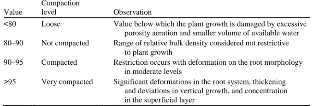
Table 9.1 Reference values for relative compaction from Oxisols under no-tillage conditions in southern Brazil

Compaction

Value level Observation

<80 Loose Value below which the plant growth is damaged by excessive

porosity aeration and smaller volume of available water

80–90 Not compacted Range of relative bulk density considered not restrictive

to plant growth

90–95 Compacted Restriction occurs with deformation on the root morphology

in moderate levels

>95 Very compacted Significant deformations in the root system, thickening

and deviations in vertical growth, and concentration in the superficial layer

Adapted from Marcolin (2009)

However, for the Oxisols samples studied by Marcolin and Klein (2011), no signi-ficant influence was found on the maximum bulk density, once the non-surface layer organic material contents, even in long-term no-tillage, were low (<3 %).

As mentioned earlier, cultivated soils have a bulk density ranging from 0.9 to 1.8 Mg m 3 due to their mineralogical and texture characteristics. Soils with the same mineralogical composition and texture may also present a wide range. For example, a clayey soil (ffi700 g kg 1 clay) may show a bulk density from 0.92 Mg m 3 in natural conditions to 1.3 Mg m 3 when intensively tilled (Klein 2012).

These differences in bulk density and the wide range cause difficulties for comparing results, even for other parameters obtained indirectly from the bulk density. The concept of relative bulk density consists of dividing the bulk density from the field by the maximum bulk density obtained by the Proctor test.

Relative compaction ¼

soil bulk density

100

maximum soil bulk density

Establishing optimal or critical values for plant development is a constant search. In this sense, through the compilation of research results and the relative compaction in which these studies were conducted, the table below was obtained to provide references values to quantify the physical quality of Oxisols (Table 9.1).

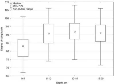
The assessment of Oxisols under no-tillage conditions (Fig. 9.4) demonstrates that the relative compaction in the 0–5 cm layer is below 90; that is, in loose conditions and in deeper layers, the average of most of the samples is above 90, indicating the state of compaction. The challenges ahead are to assess the behavior of plants in different compaction conditions, always considering the soil water content, which minimizes the effects of compaction and draws boundaries and models for soils different from Oxisols.

The opportunity to apply the relative compaction for the evaluation of the soil physical quality, notably in Brazil, is very large and easy to apply. Using equations as shown in Fig. 9.3, the use of relative compaction (RC) is a methodology easily performed, which is inexpensive and conceptually easily to understand; for this reason, it is considered a methodology that will be widely adopted.

Fig. 9.4 Relative compaction from Oxisol samples (94 per layer) under no-tillage conditions

9.4

S-Index

Among indicators of soil quality, the index proposed by Dexter and Bird (2001) and Dexter (2004) enables the physical qualities of soil (workability, permeability, structure stability, etc.) to be investigated, and should be particularly effective for providing information on the soil’s hydric functioning. This index is the slope (S) of the soil-water retention curve (SWRC) at its inflection point. It is determined for the SWRC when the gravimetric water content (W ), a function of soil-water suction (h) and expressed using the van Genuchten equation, is plotted with the natural logarithm of h. In this study, we use W to denote the gravimetric water content, rather than θ, as in Dexter and Bird (2001), to be more consistent with the literature, since θ usually represents the volumetric water content. As for the van Genuchten equation (van Genuchten 1980), which was written for θ, it remains valid for W.

Dexter (2004) derived the expression of the slope of the SWRC analytically to calculate the value of S, thus leading to the following expression:

S ¼

1 ð 1þmÞ

n ð Ws Wr Þ 1 þ

m

ð9:1Þ With m and n, the fitted dimensionless shape parameters of the van Genuchten equation; and Ws and Wr, the saturated and residual gravimetric water contents of the van Genuchten equation, respectively, measured in grams of water per g of oven-dried soil. This characteristic of the SWRC was considered by Dexter (2004) as a physical parameter (S-index) of the physical quality of soil. Dexter (2004) showed

that it was related to the texture, bulk density, organic matter content, and root growth of soil. Since its early developments, the S-index has been used by many

authors (Tormena et al. 2008). AU1 Dexter and Bird (2001), however, noted that there were two

possible inflection

points depending on whether W is plotted against log(h) or against h. They reported that the two inflection points are in close proximity for soils with a narrow pore-size distribution. This explains why they used the inflection point of curves of W vs. log (h), believing this was an estimate of air entry into granular materials which were considered in their study (Dexter and Bird 2001). Another point not raised by Dexter and Bird (2001) concerned their choice for computing the slope in a graph W vs. ln(h) of the W curve as a function of h according to the van Genuchten equation, instead of the slope of the W curve vs. ln(h), which would have been mathematically more consistent.

In this part of chapter, we discuss the choice of Dexter and Bird (2001) and compare the S-index with the slope of the SWRC at its inflection point when it is expressed as a function of the independent variables h, ln(h), or log(h). The equations developed are applied to a non-compacted and compacted soil and the resulting values of the slope are compared to the S-index.

9.4.1

Theory

Expression of W According to h, ln(h), and log(h)

On the basis of the van Genuchten equation (van Genuchten 1980), W can be expressed as:

h

i

m^ ¼ ^ þ ð α^ Þn^ þ ^ ð : Þ W Ws Wr 1 h Wr 9 2

with W the gravimetric soil water content (g g 1 ^ 1); Ws, the measured gravimetric

saturated soil water content (g g ); Wr, the fitted residual gravimetric soil water content (g g 1); α^ , the fitted scaling parameter (kPa 1); and n^ and m^ ¼ 1 1=n^, dimensionless fitted shape parameters. In order to facilitate presentation, Eq. 9.2

can be represented as:

^

n^, α^ , m^

ð9:3Þ W ¼ g h Ws, Wr,

with g being W as a function of h, given that parameters Ws (g g 1 ), W^ rð g g 1Þ, n^

(dimensionless), α^ hPa 1 , and m^ (dimensionless) are known. The circumflex on a letter is used to identify a fitted parameter value. m^ can also be fitted, but in this study, it was signed with Mualem (1976) constraint ð¼ 1 1=bnÞ.

Similarly, W vs. ln(h) can be represented by f using Eq. 9.2 as: ^ , n^1, α^1, m^1 W θ ¼ f ln ð h Þ θs, θ r1 ¼ f ln ð hÞ Ws, ^ ð9:4Þ W r1, n^1, α^1, m^1 for h 1, ^ ð g g 1 Þ, n^1 (dimensionless), α^ 1 hPa 1 , and m^ 1

with the fitted parameters W r1

(dimensionless), while W vs. log(h), can be represented by k, using Eq. 9.2, as:

W ¼ k logðh Þ

^

, m^1 for h 1, ð9:5Þ Ws, W r1, n^1, α^ 2

with α^ 2 the only new fitted parameter such as α^ 2 ¼ α^ 1 ln 10, the other fitted

parameters being identical to those determined for f.

Derivation of the SWRC to Obtain the Inflection Point

Taking Eqs. (9.3), (9.4), and (9.5) as general representations of the WRC and using Eq. 9.4, we can write the following derivatives:

g ¼

dh

¼ m^ n^ α^ n^ _{Ws W}^_r h_{1þ ðα^hÞn^} i _hn^

1 ð9:6Þ

dW m^ 1

with g the first derivative of W in relation to h,

f_

dW

ð ð h ÞÞ ¼

_d

ln

_W

^

r1

h

1 þ ð α^ 1lnð hÞÞ^n1 i

lnðh

Þ

^n 1 1 ð9:7Þ ¼ m^1^n1 α^ 1n^1 Ws _m^ 1 1

with f

_

the first derivative of W in relation to ln (h), and:

_ ¼

dW

k d log h

ð ð ÞÞ

h

1 þ ð α^ 2logð h ÞÞ^n1 i m^1 1 ¼ m^1n^1 α^ 2n^1 Ws W

^

r1 logð hÞ^n11 ð9:8Þ _

with k the first derivative of W in relation to log (h).

It is important to state that f

_

¼ dW=dð lnð h ÞÞ cannot be computed by simply applying the chain rule from Eq. 9.3, because the parameters determined by fitting either g (Eq. 9.3) or f (Eq. 9.4), subjected to Eq. 9.2, are not necessarily the same. This can be also said for functions g (Eq. 9.3) and k (Eq. 9.5), except

_ _

that, here, the only difference between f and k is the magnitude of the scaling parameters α^ 1 and α^ 2.

It is known that any continuous and differentiable mathematical function has its inflection points located where the second derivative is null throughout its real domain. Thus, at the inflection points for function g, we can set:

g€ ¼ dh2 ¼ m^ n^α^ n^ _W s W^r ð m^ n^ n^ Þ α^ n^ h1þ ðα^hÞn^ i h2n^ 2 þ ðn^ 1Þ d2W m^ 2 ¼

h

n^ 2

h

1

þ ðα^

hÞ

n^

i

m^ 1 _{¼ 0}

dT2 ¼ m^n^ α^n^ θs-θ^r ð m^ n^ n^Þ α^ n^ h1 þ ðα^ TÞn^ i T2 n^ 2 9:9 d2θ

m^ 2

þð n^ 1Þ Tn^2 h 1 þ ð α^ TÞ n^

i

m^ 1

ð Þ ¼ 0

with €g, the second derivative of W in relation to h. After simplifying Eq. (9.9), we obtain:

ð

m^

n^

n^ Þ α^ n^

h1þ ðα^hÞn^im^

2

h

2n^ 2

þ ð

n^

_{1Þ h}n^

2

h1þ ðα^hÞn^im^

1¼₀ ð9:10Þ Equation 9.10 can be solved for h to obtain the precise location of its inflection point (h)i as follows:

ð h Þi ¼ 1 1

ð9:11Þ α^ ðm^ Þn^

Similarly, we can compute the second derivative of Eqs. (9.7) and (9.8) to obtain:

ð lnð h ÞÞi ¼ 1 ð m^ 1Þ 1 ð9:12Þ n^ ₁ α^ 1

with (ln(h))i, the inflection point of W vs. ln(h), and:

ð logð h ÞÞi ¼ 1 ð m^ 1Þ 1 ð9:13Þ n^ 1 α^ 2

with (log(h))i, the inflection point of W vs. log(h).

Calculation of the Slope at the Inflection Point of the SWRC

The slope, Sh, from function g (Eq. 9.3) at its inflection point (Eq. 9.11) is obtained

. Sh ¼ ð α^ Þðn^ ^ Þ m^ ð 1 þ m^ Þ m^ 1 : ð9:14Þ 1Þ Ws W r ðm^

Similarly, the slope, Sln(h), from function f (Eq. 9.4) at its inflection point (Eq.

9.12), is obtained by substituting Eq. (9.12) into Eq. (9.7): ^ ð m^ 1Þ m^ 1 ð 1 þ m^ 1Þ m^ 1 1 : ð9:15Þ SlnðhÞ ¼ ðα^ 1Þð n^ 1 1Þ Ws W r1

The slope, Slog(h), from function k (Eq. 9.5) at its inflection point (Eq. 9.13) is

obtained by introducing Eq. (9.13) into Eq. (9.8): ^ ð m^ 1Þ m^ 1 ð 1 þ m^ 1Þ m^ 1 1 : ð9:16Þ

S

logðh Þ ¼ ðα

^

2Þð

n^

1

1

Þ

W

s

W

r1

9.4.2

Application to a Case Study

The equations developed in this study were applied to samples from a cultivated soil where compacted layers were identified (Santos et al. 2011). The soil studied was a clayey Ferralsol (Oxisol) according to the IUSS-WRB (2006) soil classification. It was located on a private farm (latitude 16.493246 S, longitude 49.310337 W, and altitude 776 m), near the “Embrapa Arroz e Feija˜o Agricultural Research Center”, at Santo Antoˆnio de Goia´s, GO, Brazil. The native vegetation was a typical Cerrado until 1985. After clearing the land, the soil was occupied by annual crops with conventional tillage for 2 years and then by a pasture of Brachiaria decumbens Stapf cv Basilisk. The soil was managed according to intensive animal grazing without any addition of fertilizer, which led to a compaction of the topsoil. In 2006, soil cores were collected with stainless steel 100 cm3 cylinders (diameter ¼ 5.1 cm, height ¼ 5.0 cm) in the compacted 0–5 cm and non-compacted 70–75 cm layers (Table 9.2). The higher bulk density found in the 0–5 cm layer is caused by soil compaction, since this type of soil, under native vegetation, exhibits a uniform bulk density profile according to depth, with a bulk density near to 1.0 g cm 3 (Santos et al. 2011).

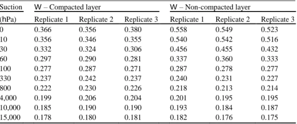
Gravimetric water contents (W in g g 1) at 10, 30, 60, 100, 330, 800, 4,000, 10,000, and 15,000 hPa were determined in triplicate for the two layers studied (Table 9.3), using the centrifuge method (Bruand and Prost 1987). A SWRC was fitted using the van Genuchten equation (van Genuchten 1980) (see Eq. 9.2) to the

different water contents measured for the compacted and non-compacted layers, using h, ln(h), or log(h) as the independent variable. The Solver routine embedded

^ α^^ ^

in Microsoft Excel was used to obtain the fitting parameters W r , , n , and m (Table

9.4). During the fitting process, Ws was taken as the mean value of the three

saturated water contents measured (Reatto et al. 2008): 0.367 g g 1 and 0.544 g g 1 for the compacted and non-compacted layer, respectively, and therefore was not adjusted.

At this point, it should be remembered that Dexter and Bird (2001) and Dexter (2004) derived the S-index formulation from the slope of SWRC plotted in a ln scale, and the result was transformed to a log scale by multiplying it by ln 10; this log scale was then used. In order to compare and discuss the location of the inflection point according to the independent variable used, we applied the equations developed here

Table 9.2 Principal physical and chemical properties of the 0–5 cm compacted and 70–75 cm non-compacted layers selected in the studied soil

Particle size distributiona

Soil Clay Silt Sand Organic carbona Bulk densityb

Compacted 485 71 444 0.70 1.27 Non-compacted 549 72 380 0.16 1.03 a g kg 1 b g cm 3

Table 9.3 Gravimetric soil water content (W g g 1) of the cores originating from the 0–5 cm

compacted (C) and 70–75 cm non-compacted (NC) layers according to the suction (hPa)

Suction W – Compacted layer W – Non-compacted layer

(hPa) Replicate 1 Replicate 2 Replicate 3 Replicate 1 Replicate 2 Replicate 3

0 0.366 0.356 0.380 0.558 0.549 0.523 10 0.356 0.346 0.355 0.540 0.542 0.516 30 0.332 0.324 0.306 0.456 0.455 0.432 60 0.297 0.290 0.281 0.337 0.360 0.333 100 0.277 0.287 0.271 0.287 0.278 0.277 330 0.237 0.242 0.237 0.240 0.231 0.227 800 0.222 0.230 0.226 0.218 0.213 0.214 4,000 0.199 0.206 0.204 0.201 0.195 0.195 10,000 0.185 0.190 0.190 0.193 0.184 0.187 15,000 0.178 0.180 0.181 0.182 0.176 0.175

and those of Dexter and Bird (2001) and Dexter (2004) to water retention properties found for compacted and non-compacted soils (Table 9.4).

The S-index computed using Eq. 9.1 and multiplied by ln 10, according to Dexter (2004), was 0.082 and 0.329 for the compacted and non-compacted soils, respectively. Using Eq. 9.16, the slope at the inflection point of the SWRC, expressed according to log(h) as the independent variable, was 0.081 and 0.326 for the compacted and non-compacted soils, respectively. These values are very close to the S-index computed as described by Dexter (2004). Thus, using an equation of W fitted with h as the independent variable and plotted with log(h) as abscissa, or an equation of W fitted with log(h) as the independent variable and plotted according to log(h), the slopes of the two curves at the inflection point are very similar. This could be expected, since the experimental points remain at the same place in the W - log(h) graph regardless of the independent variable used for the equation to describe the SWRC. Consequently, the slope at the inflection point of the SWRC computed according to Dexter (2004) who leads to the S-index and is used by many authors, would have been similar using Eq.

9.16 instead of Eq. 9.1.

On the other hand, the location of the inflection point of the curve of W vs. h, and the slope of the curve at this point, have more physical meaning than the corresponding values computed by Dexter (2004). The value of h at the inflection point can be considered as the “breakthrough” matrix potential at which air

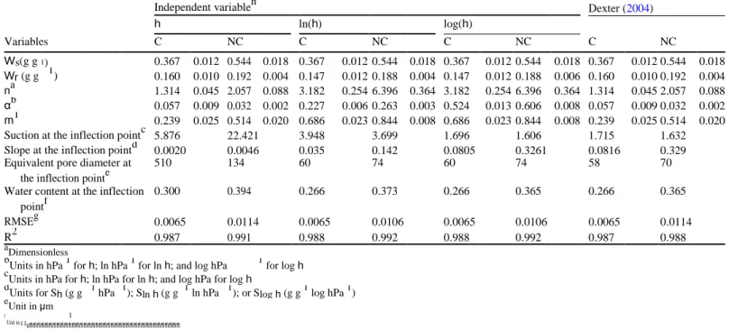
Table 9.4 Fitted parameter values for W vs. h, ln(h), or log(h), and corresponding inflection points and S-values for the 0–5 cm compacted (C) and 70–75 cm non-compacted (NC) layers

Independent variableh

Dexter (2004)

h ln(h) log(h) Variables C NC C NC C NC C NC Ws(g g1) 0.367 0.012 0.544 0.018 0.367 0.0120.544 0.018 0.367 0.0120.544 0.018 0.367 0.0120.544 0.018 Wr (g g 1) 0.160 0.010 0.192 0.004 0.147 0.0120.188 0.004 0.147 0.0120.188 0.006 0.160 0.0100.192 0.004 na 1.314 0.045 2.057 0.088 3.182 0.2546.396 0.364 3.182 0.2546.396 0.364 1.314 0.0452.057 0.088 αb 0.057 0.009 0.032 0.002 0.227 0.0060.263 0.003 0.524 0.0130.606 0.008 0.057 0.0090.032 0.002 m1 0.239 0.025 0.514 0.020 0.686 0.0230.844 0.008 0.686 0.0230.844 0.008 0.239 0.0250.514 0.020

Suction at the inflection pointc 5.876 22.421 3.948 3.699 1.696 1.606 1.715 1.632

Slope at the inflection pointd 0.0020 0.0046 0.035 0.142 0.0805 0.3261 0.0816 0.329

Equivalent pore diameter at 510 134 60 74 60 74 58 70

the inflection pointe

Water content at the inflection 0.300 0.394 0.266 0.373 0.266 0.365 0.266 0.365

pointf RMSEg 0.0065 0.0114 0.0065 0.0106 0.0065 0.0106 0.0065 0.0114 R2 0.987 0.991 0.988 0.992 0.988 0.992 0.987 0.988 a Dimensionless b

Units in hPa 1 for h; ln hPa 1 for ln h; and log hPa 1 for log h

c

Units in hPa for h; ln hPa for ln h; and log hPa for log h

d

Units for Sh (g g 1 hPa 1); Slnh (g g 1 ln hPa 1); or Slogh (g g 1 log hPa 1)

e Unit in μm f 1 Unit in g g_{sffiffiffiffiffiffiffiffiffiffiffiffiffiffiffiffiffiffiffiffiffiffiffiffiffiffiffiffiffiffiffiffiffiffiffiffiffiffiffi} n ^ g RMSE¼ 1=N X Wi 2 1 Wi in g g i¼1 h

The standard errors for Ws were calculated directly from the measured values. Those for Wr, n, α, and m originated from the analysis of variance of errors due to regression when fitting these parameters

penetrates throughout the soil. The slopes at the inflection point of the SWRC, using Eq. 9.14 with h as the independent variable, were 0.0020 and 0.0046 for the compacted and non-compacted soil, respectively. These values are 41 and 72 times smaller than the corresponding S-index values (Table 9.4), respectively. Suction at the corresponding inflection point using Eq. 9.11 was 6 and 22 hPa for the compacted and non-compacted soil, respectively; though, according to Dexter (2004) these values were 52 and 43 hPa (Table 9.3).

Using Jurin’s law (Bruand and Prost 1987) we computed the equivalent pore diameter corresponding to the suction at the inflection point of the SWRC (Table

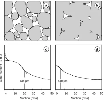
9.4). The results showed a close equivalent pore diameter for compacted and non-compacted soil at the inflection point when the SWRC was plotted with ln(h) or log(h) as the independent variable (60 and 74 μm, respectively) and according to Dexter (2004) (58 and 70 μm, respectively). On the other hand, the equivalent pore diameter at the inflection point of the SWRC was about four times higher for compacted soil (510 μm) than for the non-compacted soil (134 μm) when the SWRC was plotted with h as the independent variable (Table 9.4).

In contrast to what is indicated by the S-index, however, air would penetrate throughout the soil at a smaller suction, and, consequently, for a larger equivalent pore diameter for compacted than for non-compacted soil. This result may appear surprising since compaction leads to smaller porosity with a shift of the inflection point on the SWRC to a larger suction. The effects of compaction on pore geometry are difficult to understand, since they depend on the structure and related pore types prior to compaction, on soil composition and water content, and on the intensity of compaction.

Beneath native vegetation, the soil studied had a weak macrostructure and a pronounced granular structure at the micrometer scale (Balbino et al. 2002). Since the structure of non-compacted soil is considered to be similar to the structure under native vegetation, its theoretical SWRC would be a bimodal curve with two inflection points: (i) one corresponding to pore draining resulting from micro-aggregate assemblage and occurring for a very low suction of several hPa, such as for coarse sandy soils, and (ii) one corresponding to pore draining resulting from the assemblage of elementary particles in micro-aggregates and occurring for values of several hundred hPa. Because of the difficulty to correctly measure water retention of the soils studied at several hPa, only the second inflection point is usually measured (Balbino et al. 2002).

When soil is compacted, the pores resulting from the assemblage of micro-aggregates are transformed into smaller pores. The resulting SWRC contains one inflection point which is related to a continuous distribution of equivalent pore diameters from the smaller pores, which were distorted by compaction, to those resulting from the assemblage of the elementary particles in microaggregates. Figure 9.5, which is based on the results of several studies on similar soils, illustrates how using such a transformation of porosity makes it possible to pass from a SWRC, with a given inflection point and its related equivalent pore diameter for a non-compacted soil, to another SWRC, with an inflection corresponding to a larger equivalent pore diameter for compacted soil.

W a te r c o n te n t ( g g -1 ) a b c d 134 µm 510 µm 0 10 20 30 40 50 0 10 20 30 40 50

Suction (hPa) Suction (hPa)

Fig. 9.5 Schematic representation of the structure of the non-compacted (a) and compacted soil (b), and the soil water retention curve corresponding to the non-compacted soil (c). The portion of the curve that relates to the pores resulting from the assemblage of the micro-aggregates (white in (a) and dashed curve in (c)) was not measured. The soil water retention curve of the compacted soil (d) is shown with the value of the equivalent pore diameter in μm at the inflection point

Finally, our results question the value of S as a possible index to determine the physical quality of soil. The values of h at the inflection point determined for compacted and non-compacted soil are low, thus corresponding to water content close to saturation, which should not be optimal for soil tillage.

The expression of the SWRC according to ln(h) or log(h) as the independent variable, instead of h, leads to different values of the index. Computing the S-index when the SWRC is expressed with h as the independent variable is both mathematically and physically consistent. We also show that, independent of the consistency of the approach, the discussion of the physical properties of the soil can be limited according to the independent variable used. For the soil selected, our results, in fact, show that calculation of the S-index when it is expressed with h as the independent variable significantly increases the relevance of the analysis com-pared to the range of the S-indices when it is expressed as proposed by Dexter and Bird (2001). Further work will aim to determine in which proportion the S-index is affected for a large range of soils and to verify if the use of h as the independent variable effectively increases sensitivity of the analysis.

9.5 Least Limiting Water Range (LLWR)

The term “Least Limiting Water Range” (LLWR) was used (Letey 1985; da Silva et al. 1994) to define the region bounded by the upper and lower soil water content over which water, oxygen, and mechanical resistance become major limitations for root growth. It is delimited by the supply of oxygen to the roots at the wet end, and by the supply of water to the roots and mechanical resistance to root growth at the dry end.

The computation of the LLWR for plant growth requires that functional relation-ships be obtained between water content (θ) and each of the following properties: water potential, mechanical resistance, and aeration. To compute the LLWR, the matric potential at field capacity and a limiting value of aeration must be defined at the wet end of the range, and a limiting value of mechanical resistance and the matric potential at the permanent wilting point must be defined for the dry end. The water contents are then determined at the limiting values. The smallest range between these limiting water contents is defined as the LLWR. The critical limits defining the LLWR were (1) soil water contents at field capacity (ψ ¼ 0.01 MPa) and permanent wilting point (ψ ¼ 1.5 MPa); (2) air filled porosity less than 10 %; and (3) soil strength >2.0 MPa.

Undisturbed soil samples are used to determine the functional relationships. The sampling has to encompass the variation of structural conditions, expressed by the soil bulk density, of the soil(s) under study, in order to model properly the water release curve (WRC, θ versus ψ), and the soil resistance curve (SRC, soil strength as a function of soil water content and bulk density). Once the functional relation-ships have been defined, the LLWR computation is performed, as demonstrated in Fig. 9.6. The critical limits of water contents at field capacity and permanent wilting point are obtained from the WRC (Fig. 9.6a, b) for each soil sample. Similarly, in dry soils, the mechanical resistance may reach limiting values at low values of ψ before the permanent wilting point is reached. In the dry end, depending on the structural condition of the soil, the θWP can be substituted by the water content at which the soil strength (θSR) reaches the

critical value previously defined (Fig. 9.6d). In soils with degraded structure, the wet end of the LLWR is commonly determined by the θAFP instead of θFC (Fig. 9.6e). In

these cases, at θFC, the plant growth is theoretically conditioned by the restricted

diffusion of oxygen in the soil. The air-filled porosity is strongly dependent on the soil structural condition, being linear and negatively related with the soil bulk density (ρb).

Figure 9.3 demonst-rates that θAFP substitutes θFC, while θSR substitutes θWP, starting

from values ρb ¼ 1.40 g cm 3. In this condition, the LLWR is strongly reduced until it

reaches a value of zero. The LLWR is zero when the water content values at the wet end and at the dry end are numerically the same. The critical bulk density of the soil (ρbc) is

defined as the value of ρbc at which LLWR ¼ 0. For the soil illustrated in Fig. 9.6e, the

LLWR ¼ 0 when the ρbc ¼ 1.55 g cm 3.

LLWR integrates four static soil characteristics (aeration, field capacity, soil mechanical resistance, and permanent wilting point) into a single variable.

Fig. 9.6 Determination of the critical values of the variables FC, WP, AP, and SR that define the LLWR

Dynamic soil characteristics, such as parameters describing the transport of water or oxygen, are not taken into account. Limiting soil resistance of the soil matrix, and therefore the calculated value of the LLWR, is of limited relevance to compacted soils with an abundance of macropores, because root growth occurs mainly in these macropores, rather than in the soil matrix. Limiting values are time-consuming to measure, and the impact of some characteristics – particularly those of soil

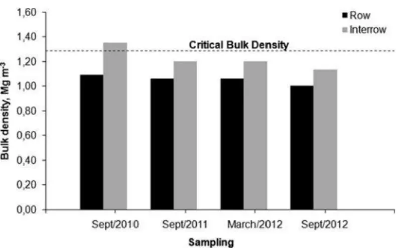
Fig. 9.7 Soil bulk density (ρb) in different sampling seasons in an Oxisol under no-tillage. The

dotted line indicates the critical bulk density equal to 1.29 Mg m 3

resistance and aeration - on the extent of rate reduction of those physiological processes that have the greatest influence on yield is not well-defined. The variation in this reduction among different crops is largely unexplored. Although interaction between limiting characteristics (e.g., the effect of reduced aeration on limiting values of soil resistance) could be accounted for in the concept of the LLWR, this interaction is generally not considered.

An example of an application of the LLWR for the control and monitoring of the soil physical quality is shown in Fig. 9.7. This study was conducted on a commercial grain production farm in northwestern Parana State, in the municipality of Maringa (23 3004000 S, 51 5904800 W), in a soil classified as Oxisol (Rhodic Ferralsol), in the clay textural class (800 g kg 1 clay content). The land is under a no-tillage system since 1979 with a crop rotation including soybeans, corn, wheat, and oats. Corn and soybeans were sown using furrow opener drills, while oats and wheat were sown with double-disc coulters. The LLWR was evaluated as described by da Silva et al. (1994) and Betioli Junior et al. (2012). The critical bulk density value (ρbc, the soil

bulk density [ρb] value in which LLWR ¼ 0) was 1.29 Mg m 3. Sampling for

monitoring surface soil physical quality was performed immediately after the harvest of corn in September 2010, September 2011, and September 2012, and after the soybean harvest in March 2012, at 40 locations along a transect crossing 40 crop rows. At each location (40 in rows and 40 in the adjacent inter-row positions), at 0– 10 cm depth, undisturbed soil cores (50 mm high 70 mm in diameter) were collected. We sampled this layer because it is the most biologically active zone, and where soil disturbance associated to furrow opening during seeding occurs under no-tillage.

The critical bulk density estimated from LLWR can be used as a reference for the monitoring of soil physical quality and only requires the measurement of soil ρb. The determination of ρb is simple, requires minimal instrumentation, is

relatively inexpensive, and can be performed at the farm level. Increasing values of ρb over ρbc values are indicative of greater physical limitations of the soil, since

excessive soil resistance to root penetration or reduced aeration may limit plant growth due to the natural variability of soil water content. As shown in Fig. 9.7, in no-till there is a consistent and systematic difference between inter-row and row conditions, with soil physical quality being more favorable in the row area. The favorable soil physical conditions within the rows may be attributed to the loosening action of the chisel coulters of the no-till seeder, which open the soil to a depth of 0.12 m. The average values of ρb indicated that only in September 2010 did ρb

exceed ρbc in the inter-row positions, yet this value was not high enough to require

remedial action. In all subsequent sampling, ρbc systematically exceeded ρb,

suggesting that a reduction in ρb within rows may due to soil’s physical resilience associated with wetting and drying cycles, effects of root crops, and the residual effect of the disturbance of the soil by chisel coulters.

To revisit Einstein´s quote, these are the answers for this year’s “exam”. For sure, soil physics will continue to attract new people, and much improved answers will be available for the same questions in the near future.

References

Balbino LC, Bruand A, Brossard M et al (2002) Changes in porosity and microaggregation in clayey Ferralsols of the Brazilian Cerrado on clearing for pasture. Eur J Soil Sci 53:219–230 Ball BC, Batey T, Munkholm L (2007) Field assessment of soil structural quality – A development of the Peerlkamp test. Soil Use Manage 23:329–337

Bruand A, Prost R (1987) Effect of water content on the fabric of a soil material: an experimental approach. J Soil Sci 38:461–472

Betioli Ju´nior E, Moreira WH, Tormena CA, Ferreira CJB, da Silva AP, Giarola NFB (2012) Intervalo hı´drico o´timo e grau de compactac¸a˜o de um Latossolo Vermelho apo´s 30 anos

sob plantio direto. Revista Brasileira de Cieˆncia do Solo 36:971–982. doi:

10.1590/S0100-06832012000300027

da Silva AP, Kay BD, Perfect E (1994) Characterization of the least limiting water range of soils. Soil Sci Soc Am J 58:1775–1781

Dexter AR (2004) Soil physical quality: part I, theory, effects of soil texture, density, and organic matter, and effects on root growth. Geoderma 120:201–214

Dexter AR, Bird NRA (2001) Methods for predicting the optimum and the range of soil water contents for tillage based on the water retention curve. Soil Tillage Res 57:203–212

Giarola NFB, Silva AP, Tormena CA, Guimara˜es RML, Ball BC (2013) On the visual evaluation of soil structure: the Brazilian experience in oxisols under no-tillage. Soil Tillage Res 127:60– 64

Guimara˜es RML, Ball BC, Tormena CA (2011) Improvements in the visual evaluation of soil structure. Soil Use Manage 27:395–403

International Union of Soil Science Working Group (2006) World reference base for soil resources 2006: a framework for international classification, correlation and communication. FAO, Rome

Klein VA (2012) Fı´sica do Solo. EDIUPF, 2ª Ed. 240 p, Pelotas, Brazil

Letey J (1985) Relationship between soil physical properties and crop production. Adv Soil Sci 1:277–294

Marcolin CD (2009) Indicadores da qualidade fı´sica de solos sob plantio direto obtidos por func¸o˜es de pedotransfereˆncia. Tese (Doutorado em Agronomia) – FAMV-UPF, 183 p Marcolin CD, Klein VA (2011) Determinac¸a˜o da densidade relativa do solo por uma func¸a˜o

de pedotransfereˆncia da densidade do solo ma´xima. Acta Sci Argon 33:349–354

Mualem Y (1976) A new model predicting the hydraulic conductivity of unsaturated porous media. Water Resour Res 12:513–522

Peerlkamp PK (1959) A visual method of soil structure evaluation. Medelingen von de Landbouwhogeschool en Opzoekingstations van de Staat te Gent Deel XXIV 24:216–221 Reatto A, Silva EM, Bruand A et al (2008) Validity of the centrifuge method for determining the

water retention properties of tropical soils. Soil Sci Soc Am J 72:1547–1553

Santos GG, Marcha˜o RL, Silva EM et al (2011) Qualidade fı´sica do solo sob sistemas de integrac¸a˜o lavoura-pecua´ria. Pesq Agropec Bras 46:1339–1348

Shepherd TG (2009) Visual soil assessment, vol 1. Field guide for cropping and pastoral grazing on flat to rolling country, 2nd edn. Horizons Regional Council, Palmerston North

van Genuchten MT (1980) A closed-form equation for predicting the hydraulic conductivity of unsaturated soils. Soil Sci Soc Am J 44:892–898