HAL Id: hal-01509782
https://hal-brgm.archives-ouvertes.fr/hal-01509782
Submitted on 18 Apr 2017
HAL is a multi-disciplinary open access
archive for the deposit and dissemination of
sci-entific research documents, whether they are
pub-lished or not. The documents may come from
teaching and research institutions in France or
abroad, or from public or private research centers.
L’archive ouverte pluridisciplinaire HAL, est
destinée au dépôt et à la diffusion de documents
scientifiques de niveau recherche, publiés ou non,
émanant des établissements d’enseignement et de
recherche français ou étrangers, des laboratoires
publics ou privés.
cross-shore and alongshore processes.
Arthur Robinet, Bruno Castelle, Déborah Idier, Vincent Marieu, Kristen
Splinter, Mitchell Harley
To cite this version:
Arthur Robinet, Bruno Castelle, Déborah Idier, Vincent Marieu, Kristen Splinter, et al.. On a
reduced-complexity shoreline model combining cross-shore and alongshore processes.. Coastal Dynamics 2017,
Jun 2017, Helsingør, Denmark. �hal-01509782�
ON A REDUCED-COMPLEXITY SHORELINE MODEL COMBINING CROSS-SHORE AND ALONGSHORE PROCESSES
Arthur Robinet1, Bruno Castelle2, Déborah Idier1, Vincent Marieu2, Kristen D. Splinter3 and Mitchell D. Harley3
Abstract
We present a new empirical shoreline evolution model integrating longshore and cross-shore processes. It is designed for wave-dominated sandy coasts and includes feedback between shoreline and wave dynamics. It can also take into account non-erodible (e.g. rocks, artificial structures) contours and complex wave propagation patterns through the coupling with the spectral wave model SWAN. While the longshore-transport-based modeling approach can reproduce the shoreline variability on large temporal scales, say from years to decades, inclusion of the equilibrium-based cross-shore model enables cross-shoreline variability to be addressed at the scales of changes in incident wave energy, say from hours to years. In this paper, the basic assumptions of the model are presented. The model is tested to synthetic cases before being applied to a real case scenario (Narrabeen Beach, Australia). Finally, guidelines for future model developments are given.
Key words: shoreline model, longshore transport, cross-shore transport, long-term modeling, SWAN model, sandy and
non-erodible rocky coasts
1. Introduction
In the context of global climate change and population growth, the littoral region is a particular hot-spot that is becoming increasingly topical and politically sensitive worldwide in a context of widespread erosion. Over the last few decades, a number of complex process-based models have been developed to simulate and further predict wave-dominated beach changes at event time scale. These models (e.g. Roelvink et al., 2009) can simulate storm-driven beach changes on short temporal and spatial scales. However, they cannot be used to predict shoreline evolution on long time scales (i.e. years, decades). Indeed these models still contain misspecified physics, these misspecifications cascading up through the scales resulting in an inescapable build-up of errors in long simulations. In addition these models are too computationally consuming to enable long-term simulations. Instead, reduced-complexity models can lead to more reliable long-term evolution than do parameterizations of much smaller-scale processes in process-based models, as evidenced in many geomorphological systems. For instance, on the one hand behaviour-oriented equilibrium-based models have been shown to hindcast shoreline change on cross-shore transport dominated beaches from hours to years with fair accuracy (e.g. Splinter et al., 2014). On the other hand, as far as longshore sediment processes are concerned, one-contour-line numerical models (e.g. Hanson, 1989, Ashton and Murray, 2006) can simulate longshore-drift-gradient driven changes that typically occur on longer timescales. The dynamics of most wave-dominated beaches is driven by both longshore and cross-shore processes acting at different levels according to local wave climate and geological features. Until now, cross-shore and longshore processes have been mostly addressed in isolation (Ashton and Murray, 2006; Yates et al., 2009; Davidson et al., 2013; Splinter et al., 2014). A fundamental step to increase our understanding of shoreline change from the time scales of hours (i.e. storm) to decades is to combine cross-shore and longcross-shore processes into a single reduced-complexity cross-shoreline model. In this paper, we develop such a model to simulate short- to long-term wave-driven shoreline change with reasonable computational
1BRGM, 3 avenue Claude Guillemin, 45100 Orléans, France. [email protected]; [email protected]
2CNRS, UMR 5805 EPOC, Pessac, France. [email protected]; [email protected] 3Water Research Laboratory, University of New south Wales, Sydney, Australia, [email protected];
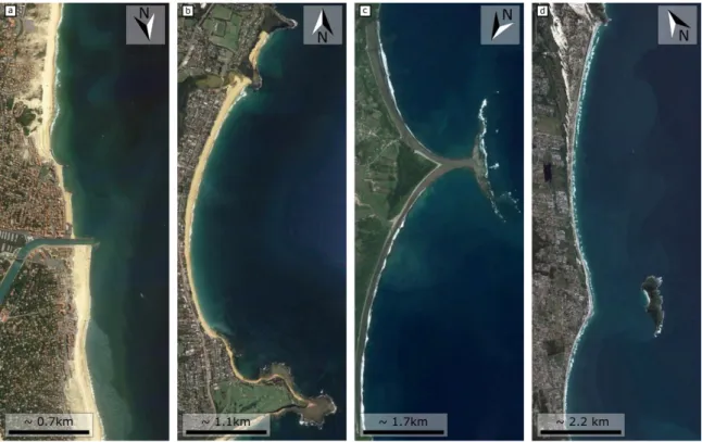
time (one day of computation time corresponds to 103-104 days of real time), with the overarching goal to quantify the respective contributions of cross-shore and longshore processes to the overall shoreline evolution along open and embayed beaches. Some additional features are implemented to design a model that can be applied to a wide range of wave-dominated coastal environments (Fig. 1). First, the model is coupled to the spectral wave model SWAN, thereby providing more accurate estimates of surf zone sand transport along complex coastline geometries where wave refraction and shadowing patterns prevail. Second, the definition of non-erodible areas is implemented to take into account the impact of headlands, offshore islands and breakwaters which are critical to model shoreline change along rugged and/or trained coasts (Fig. 1).
Figure 1. Examples of sandy coastlines with different, complex, geometries enforced by the geological settings (e.g. headlands, offshore islands) or coastal hard structures. a Hossegor-Capbreton beaches, France. b Narrabeen beach,
Australia. c Punta Uvita, Costa Rica. d Campeche beach, Brazil. Source: Google Earth
The development of the model (called LX-Shore) is described in section 2 and its main features are addressed in section 3 through two synthetic cases. Finally, in section 4 the model is tested against the real case of monthly shoreline change along Narrabeen Beach (south-eastern Australia) over a 9-yr period from 2005 to 2014. Conclusions are subsequently drawn in section 5.
2. Model Development 2.1. General overview
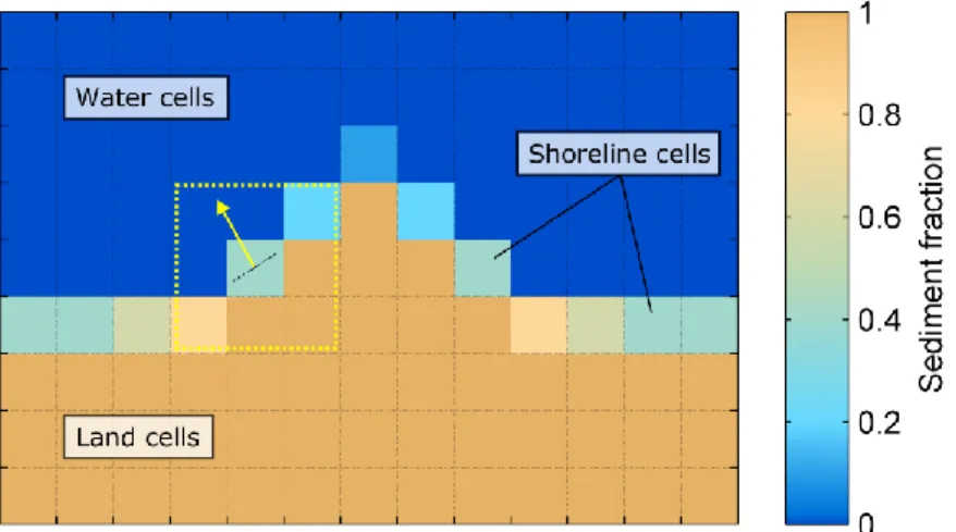
The shoreline model consists of a 2D plan-view model inspired by the pioneer work of Ashton et al. (2001) and Ashton and Murray (2006) (development of the Coastal Evolution Model, hereafter referred to as CEM), with some substantial differences such as the computation of breaking wave angle numerical schemes. The model addresses changes in sediment fraction F (ranging from 0 to 1) inside squared grid cells having a constant spatial resolution, dxy, of the order of 10 to 100 m (Fig. 2). Water cells are cells with F = 0, shoreline cells are cells with 1 ≥ F > 0 having an edge contact with at least one water cell, and land cells are the other cells. For each shoreline cell a shore-normal vector (represented by the yellow
arrow in Fig. 2) is estimated according to the horizontal and vertical gradients in sediment fraction calculated over a 3-by-3-cell sub-grid centered on the current cell (shown by the yellow dotted square contour in Fig. 2). Additionally, for each shoreline cell, an estimate of the shoreline position is computed using the shore-normal vector and sediment fraction. A specific interpolation method has been implemented to retrieve the entire shoreline by combining shore-normal vectors and the estimates of shoreline position. Changes in sediment fraction inside shoreline cells are estimated for each simulation time step according to the balance between incoming and outgoing sediment fraction induced by longshore and cross-shore sediment transport. One of the main assumptions underlying such an approach is that the shoreline changes result only from seaward and shoreward translation of a constant beach profile up to a finite depth named the shoreface depth Dsf as in Asthon and Murray (2006). Based on this assumption, it is
possible to make conversion between the model grid cell sediment fractions and sediment volumes. The maximum sediment volume a cell can contain is Vs,max = dxy2Dsf and the actual sediment volume contained
by a cell is Vs = FVs,max.
Figure 2. Example of a sediment fraction grid (F) with square grid cells of resolution dxy. The yellow dotted square contour indicates the 3-by-3-cell sub-grid used to compute the shore-normal vector represented by the yellow arrow
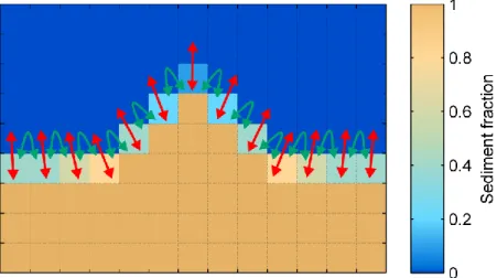
2.2. Longshore transport
Longshore sediment transport is calculated at each boundary between two shoreline cells (green double arrows in Fig. 3) using the formula of Kamphuis et al. (1991):
2 1.5 0.75 0.25 0.6 , 50
2.27
sin (2 )
(
)(1
)
s b p b b l sH T m
d
Q
p
(1) where Hs,b is the significant wave height at breaking, Tp the peak period, mb the beach slope, d50 the meansediment grain size, θb the breaking wave incidence angle, ρs and ρ respectively the sediment and water
density, and p the sediment porosity. This formula has been used in many coastal applications. In our study, it is used because the formula only requires the site characteristics (ρs, d50) with no further calibration.
2.3. Cross-shore model
The cross-shore sediment transport is calculated inside each shoreline cell (red double arrows in Fig. 3) using an adaptation of the ShoreFor model (Davidson et al., 2013) formulation proposed by Splinter et al. (2014). The ShoreFor model assumes that cross-shore shoreline displacements result from disequilibrium between the instantaneous dimensionless fall velocity at breaking (Ωb) and the equilibrium dimensionless
eq b
(2)The dimensionless fall velocity reads:
, s b b p
H
wT
(3)where w is the settling velocity. The equilibrium dimensionless fall velocity is computed using a weighted integration of the dimensionless fall velocity over a site-specific period (Φ) to the past which can vary from some days to hundreds of days depending on the characteristics of the beach (Davidson et al., 2013; Splinter et al., 2014). The shoreline change rate (dS/dt) is finally expressed as:
/ 0.5
dS dt
c
P
b
(4)where P is the wave energy flux at breaking, σΔΩ the standard deviation of ΔΩ (used to normalize ΔΩ), b a term added to encapsulate long-term processes not included in the ShoreFor model (e.g. constant sediment inputs and losses). The coefficient c+/- is either equal to c or cr if ΔΩ > 0 or ΔΩ < 0, respectively, where c is the rate parameter and r the erosion ratio. The coefficient Φ, c and b are the model free parameters and are obtained by an optimization procedure against shoreline measurements. The erosion ratio is calculated according to the balance between accretion and erosion forcing in a way that ensures that the ShoreFor model does not result in a shoreline change trend while the forcing has no trend (Splinter et al., 2014). With this formulation, the direction of the shoreline displacement (landward or seaward) is given according to the sign of the disequilibrium. The magnitude of the displacement is proportional to the product of the normalized disequilibrium with the incident wave energy flux. For a complete and detailed model description, the readers are referred to the work of Davidson et al. (2013) and Splinter et al. (2014).
Figure 3. Longshore transport (green double arrows) is estimated at each boundary between two shoreline cells while cross-shore transport (red double arrows) is estimated inside each shoreline cell
To keep a reasonable computing time applying the ShoreFor model to all shoreline cells, of which number and location evolve during the simulation, an adjustment of equation (3) has been done. Computing the dimensionless fall velocity disequilibrium at breaking would require to record one time series of past breaking wave conditions for each shoreline cell which in turn would be memory and time consuming. It would also be a complex process when new shoreline cells are created during the course of the simulation. Instead, in a first approach, we decided to compute a unique time series of dimensionless fall velocity
disequilibrium using the offshore wave data. P is still calculated using the breaking wave conditions at each shoreline cell. Thus, the direction of the shoreline displacement is given according to the offshore data while the magnitude remains dependent on breaking conditions.
2.4. Shoreline evolution
The net longshore sediment transport and cross-shore shoreline change rate predicted by the cross-shore model are converted into sediment fraction using the assumption that small positive or negative sediment balance inside a shoreline cell results in slight cross-shore translation of a constant beach profile. The sediment fraction variation resulting from longshore processes (dF1) is given by:
,in ,out ,max
(
l l)
l sQ
Q
dF
t
V
(5)where Ql,in and Ql,out are respectively the incoming and outgoing sediment transport and Δt the simulation
time step. The sediment fraction variation resulting from cross-shore processes (dFc) is given by:
c
dS dt
dF
t
dxy
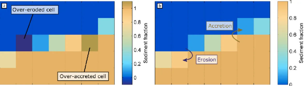
(6)The sediment fraction is updated by adding dFl and dFc at each time step and at each shoreline cell. In case of over-accreted shoreline cell (F > 1) the sediment fraction excess is spread into the water cell overlapping the most perpendicular direction to the shoreline (Fig. 4). Conversely, in case of over-eroded shoreline cell (F < 0) the sediment deficit is filled by taking sediment fraction from the land cell overlapping the most perpendicular direction to the shoreline (Fig. 4).
Figure 4. Illustration of empirical accretion and erosion laws applied to over-accreted (F > 1) and over-eroded (F < 0) shoreline cells, respectively
2.5. Wave module
Most of the large-scale empirical shoreline models use basic but fast methods to estimate the wave parameters at breaking. As long as the curvature of the coast is weak and the bathymetric contours remain parallel to the mean shoreline orientation these methods are satisfied. Such approaches however become unreliable when applied to complex coastline geometries, i.e. along rugged and/or trained coasts. In addition, a number of recent hybrid semi-empirical shoreline models (Idier et al., 2011, Van Den Berg et al., 2012, Kaergaard et al., 2013, Limber et al., 2017) have shown that using a refined wave modeling approach is crucial to improve the geometry and emergence time of shoreline instabilities. Here, the shoreline model has been fully coupled with the spectral wave model SWAN to obtain accurate wave conditions at breaking for all shoreline configurations. We also implemented simpler wave approaches. The
simplest one consists of applying the offshore wave conditions everywhere in the water domain with the exception of the shadowed areas, for which significant wave heights are set to 0 m.
2.6. Additional features
Similarly to the shoreline model of Kaergaard et al. (2013) a bathymetry reconstruction module has been implemented that updates the bathymetry at each time step according to the new shoreline. This bathymetry is used to compute the wave field with SWAN during the subsequent time step. The bathymetry consists of a grid having the same extent as the sediment fraction grid, but with a finer spatial resolution ensuring that the surf zone is not restricted to only one computational cell. A spatial resolution of 10 to 20 m is recommended to allow the SWAN model to accurately resolve wave breaking processes. A depth is estimated at each cell of the bathymetric grid overlapping the water domain. The depths are retrieved by projecting the shoreline over the bathymetric grid and propagating offshore a constant beach profile (e.g. a Dean profile). Finally, non-erodible areas can be defined in the model to take into account the impact of headlands, offshore islands and breakwaters which could block longshore sediment transport or modify the wave field through attenuation and refraction.
3. Model Capabilities: Synthetic Cases
First, two idealized application cases are described. These applications focus on the coupling with SWAN and the implementation of non-erodible coasts. Thus, we switch off the cross-shore processes, which typically needs real wave time series to compute the free parameters.
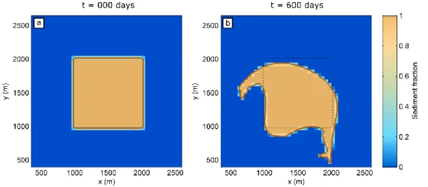
3.1. Square island
The first synthetic case consists of a square sandy island (Fig. 5a) exposed to a stationary wave forcing. The significant wave height is set to 1.5 m, the peak period to 10 s and the wave direction to NNE (22.5° TN). The simulation is performed using the coupling with the SWAN model over a 600-day period with a 6-h time step and a 50-m grid resolution for the sediment fraction.
Figure 5. Shoreline change after 600 days of simulation using the developed shoreline model combined with the SWAN model. Brown line shoreline position. Dotted black line initial shoreline position
The final island shape (Fig. 5b) shows that using the coupling with SWAN the model simulates a realistic bending of the island forming 2 spits migrating downdrift, together with the smoothing of the NE edge of the island. Not surprisingly, the sand spit is longer along the eastern side than along the northern side as the angle of wave incidence and the resulting longshore drift are larger. In addition, the model shows some
substantial changes in the SW part of the islands as SWAN allows waves to refract and break along the sheltered sides of the island.
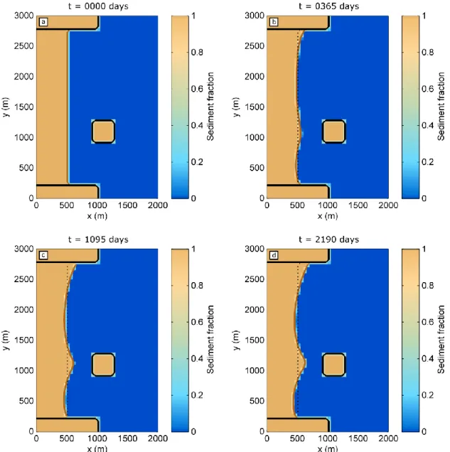
3.2. Rectilinear embayed beach with asymmetrical waves and offshore island
The second synthetic case consists of a rectilinear beach bordered by two rectangular non-erodible headlands at the N and S ends with the implementation of a non-erodible square island offshore (Fig. 6a). An asymmetrical wave climate is applied at the offshore boundary of the water domain. Wave height and wave period are set constant and are equal to 1.5 m and 10 s, respectively. The wave direction randomly alternates between SE (135° TN) and ENE (67.5° TN). Note that the occurrence frequency of the SE wave direction is set to the double of the ENE wave direction to force a dominant wave direction. The simulation is conducted using the coupling with the SWAN model, a 6-h time step and a 50-m sediment fraction grid spatial resolution.
Figure 6. Shoreline change after 2190 days (~6 years) of simulation using the developed shoreline model coupled with SWAN. Brown line shoreline position. Dotted black line initial shoreline position. Black lines non-erodible areas
After a 1-yr simulation period a slight clockwise rotation of the beach is already noticeable with accretion at N and erosion at S (Fig. 6b). In addition, a salient develops along the shoreline located in the lee of the island. These evolution patterns persist over the entire simulation but decrease in magnitude after 3 years for the shoreline salient (Fig. 6c) and after 5 years for the rotation. After a 6-yr simulation period the shoreline reaches a dynamic equilibrium state (Fig. 6d).
The simulated beach rotation results from the combination of: disequilibrium between the initially E-facing straight shoreline and the idealized wave climates dominated by SSE waves causing a net N-oriented longshore sediment transport; and the presence of the headlands. The presence of the offshore island impacts the wave field with smaller breaking waves in the lee of the island and, in turn, a reduced longshore sediment transport. This alongshore gradient drives a systematic accretion and the formation of a salient facing the island.
This synthetic case highlights the ability of the model to account for detached and shore-attached non-erodible structures as well as the advantages of using SWAN to accurately simulate the wave field
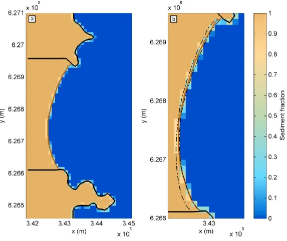
4. Coupling with the Cross-Shore Model: Application to Narrabeen Beach
To test the model coupling with the cross-shore transport, the model was applied to a real beach. The Narrabeen-Collaroy embayment (hereafter referred to as Narrabeen), NSW, Australia, is an ideal site to test the model because: a) it is one of the most extensively and continuously surveyed beaches worldwide with more than 40 years of data; b) shoreline changes at Narrabeen are driven by both longshore and cross-shore sediment transports although their respective contribution is still the subject of debate (Harley et al., 2015); c) most of the data are in open access (Turner et al., 2016); d) ShoreFor model has already applied to this site (Splinter et al., 2014).
Narrabeen beach is a 3.6-km long E-facing embayment with an almost uniform sediment granulometry (Turner et al., 2016). The sediment consists of fine to medium quartz sand with a mean grain size (d50) of about 0.3 mm. The tide is microtidal and semi-diurnal with a mean spring tidal range of 1.3 m. The waves are moderately to highly energetic with a mean Hs and Tp of 1.6 m and 10 s, respectively. The wave climate
is dominated by long-period waves coming from the SSE direction.
Offshore waves are measured since 1992 at the Sydney buoy located 11 km in the SE of the embayment in 80-m depth. Gaps in the wave measurement record were filled using a wave hindcast created by the Center for Australian Weather and Climate Research (CAWCR) providing a continuous time series of wave data from 1992 until 2014 (Turner et al., 2016). From 2005, nearly monthly RTK-GPS topographic surveys have been conducted over the entire beach (Harley et al., 2011), allowing the extraction of different shoreline proxies. Here, the mean sea level shoreline proxy is used to compute a 9-yr dataset of complete shorelines spanning 2005-2014 (hereafter called the simulation period).
The simulation grid covers an area having an easting and northing length of 3.5 and 6 km, respectively, in order to include the prominent N and S headlands that affect the breaking wave field within the embayment (Fig. 7a). The grid cell resolution is set to 100 m and 20 m for the sediment fraction and the bathymetry. The first available shoreline measured in July 2005 is used as the initial shoreline (brown line in Fig. 7a). The contours of the prominent headlands were digitized from references maps (black line in Fig. 7a). The E boundary is located in approximately 35-m depth. The wave data measured by the Sydney buoy were onshore propagated using a larger-scale and coarser (250-m mesh) SWAN bathymetric grid derived from the Australian Bathymetry and Topography Grid produced in 2009 by Geoscience Australia. This wave propagation was performed with the default SWAN parameters to compute the wave time series in 35-m depth. The shoreline change simulation is performed considering both longshore and cross-shore sediment transport (Fig. 7b). The simulation time step is set to 6 hours. The wave propagation from the offshore boundary is performed using the coupling with the SWAN model and the beach profile used to compute the required bathymetry is a Dean profile. As evidenced by Splinter et al. (2014) who applied the ShoreFor model at five different transects along Narrabeen, the values of the ShoreFor model coefficients (Φ, b, c and r) vary alongshore. However, the simulation conducted and presented here assumes uniform coefficient values. As the developed model includes longshore transport the b coefficient is set to 0. The Φ and c values are set equal to the values obtained by Splinter et al., (2014) at the transect PF6 where the best results were achieved. Finally the r coefficient is optimized such as no trend in shoreline change results
from the cross-shore processes.
Results are presented in terms of minimum-maximum envelopes of shoreline position (dot-dash lines in Fig. 7b). Maximum amplitude of shoreline change is obtained along the N and S part of the beach while the minimum is predicted along the central part, which is in agreement with the beach rotation processes (Harley et al., 2011). Simulated shoreline change in the N and central part of the beach are coherent with observations depicted in Splinter et al. (2014). However, at the S the simulated shoreline retreat is contradictory with the measurements which show no erosion trend during the simulation period. Additional analyses reveal that the alongshore processes are not always accurately resolved along that stretch of the coast, resulting in unreliable estimate of the longshore transport. Further works will consist in fixing this issue and applying an optimizing method to achieve a better calibration of the ShoreFor model free parameters for the entire beach.
Figure 7. Simulation of shoreline change at Narrabeen including both longshore and cross-shore transport. a initial sediment fraction grid. Brown line initial shoreline. Black lines non-erodible areas. b zoom over the shoreline change
zone. Dot-dash black lines minimum and maximum envelopes of shoreline position.
5. Conclusions
A new long-term shoreline model was developed, inspired from the CEM (Ashton and Murray, 2006) although different numerically. In addition, the model includes the equilibrium cross-shore-transport-based shoreline model ShoreFor (Davidson et al., 2013), the presence of non-erodible rocky structures and is coupled to the spectral wave model SWAN. The model shows promising skill to simulate complex shoreline change patterns on academic cases. The model was further applied to 9-yr time series of shoreline change at Narrabeen beach where results indicate that a more in-depth calibration of the free parameters must be performed as well as resolving better the alongshore processes before outscoring our previous
model applications along the embayment. Once calibrated, the model should be able to quantify the respective contribution of the cross-shore and longshore processes to the beach rotation signal. The model will also need to be applied to other real-world coasts with different settings.
Acknowledgements
This work is financially supported by the Carnot-BRGM scholarship (Carnot 2014 – Action 1) and by the Agence Nationale de la Recherche (ANR) through the project CHIPO (ANR-14-ASTR-0004-01). We thank the colleagues from the Water Research Laboratory (School of Civil and Environmental Engineering, UNSW, Sydney), in particular Melissa A. Bracs, as well as the many students who contributed to the acquisition and processing of the Narrabeen data.
References
Ashton, A.D., and Murray, A.B. 2006. High-angle wave instability and emergent shoreline shapes: 1. Modeling of sand waves, flying spits, and capes, Journal of Geophysical Research, 111.
Ashton, A., Murray, A.B., and Arnoult, O. 2001. Formation of coastline features by large-scale instabilities induced by high-angle waves, Letters to Nature, 414, 296–300.
van den Berg, N., Falqués, A., and Ribas, F. 2012. Modeling large scale shoreline sand waves under oblique wave incidence, Journal of Geophysical Research: Earth Surface, 117.
Castelle, B., Marieu, V., Bujan, S., Ferreira, S., Parisot, J.-P., Capo, S., Sénéchal, N., and Chouzenoux, T. 2014. Equilibrium shoreline modelling of a high-energy meso-macrotidal multiple-barred beach, Marine Geology, 347, 85–94.
Davidson, M.A., Splinter, K.D., and Turner, I.L. 2013. A simple equilibrium model for predicting shoreline change,
Coastal Engineering, 73, 191–202.
Falqués, A., and Calvete, D. 2005. Large-scale dynamics of sandy coastlines: Diffusivity and instability, Journal of
Geophysical Research, 110.
Hanson, H. 1989. Genesis: A Generalized Shoreline Change Numerical Model, Journal of Coastal Research, 5(1), 1-27.
Harley, M.D., Turner, I.L., Short, A.D., and Ranasinghe, R. 2011. A reevaluation of coastal embayment rotation: The dominance of cross-shore versus alongshore sediment transport processes, Collaroy-Narrabeen Beach, southeast Australia. Journal of Geophysical Research, 116.
Harley, M.D., Turner, I.L., Short, A.D. 2015. New insights into embayed beach rotation: The importance of wave exposure and cross-shore processes. Journal of Geophysical Research: Earth Surface, 120, 1470–1484.
Idier, D., Falqués, A., Ruessink, B.G., and Garnier, R. 2011. Shoreline instability under low-angle wave incidence,
Journal of Geophysical Research, 116.
Kaergaard, K., and Fredsoe, J. 2013. A numerical shoreline model for shorelines with large curvature, Coastal
Engineering, 74, 19–32.
Kamphuis, J.W. 1991. Alongshore Sediment Transport Rate, Journal of Waterway, Port, Coastal and Ocean
Engineering, 117, 624–640.
Limber, P.W., Adams, P.N., and Murray, A.B. 2017. Modeling large-scale shoreline change caused by complex bathymetry in low-angle wave climates, Marine Geology, 383, 55–64.
Roelvink, D., Reniers, A., van Dongeren, A., van Thiel de Vries, J., McCall, R., and Lescinski, J. 2009. Modelling storm impacts on beaches, dunes and barrier islands, Coastal Engineering, 56, 1133–1152.
Splinter, K.D., Turner, I.L., Davidson, M.A., Barnard, P., Castelle, B., and Oltman-Shay, J. 2014. A generalized equilibrium model for predicting daily to interannual shoreline response, Journal of Geophysical Research: Earth
Surface, 119, 1936–1958.
Turner, I.L., Harley, M.D., Short, A.D., Simmons, J.A., Bracs, M.A., Phillips, M.S., and Splinter, K.D. 2016. A multi-decade dataset of monthly beach profile surveys and inshore wave forcing at Narrabeen, Australia, Scientific Data 3, 160024.
Vitousek, S., Barnard, P.L., Limber, P., Erikson, L., and Cole, B. 2017. A model integrating longshore and cross-shore processes for predicting long-term shoreline response to climate change, Journal of Geophysical Research: Earth
Surface, 10.1002/2016JF004065.
Wright, L.D., Short, A.D., and Green, M.O. 1985. Short-term changes in the morphodynamic states of beaches and surf zones: An empirical predictive model, Marine Geology, 62, 339–364.
Yates, M.L., Guza, R.T., and O’Reilly, W.C. 2009. Equilibrium shoreline response: Observations and modeling,