HAL Id: hal-00295750
https://hal.archives-ouvertes.fr/hal-00295750
Submitted on 29 Sep 2005
HAL is a multi-disciplinary open access
archive for the deposit and dissemination of
sci-entific research documents, whether they are
pub-lished or not. The documents may come from
teaching and research institutions in France or
abroad, or from public or private research centers.
L’archive ouverte pluridisciplinaire HAL, est
destinée au dépôt et à la diffusion de documents
scientifiques de niveau recherche, publiés ou non,
émanant des établissements d’enseignement et de
recherche français ou étrangers, des laboratoires
publics ou privés.
G. E. Bodeker, H. Shiona, H. Eskes
To cite this version:
G. E. Bodeker, H. Shiona, H. Eskes. Indicators of Antarctic ozone depletion. Atmospheric Chemistry
and Physics, European Geosciences Union, 2005, 5 (10), pp.2603-2615. �hal-00295750�
SRef-ID: 1680-7324/acp/2005-5-2603 European Geosciences Union
Chemistry
and Physics
Indicators of Antarctic ozone depletion
G. E. Bodeker1, H. Shiona1, and H. Eskes2
1National Institute of Water and Atmospheric Research, Lauder, New Zealand 2Koninklijk Nederlands Meteorologisch Instituut, De Bilt, The Netherlands
Received: 17 March 2005 – Published in Atmos. Chem. Phys. Discuss.: 8 June 2005
Revised: 1 September 2005 – Accepted: 12 September 2005 – Published: 29 September 2005
Abstract. An assimilated data base of total column ozone
measurements from satellites has been used to generate a set of indicators describing attributes of the Antarctic ozone hole for the period 1979 to 2003, including (i) daily mea-sures of the area over Antarctica where ozone levels are be-low 150 DU, bebe-low 220 DU, more than 30% bebe-low 1979 to 1981 norms, and more than 50% below 1979 to 1981 norms, (ii) the date of disappearance of 150 DU ozone val-ues, 220 DU ozone valval-ues, values 30% below 1979 to 1981 norms, and values 50% below 1979 to 1981 norms, for each year, (iii) daily minimum total column ozone values over Antarctica, and (iv) daily values of the ozone mass deficit based on a O3<220 DU threshold. The assimilated data base
combines satellite-based ozone measurements from 4 Total Ozone Mapping Spectrometer (TOMS) instruments, 3 dif-ferent retrievals from the Global Ozone Monitoring Exper-iment (GOME), and data from 4 Solar Backscatter Ultra-Violet (SBUV) instruments. Comparisons with the global ground-based Dobson spectrophotometer network are used to remove offsets and drifts between the different data sets to produce a global homogeneous data set that combines the ad-vantages of good spatial coverage of satellite data with good long-term stability of ground-based measurements. One po-tential use of the derived indices is detection of the expected recovery of the Antarctic ozone hole. The suitability of the derived indicators to this task is discussed in the context of their variability and their susceptibility to saturation ef-fects which makes them less responsive to decreasing strato-spheric halogen loading. It is also shown that if the correc-tions required to match recent Earth Probe TOMS measure-ments to Dobson measuremeasure-ments are not applied, some of the indictors are affected so as to obscure detection of the recov-ery of the Antarctic ozone hole.
Correspondence to: G. E. Bodeker ([email protected])
1 Introduction
Over the next few decades, decreases in ozone depleting sub-stances in the stratosphere are expected to lead to increases in ozone and eventual recovery of the Antarctic ozone hole (Austin et al., 2003). Ground-based measurements have con-firmed that tropospheric chlorine concentrations have been decreasing since 1993 (Montzka et al., 1996) and more recently decreases in stratospheric chlorine concentrations have been observed (Rinsland et al., 2003). Detecting the re-sultant recovery of the Antarctic ozone layer can be aided by deriving a set of indices which capture the essential charac-teristics of the ozone hole. The nature of these indices, such as their long-term variability and their susceptibility to sat-uration effects, will determine their suitability for detecting recovery.
To this end, this paper first updates the NIWA assimilated total column ozone data base (Sect. 2) which has been used in a number of previous studies of global ozone variability (Bodeker et al., 2001a,b, 2002; Fioletov et al., 2002; WMO, 2003). As such, the paper documents in detail the construc-tion of version 2 of the NIWA assimilated total column ozone data base. Using this global homogenized data base, a set of indicators which describe the Antarctic ozone hole are de-rived and investigated for their applicability to detection of Antarctic ozone hole recovery (Sect. 3). The conclusions of this analysis and an outline of directions for future use of these indices is presented in Sect. 4.
A number of previous studies have calculated indicators of Antarctic ozone depletion. Uchino et al. (1999) exam-ined changes in the area of the Antarctic ozone hole using a threshold of O3<220 DU (1 DU=2.69×10¹⁶molecules/cm2)
as well the ozone mass deficiency within the ozone hole. Newman et al. (2004) investigated the past and expected future development of the size of the Antarctic ozone hole and investigated the sensitivity of this metric to changes in stratospheric halogen loading and temperatures. It was
(a) (b) -40 -30 -20 -10 0 10 20 30 40 M e a n d if fe re n c e ( D U ) -90 -60 -30 0 30 60 90 Latitude -90 -60 -30 0 30 60 90 Latitude -40 -30 -20 -10 0 10 20 30 40 M e a n d if fe re n c e ( D U )
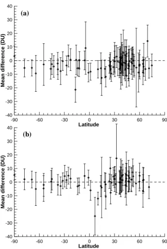
Fig. 1. Means (diamonds) and 1σ standard deviations (error bars) of the Dobson minus TOMS differences at each Dobson spectropho-tometer station; (a) Dobson-N7T differences (b) Dobson-EPT dif-ferences.
found that the size of the ozone hole using the threshold of O3<220 DU was rather insensitive to changes in effective
equivalent stratospheric chlorine (EESC; Daniel et al., 1995) as discussed in greater detail in Sect. 3.2.
2 Homogenization of the satellite data
The data base used in this analysis is an update and extension of the homogenized total column ozone data set developed by Bodeker et al. (2001a) (hereafter referred to as B2001). Specific changes include:
– Version 8 Nimbus 7 and Earth Probe TOMS (Total
Ozone Mapping Spectrometer) data are used rather than version 7 (http://toms.gsfc.nasa.gov/).
– GOME data from the European Space Agency (ESA)
are updated from version 2.4 (used in B2001) to version 3.1. 1996 1997 1998 1999 2000 2001 2002 2003 Year -20 -15 -10 -5 0 5 10 15 20 25 D o b s o n E a rt h P ro b e T O M S ( D U ) 90oS to 60oS 60oS to 30oS 30o S to 0o S 0oN to 30oN 30oN to 60oN 60oN to 90oN
Fig. 2. Mean Dobson-EPT differences for each year and for a range of latitude zones (symbols) together with their 1σ standard devia-tions.
– Assimilated total column ozone fields from KNMI
(http://www.knmi.nl/goa) based on GOME measure-ments are included.
– KNMI TOGOMI total column ozone fields (http://
www.temis.nl/protocols/O3total.html) are included.
– Version 8 SBUV (Solar Backscatter Ultra-Violet) data
from the NASA Nimbus 7, NOAA 9, NOAA 11 and NOAA 16 satellites (http://www.cpc.ncep.noaa. gov/products/stratosphere/sbuv2to/) are included. and the analysis period is extended to the end of 2003 (B2001 analyses extended to the end of 1998). The updates to B2001 associated with each of these changes are detailed in Sects. 2.1 to 2.5.
2.1 Change from version 7 to version 8 TOMS ozone Recently the Nimbus 7 TOMS (N7T) and Earth Probe TOMS (EPT) measurements were reprocessed using version 8 of the retrieval algorithm. This algorithm implements a number of improvements over the earlier version 7 algorithm (McPeters et al., 1996). The total column ozone retrievals are improved for conditions such as high tropospheric aerosol loading, sun glint, persistent snow/ice, and very high solar zenith angles (Wellemeyer et al., 2004). Use of a vertical ozone profile climatology dependent on latitude and season reduces errors due to limited sensitivity of backscattered ultraviolet radi-ance to ozone in the lower troposphere. The algorithm also includes an improved cloud height database from the Nimbus 7 Temperature Humidity Infrared Radiometer (THIR) and a more accurate terrain height data base (Wellemeyer et al., 2004; Labow et al., 2004).
Three-hourly means of version 8 N7T and EPT overpass data and direct-sun only Dobson spectrophotometer mea-surements were calculated at all Dobson spectrophotometer
1979 1981 1983 1985 1987 1989 1991 1993 Year -90 -75 -60 -45 -30 -15 0 15 30 45 60 75 90 L a ti tu d e 1997 1999 2001 2003 Year -90 -75 -60 -45 -30 -15 0 15 30 45 60 75 90
Nimbus-7
Earth Probe
-20 -16 -12 -8 -4 0 4 8 12 16 20
Dobson - TOMS difference (DU)
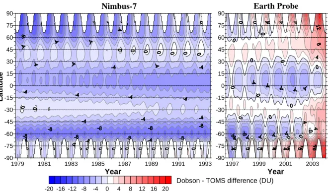
Fig. 3. The fit to the Dobson-N7T differences (Dobson minus TOMS) and the Dobson-EPT differences. Contour intervals are 2 DU. Regions with positive differences are shown in red (TOMS underestimates ozone) while regions with negative differences are shown in blue (TOMS overestimates ozone). Masked areas in winter high latitudes indicate where comparisons cannot be made since these regions are in polar night were no measurements can be made.
sites submitting data to the World Ozone and Ultraviolet Ra-diation Data Centre (WOUDC). The acceptance criteria for the Dobson measurements were tightened over those em-ployed in B2001 so that only “AD wavelength, ordinary setting” (WlCode=0) and direct sun (ObsCode=0) measure-ments were used. As a result, Longyear, Uccle, and Sofia were no longer used in the comparisons with N7T and Ny Alesund, Sofia, and Salto were no longer used in the compar-isons with EPT (cf. Table 2 of B2001). Additional sites used in the EPT intercomparison were Moscow, Lisbon (also for N7T), and Ushuaia. An updated version of Fig. 1 of B2001 is shown in Fig. 1 here.
In comparison to the differences shown in B2001, the dif-ferences shown in Fig. 1 are significantly smaller showing a dramatic improvement in the version 8 TOMS data over the version 7 data when compared with Dobson spectrophotome-ter measurements. More recently, however, an anomaly in the EPT data has been discovered (McPeters, personal com-munication) evident as increasing differences between EPT and coincident Dobson measurements from 2002 onwards (Fig. 2).
To incorporate the increasing drift between the EPT and Dobson measurements in recent years, an additional linear trend term, set to zero before 2002, was added to the 22 pa-rameter function fit to the Dobson-TOMS differences used in B2001. Such functions are fitted to the difference data
sets to avoid the effects of local inhomogeneities in the Dob-son time series, different temporal distribution of the DobDob-son data, and different geographical coverage of the Dobson data. The resultant function fits are shown in Fig. 3.
An increased trend in the Dobson-EPT differences beyond 2002 is clear in the right hand panel of Fig. 3. The additional trend in the differences beyond 2002 is 3.33 DU/year. Be-fore 2002, and over the majority of the globe, the differences between the version 8 N7T and EPT data and measurements from the global Dobson spectrophotometer network are less than 10 DU and show little or no drift. As in B2001, the function fits plotted in Fig. 3 were applied as corrections to the N7T and EPT data, though in this case the corrections applied are much smaller than the corrections applied to the version 7 data.
To correct for any potential offset and drift between the corrected version 8 TOMS data and the version 7 Meteor 3 TOMS (M3T) and Adeos TOMS (ADT) data, daily 2◦zonal
means for each data set were calculated and differenced dur-ing their period of overlap (for M3T: 22 August 1991 to 6 May 1993; for ADT: 11 September 1996 to 29 June 1997). For the calculation of the zonal means, and for those of the other data sets presented below, there had to be at least two measurements within each of six 60◦ longitudinal sectors. Because corrections to the version 7 data may need to be ap-plied to periods beyond the period of overlap with the version
1996 1997 1998 1999 2000 2001 2002 2003 Year -90 -60 -30 0 30 60 90 L a ti tu d e -20 -16 -12 -8 -4 0 4 8 12 16 20
EPT - ESA GOME difference (DU)
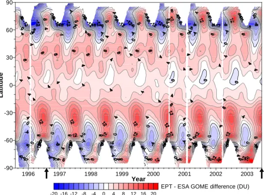
Fig. 4. The fits to the differences between the version 8 EPT zonal means and the ESA GOME zonal means. Contour spacing is 2 DU with the 0 DU contour shown in bold. Regions with positive differences are shown in red (ESA GOME underestimates ozone) while regions with negative differences are shown in blue (ESA GOME overestimates ozone). The arrows on the X axis show the start and end of the period over which the fits were calculated.
8 data (e.g. corrections to M3T beyond 6 May 1993), func-tions of the form
1(φ, t ) = A + B × t + C ×sin(2π t ) + D × cos(2π t)
+E ×sin(4π t) + F × cos(4π t). (1) where 1 is the difference between coincident N7T and M3T or EPT and ADT measurements, and t is the time in deci-mal years, were fitted to the difference time series in each 2◦ zone. At latitudes above 75◦the semi-annual component is not fitted since there is seldom enough data to constrain the fit (as a result of lack of TOMS measurements during polar night). The fits to the differences for M3T and ADT are not shown here but are essentially similar to those reported in B2001.
2.2 Update of ESA GOME data from version 2.4 to 3.1 B2001 used the version 2.4 operational GOME ozone prod-uct from ESA, whereas this study has used updated version 3.1 data. The data are currently available from August 1995 to May 2003. On 22 June 2003 a tape recorder failure on the ERS 2 satellite resulted in only a small portion of the Northern Hemisphere being sampled by the GOME instru-ment thereafter. The fits to the differences between the cor-rected zonal mean EPT data and the ESA GOME data (Eq. 1) are shown in Fig. 4.
Except for the winter-time over southern midlatitudes and winter-time over northern high latitudes, differences are most often less than 10 DU. These difference fits were then used to correct all ESA GOME data.
2.3 KNMI GOME assimilated ozone
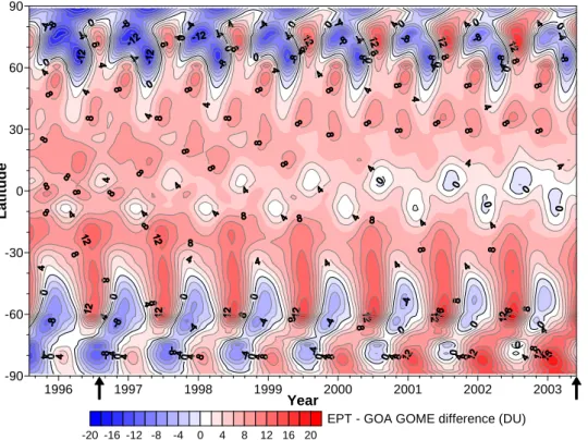
A detailed description of the KNMI assimilated GOME prod-uct (hereafter referred to as GOA) is provided in Eskes et al. (2003). The assimilation is based on the version 3 GOME data processor discussed in the previous section. Synoptic global total column ozone fields are provided every 6 h at 1.5◦ resolution in longitude by 1.0◦ resolution in latitude. As for the ESA GOME product, data are currently available from August 1995 to May 2003. A similar approached to that used to derive corrections to the ESA GOME data was used to derive corrections for the GOA data. The resultant fit of Eq. (1) to the EPT-GOA differences is shown in Fig. 5.
Differences are generally less than 10 DU. When compar-ing Fig. 4 and Fig. 5 it should be kept in mind that since the assimilation is built on an atmospheric transport model, bi-ases in ozone over e.g. middle to high latitudes can be trans-ported to lower latitudes. Furthermore any shortcomings in the transport model such as inadequate representation of the subtropical barrier to transport will be reflected in ozone bi-ases. Finally, any changes in the meteorological reanalyses
1996 1997 1998 1999 2000 2001 2002 2003 Year -90 -60 -30 0 30 60 90 L a ti tu d e -20 -16 -12 -8 -4 0 4 8 12 16 20
EPT - GOA GOME difference (DU)
Fig. 5. The fits to the differences between the corrected version 8 EPT zonal means and the GOA GOME zonal means. Contour spacing is 2 DU with the 0 DU contour shown in bold. Regions with positive differences are shown in red (GOA GOME underestimates ozone) while regions with negative differences are shown in blue (GOA GOME overestimates ozone). The arrows on the X axis show the start and end of the period over which the fits were calculated.
used to drive the model (for the GOA assimilation a change was made from ERA-40 to operational ECMWF analyses in November 1999) may also affect the ozone fields.
2.4 KNMI TOGOMI ozone
A new algorithm for total column ozone retrieval from the GOME instrument has been developed (Valks and van Oss, 2003). This algorithm, named TOGOMI (Total Ozone al-gorithm for GOME using the OMI alal-gorithm), is based on the total ozone Differential Optical Absorption Spec-troscopy (DOAS) algorithm developed for the OMI instru-ment (Veefkind and de Haan , 2001). It resolves various lim-itations of the current operational GOME algorithm (GDP v3) used to generate the ESA GOME data used in this study (Sect. 2.2). A description of some of these limitations was provided in B2001. The main improvements of the new al-gorithm are:
1. New treatment of rotational Raman scattering in the DOAS algorithm. The new formulation explicitly ac-counts for smearing of solar Fraunhofer lines as well as atmospheric tracer absorption structures,
2. Improvements in the calculation of the air mass factor using the so-called empirical approach,
3. A-priori profiles required in the retrieval are taken from the improved ozone profile climatology used in the ver-sion 8 TOMS algorithm (Labow et al., 2004),
4. Using the Fast Retrieval Scheme for Clouds from the Oxygen A-band (FRESCO) algorithm for the cloud cor-rection,
5. Treatment of the atmospheric temperature sensitivity using effective ozone cross-sections calculated from ECMWF temperature profiles,
6. Accurate semi-spherical polarization-dependent radia-tive transfer calculation (KNMI DAK model).
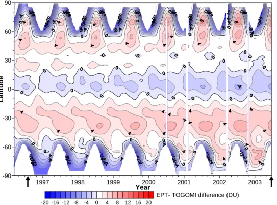
Global total column ozone data fields retrieved using the TOGOMI algorithm are available from 13 March 1996 to 11 August 2003, although for reasons outlined above, only limited data are available from 22 June 2003 onward. The results of the fits of Eq. (1) to differences between TOGOMI and corrected version 8 EPT total column ozone are shown in Fig. 6.
Over most of the globe between 60◦N and 60◦S, the differences are less than 10 DU. Differences become larger close to polar night i.e. when the SZA becomes large.
1997 1998 1999 2000 2001 2002 2003 Year -90 -60 -30 0 30 60 90 L a ti tu d e -20 -16 -12 -8 -4 0 4 8 12 16 20
EPT- TOGOMI difference (DU)
Fig. 6. The fits to the differences between the corrected version 8 EPT zonal means and the TOGOMI GOME zonal means. Contour spacing is 2 DU with the 0 DU contour shown in bold. Regions with positive differences are shown in red (TOGOMI underestimates ozone) while regions with negative differences are shown in blue (TOGOMI overestimates ozone). The arrows on the X axis show the start and end of the period over which the fits were calculated.
2.5 SBUV ozone
The four different SBUV data sets used in this analysis are summarized in Table 1.
Data quality control criteria applied to the SBUV total col-umn ozone data included having at least 100 measurements within a hemisphere for the hemisphere of data to be consid-ered valid (see Sect. 3.1 for the process used to fill missing data), data from both ascending and descending orbits were used but with the criterion of SZA<84◦and the data having a maximum residual quality control parameter (ResQC) of 0.2. Data were included where the data quality control flags in the SBUV data files were 0, 10, 100 or 110. This selection was made to maximize data availability without inclusion of poor quality data. In some cases this resulted in shorter time periods of data being available than those listed in Table 1.
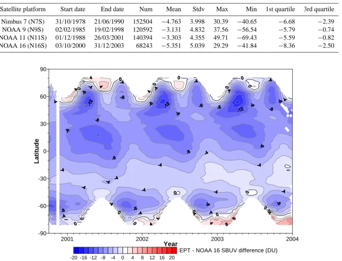
A statistical summary of the differences between the 2◦
zonal means of the 4 SBUV data sets and the corrected ver-sion 8 TOMS data (Nimbus 7 and Earth Probe) is presented in Table 1. The ‘Num’ column shows the number of inter-comparison pairs used to generate the statistics shown in the other columns. For the SBUV instruments on NOAA 9 and NOAA 11, the mean differences are not statistically signifi-cantly different from zero (at the 1σ level). Differences be-tween the corrected TOMS and Nimbus 7/NOAA 16 SBUV
data are somewhat larger. As an example, the function fits (Eq. 1) to the EPT - NOAA 16 SBUV differences are shown in Fig. 7.
Function fits similar to those shown in Fig. 7, derived for all four SBUV data sets, were then used to correct the SBUV data before they were used in the analyses presented below.
3 Antarctic ozone depletion indices
3.1 Data selection and missing data
The 11 data sets described above are corrected using their relevant correction functions and then combined to form a single homogeneous data set spanning the period Novem-ber 1978 to DecemNovem-ber 2003. For each day, a single source of data is selected with the order of priority being (highest to lowest): Nimbus 7 TOMS, Earth Probe TOMS, Meteor 3 TOMS, Adeos TOMS, GOA GOME, TOGOMI GOME, ESA GOME, Nimbus 7 SBUV, NOAA 9 SBUV, NOAA 11 SBUV and finally NOAA 16 SBUV. It was felt that the su-perior spatial coverage and small TOMS-GOA differences made the GOA data preferable to the two other GOME data sets. The sparsity of the SBUV measurements places them at lowest priority.
Table 1. The SBUV data used in this study together with a summary of TOMS (corrected N7T and EPT) - SBUV differences (TOMS minus SBUV). Difference values are in DU.
Satellite platform Start date End date Num Mean Stdv Max Min 1st quartile 3rd quartile Nimbus 7 (N7S) 31/10/1978 21/06/1990 152504 −4.763 3.998 30.39 −40.65 −6.68 −2.39 NOAA 9 (N9S) 02/02/1985 19/02/1998 120592 −3.131 4.832 37.56 −56.54 −5.79 −0.74 NOAA 11 (N11S) 01/12/1988 26/03/2001 140394 −3.303 4.355 49.71 −69.43 −5.59 −0.82 NOAA 16 (N16S) 03/10/2000 31/12/2003 68243 −5.351 5.039 29.29 −41.84 −8.36 −2.50 2001 2002 2003 2004 Year -90 -60 -30 0 30 60 90 L a ti tu d e -20 -16 -12 -8 -4 0 4 8 12 16 20
EPT - NOAA 16 SBUV difference (DU)
Fig. 7. The fits to the differences between the version 8 EPT zonal means and the NOAA 16 SBUV zonal means. Contour spacing is 2 DU with the 0 DU contour shown in bold. Regions with positive differences are shown in red (SBUV underestimates ozone) while regions with negative differences are shown in blue (SBUV overestimates ozone).
For many of the indices presented below, total column ozone values within the region of polar night need to be es-timated. In this study the ‘over the pole’ linear interpolation method described and validated in Bodeker et al. (2001b) was used with the following constraints: interpolation in the zonal direction was not performed over more than 60◦, inter-polation in the meridional direction was not performed over more than 10◦(this constraint was relaxed poleward of 60◦S to allow linear interpolation over the polar cap), and follow-ing the interpolation within these constraints there had to be no missing data poleward of 40◦S. If any of these constraints could not be met, the data set for that day was rejected.
The relative priority of the Earth Probe TOMS and GOA GOME data sets is debatable. While the GOA GOME data provide coverage during the polar night and therefore require no interpolation of missing data, they are essentially model output and may be influenced by shortcomings in the un-derlying transport model (Sect. 2.3). Then again, the ozone column forecast uncertainty generated along with the GOA GOME data could be used to screen for values that are “far away” from the measurements being assimilated. To test whether such a change in priority would affect the results, a second analysis was performed with the GOA GOME data placed higher in priority than the Earth Probe TOMS data. Where these results differ from those presented below, the differences are discussed.
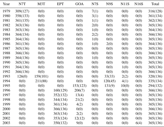
In this analysis, only southern hemisphere ozone fields are used. The number of days of data used from each of the 11 data sets for each year is listed in Table 2.
Table 2. A summary of the data used in this study. The first value shows the number of days of data in the given year from a particular data source. The values in parentheses show the number of days of data from each data source just for the Antarctic Vortex Period (AVP; day 200 to day 335 of each year). Note that in this analysis, no data from ADT, TOGOMI GOME or ESA GOME were used.
Year N7T M3T EPT GOA N7S N9S N11S N16S Total
1979 309(127) 0(0) 0(0) 0(0) 7(1) 0(0) 0(0) 0(0) 316(128) 1980 358(133) 0(0) 0(0) 0(0) 3(1) 0(0) 0(0) 0(0) 361(134) 1981 361(135) 0(0) 0(0) 0(0) 1(1) 0(0) 0(0) 0(0) 362(136) 1982 363(136) 0(0) 0(0) 0(0) 2(0) 0(0) 0(0) 0(0) 365(136) 1983 363(136) 0(0) 0(0) 0(0) 1(0) 0(0) 0(0) 0(0) 364(136) 1984 364(134) 0(0) 0(0) 0(0) 2(2) 0(0) 0(0) 0(0) 366(136) 1985 364(136) 0(0) 0(0) 0(0) 1(0) 0(0) 0(0) 0(0) 365(136) 1986 361(136) 0(0) 0(0) 0(0) 1(0) 2(0) 0(0) 0(0) 364(136) 1987 365(136) 0(0) 0(0) 0(0) 0(0) 0(0) 0(0) 0(0) 365(136) 1988 366(136) 0(0) 0(0) 0(0) 0(0) 0(0) 0(0) 0(0) 366(136) 1989 364(136) 0(0) 0(0) 0(0) 1(0) 0(0) 0(0) 0(0) 365(136) 1990 365(136) 0(0) 0(0) 0(0) 0(0) 0(0) 0(0) 0(0) 365(136) 1991 364(136) 0(0) 0(0) 0(0) 0(0) 0(0) 1(0) 0(0) 365(136) 1992 366(136) 0(0) 0(0) 0(0) 0(0) 0(0) 0(0) 0(0) 366(136) 1993 126(0) 159(101) 0(0) 0(0) 0(0) 33(33) 2(2) 0(0) 320(136) 1994 0(0) 211(88) 0(0) 0(0) 0(0) 120(45) 4(1) 0(0) 335(134) 1995 0(0) 0(0) 0(0) 153(123) 0(0) 131(9) 10(0) 0(0) 294(132) 1996 0(0) 0(0) 160(129) 206(7) 0(0) 0(0) 0(0) 0(0) 366(136) 1997 0(0) 0(0) 352(132) 13(4) 0(0) 0(0) 0(0) 0(0) 365(136) 1998 0(0) 0(0) 344(134) 21(2) 0(0) 0(0) 0(0) 0(0) 365(136) 1999 0(0) 0(0) 361(134) 4(2) 0(0) 0(0) 0(0) 0(0) 365(136) 2000 0(0) 0(0) 366(136) 0(0) 0(0) 0(0) 0(0) 0(0) 366(136) 2001 0(0) 0(0) 363(134) 2(2) 0(0) 0(0) 0(0) 0(0) 365(136) 2002 0(0) 0(0) 353(124) 12(12) 0(0) 0(0) 0(0) 0(0) 365(136) 2003 0(0) 0(0) 350(132) 9(0) 0(0) 0(0) 0(0) 6(4) 365(136)
For the calculation of indices over the Antarctic Vortex Pe-riod (AVP; day 200 to day 335), missing values were filled by linear interpolation (interpolated values were zero or close to zero).
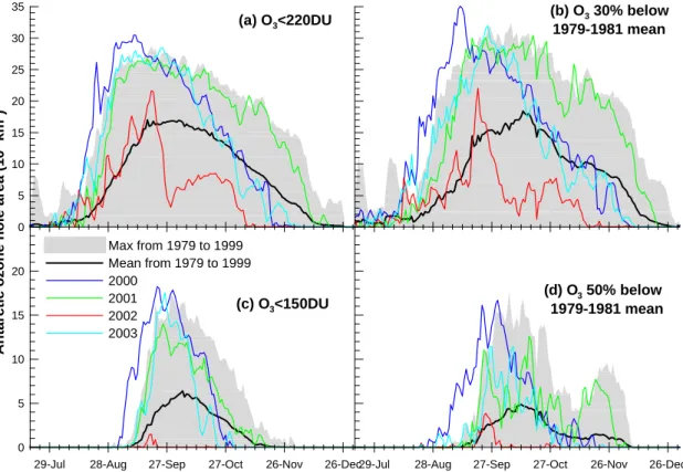
3.2 Antarctic ozone hole area
Daily measures of the area of the Antarctic ozone hole are shown in Fig. 8.
The very weak ozone hole during 2002 is clear, show-ing dramatic reductions in area in late September. For the threshold of O350% below the 1979–1981 mean, there is a
local minimum in the climatology and in the 2001 time se-ries around the second week of November. This may result from the 1979–1981 baseline against which the comparisons are made having atypical seasonal variations during Novem-ber (although the feature persisted if the climatology was ex-tended to 1983). Except for 2001, ozone hole areas during the month of November are close to or lower than the mean values over 1979–1999 suggesting that ozone hole area dur-ing November may be a candidate indicator for Antarctic ozone hole recovery as also observed by Alvarez-Madrigal et al. (2005). This is shown more clearly in Fig. 9 where the
November means of the Antarctic ozone hole area are plotted for each year and for each threshold.
Recent November average ozone hole areas are more sim-ilar to those in the late 1980s or early 1990s. Whether or not the decreases in November average hole areas in the last four years is statistically significant (e.g. applying the methodol-ogy of Reinsel et al. (2002)) is beyond the scope of this paper. Note also the change in periodicity from ∼2 year periodicity up to 1988, 3 year periodicity from 1988 to 2000, and then 2 year periodicity following 2000.
Annual maximum ozone hole areas, and the dates on which they occur, are shown for all four threshold conditions in Fig. 10.
The maximum ozone hole area increases steadily over the 25 year period showing slightly higher values that those derived by Uchino et al. (1999) as a result of the nega-tive offset corrections applied to the satellite-based measure-ments. If the data from the anomalous Antarctic ozone hole in 2002 are ignored, there is little or no indication of a re-duction in the size of the ozone hole using the thresholds of O3<220 DU, O3<150 DU or O330% below the 1979–1981
mean, in agreement with previous studies (Newman et al., 2004). There is some indication however that the area of the
0 5 10 15 20 25 30 35 A n ta rc ti c o z o n e h o le a re a ( 1 0 6 k m 2) 0 5 10 15 20
29-Jul 28-Aug 27-Sep 27-Oct 26-Nov 26-Dec29-Jul 28-Aug 27-Sep 27-Oct 26-Nov 26-Dec
Max from 1979 to 1999 Mean from 1979 to 1999 2000 2001 2002 2003 (a) O3<220DU (b) O3 30% below 1979-1981 mean (c) O3<150DU (d) O3 50% below 1979-1981 mean
Fig. 8. Daily measures of the size of the Antarctic ozone hole using four different criteria. Values for 2000 (blue), 2001 (green), 2002 (red) and 2003 (cyan) are compared against the range of values over the period 1979–1999 (greyed area). The mean ozone hole area over the period 1979 to 1999 is shown using a thick black line in all 4 panels.
1980 1982 1984 1986 1988 1990 1992 1994 1996 1998 2000 2002 Year 0 5 10 15 20 25 N o v e m b e r m e a n A n ta rc ti c o z o n e h o le a re a ( 1 0 6 k m 2) O3<150DU O3<220DU O3 30% below 1979-1981 mean O3 50% below 1979-1981 mean
Fig. 9. November means of the Antarctic ozone hole area for the four different threshold conditions.
ozone hole with ozone 50% below the 1979–1981 mean has decreased; over the 5 year period from 1999 to 2003, except for one year (2000), the area for every year has been below the minimum value over the 5 year period from 1994 to 1998. There is an indication in the bottom panel of Fig. 10 that the date when the maximum occurs has shifted earlier over
0 10 20 30 40 A n ta rc ti c o z o n e h o le a re a ( 1 0 6k m 2) 27-Aug 16-Sep 6-Oct 26-Oct 15-Nov 1978 1980 1982 1984 1986 1988 1990 1992 1994 1996 1998 2000 2002 Year O3<150DU O3<220DU O3 30% below 1979-1981 mean O3 50% below 1979-1981 mean
Date when maximum area occurs
Fig. 10. The annual maximum ozone hole area for the four different threshold conditions, and the dates on which those maxima were achieved.
the period. For the O3<220 DU threshold condition, over
the period 1980 to 2000, the date on which the maximum ozone hole area occurs shifts earlier by more than 2 weeks per decade. For this threshold condition, over the most re-cent 4 years, the maximum area date drifts later by ∼18 days.
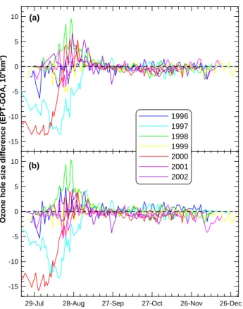
-15 -10 -5 0 5 10 -15 -10 -5 0 5 10 O z o n e h o le s iz e d if fe re n c e ( E P T -G O A , 1 0 6k m 2)
29-Jul 28-Aug 27-Sep 27-Oct 26-Nov 26-Dec
1996 1997 1998 1999 2000 2001 2002 (a) (b)
Fig. 11. Differences in the size of the Antarctic ozone hole calcu-lated using the Earth Probe TOMS and GOA GOME data sets (EPT-GOA) for (a) corrected EPT and GOA data, (b) corrected EPT and uncorrected GOA data.
Again, whether or not this is a sign of statistically significant ozone recovery is beyond the scope of the paper.
Early in the season there are differences in the size of the ozone hole calculated using the Earth Probe TOMS and GOA GOME data sets (Fig. 11).
However, because negative corrections were applied to the GOA GOME data over high southern latitudes during winter (Fig. 5) this may result in excessively large ozone hole val-ues. Therefore a comparison of ozone hole areas from the corrected Earth Probe TOMS and uncorrected GOA GOME data sets is also shown in Fig. 11. Except for 1997, 1998 and 2000, the differences are generally less than 5 million km2 and after the first week of September are generally less than 2 million km2. The sources of these discrepancies are cur-rently unknown but most likely relate to how the GOA as-similation model uses measurements close to the vortex edge (which may be in sunlight and therefore subject to ozone de-pletion chemistry) to infer ozone values deep within the vor-tex. In any event, the differences do not affect the results shown in Fig. 9 and Fig. 10.
1978 1980 1982 1984 1986 1988 1990 1992 1994 1996 1998 2000 2002 Year 12-Aug 26-Aug 9-Sep 23-Sep 7-Oct 21-Oct 4-Nov 18-Nov 2-Dec 16-Dec 30-Dec D a te o f d is a p p e a ra n c e o f o z o n e h o le o z o n e v a lu e s O3<150DU O3<220DU O3 30% below 1979-1981 mean O3 50% below 1979-1981 mean
Fig. 12. The annual dates of disappearance of ozone hole type val-ues for all four threshold criteria. In 1988 there were no ozone values below 150 DU.
3.3 Date of ozone hole disappearance
The annual dates of disappearance of ozone levels flagged as ozone hole values (latitude ≥40◦S) for all four threshold criteria are shown in Fig. 12.
The dates of disappearance of ozone hole values drift later into the year up until 1998/1999. Thereafter the date has shifted earlier in the year for all four threshold criteria. To investigate whether the recent earlier dates of disappearance of vortex like values are related to changes in the timing of the breakdown of the dynamical vortex, meridional impermi-ability, κ, on the 450 K surface was calculated for each day of each year (Bodeker et al., 2002). The date on which the meridional maximum κ value falls below 10% of its annual maximum value was used to denote the dissipation of the dynamical vortex. Previous analyses have shown that from the late 1970s to the late 1990s the date of breakdown of the dynamical vortex has drifted later in the year by between 2 and 4 weeks, depending on the metric used to detect vortex breakdown (Uchino et al., 1999; Waugh et al., 1999). In 2000 and 2002 the dynamical vortex dissipated on the 19 and 18 November respectively (not shown graphically here). This was earlier than any previous vortex breakdown since 1979 when the vortex also dissipated on 18 November. In 2001, although the vortex dissipated on 14 December, 1 day later than in 1999, ozone hole like values disappeared 12 days ear-lier in 2001 than in 1999 suggesting that mechanisms other than changes in dynamics may also be driving earlier disap-pearance of ozone levels typical of the Antarctic ozone hole. In 2003 the dynamical vortex dissipated on 30 November which is also relatively early compared to the 1990s where in only two years (27 November 1991; 30 November 1997) did the vortex dissipate in November.
Earlier dates of dissipation of the dynamical vortex, and earlier dates of disappearance of ozone hole ozone values,
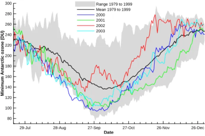
29-Jul 28-Aug 27-Sep 27-Oct 26-Nov 26-Dec Date 80 100 120 140 160 180 200 220 240 260 280 300 M in im u m A n ta rc ti c o z o n e ( D U ) Range 1979 to 1999 Mean 1979 to 1999 2000 2001 2002 2003
Fig. 13. Minimum Antarctic ozone levels for 2000 (blue), 2001 (green), 2002 (red) and 2003 (cyan) compared against the 1979-1999 climatology (range shown in grey and mean shown with thick black line).
have important implications for summer-time UV levels over southern midlatitudes (McKenzie et al., 1999). The closer the date of dissipation of the vortex to the summer solstice, the greater the likelihood of ozone depleted fragments of the vortex being advected to midlatitudes at times when the UV is high.
3.4 Daily minimum ozone levels
Daily minimum ozone levels south of 40◦S have been calcu-lated for each day from the assimicalcu-lated total column ozone data base. A comparison of these values for 2000 to 2003 against the 1979 to 1999 climatology is presented in Fig. 13. The minimum Antarctic ozone levels for the year 2000 to 2003 are generally close to the lower range of the 1979 to 1999 climatology up until the end of September. Dur-ing November however, the values are more typical of the mean of the 1979 to 1999 climatology. As already reported by Alvarez-Madrigal et al. (2005), this suggests that min-imum ozone levels over Antarctic in November are show-ing a more immediate return to pre-ozone hole values than the minimum values in September. When GOA GOME data are used in preference to Earth Probe TOMS data, minimum ozone values over the Antarctic in 2000 (where the differ-ences are largest c.f. Fig. 11) are 20–40 DU lower than those shown in Fig. 13 but become very close to those shown in Fig. 13 by mid-August.
Annual minimum ozone levels south of 40◦S together with the dates on which the minimum values occurred are plotted in Fig. 14.
While the annual minimum Antarctic total column ozone levels over recent years appear to show an up turn, the date on which the annual minimum occurs appears to continue moving earlier into the year over the whole analysis period.
80 100 120 140 160 180 200 M in im u m A n ta rc ti c o z o n e ( D U ) 16-Sep 26-Sep 6-Oct 16-Oct 26-Oct 5-Nov 1978 1980 1982 1984 1986 1988 1990 1992 1994 1996 1998 2000 2002 Year
Date when Min ozone occurs
Fig. 14. Annual minimum Antarctic total column ozone levels and the date on which these minimum values occurred.
1978 1980 1982 1984 1986 1988 1990 1992 1994 1996 1998 2000 2002 2004 Year 0 2 4 6 8 10 12 14 16 18 V o rt e x p e ri o d ( 1 9 J u ly 1 D e c e m b e r) a v e ra g e d a il y o z o n e d e fi c it o v e r A n ta rc ti c a ( m il li o n t o n s )
Using corrected EPT Using uncorrected EPT
Fig. 15. The AVP mean ozone mass deficit (O3<220 DU) for each
year in 109kg. Values derived using the EPT data corrected af-ter comparison with Dobson spectrophotomeaf-ter measurements are shown using diamonds, while values derived using uncorrected EPT data are shown using circles.
The results are unaffected by the relative priority of the EPT and GOA data sets.
3.5 Ozone mass deficit
As in Bodeker and Scourfield (1995), the AVP mean ozone mass deficit has been calculated for each year and is plotted in Fig. 15.
The mass deficit provides a direct measure of the mass of ozone that would need to be added to the atmosphere to re-turn ozone values over the Antarctic to above 220 DU and aids comparison with ozone changes over other parts of the globe (Uchino et al., 1999; Bodeker et al., 2001b). Clearly the application of the small corrections to the EPT data can change the conclusions that may be drawn from the ozone mass deficit data on recovery of the Antarctic ozone hole. Unlike the annual maximum area and the annual minimum
total column ozone which show little change through the 1990s, the ozone mass deficit shows significant growth dur-ing the 1990s, almost doubldur-ing in value from 8.6×10⁹kg in 1990 to 15.2×10⁹kg in 2000. This results from more severe depletion occurring close to the vortex edge (Bodeker et al., 2002; Newman et al., 2004) which changes the shape of the vortex (more bucket shaped rather than funnel shaped) with-out significantly changing the area of the ozone hole or the minimum values within the hole. Therefore, use of ozone hole area or minimum ozone values may not be the best met-rics to gauge changes in the severity of the Antarctic ozone hole in recent years. These results are also unaffected by the relative priority of the EPT and GOA data sets.
4 Conclusions
A number of metrics describing the evolution of the Antarc-tic ozone hole over the period 1979 to 2003 have been devel-oped. While some indicators such as the annual maximum ozone hole area and annual minimum ozone over the Antarc-tic show signs of saturation over the 1990s and the first few years of this century, the AVP mean ozone mass deficit shows large increases over the 1990s and clear signs of decreases over the period 1998 to 2003 (as long as the necessary cor-rections are applied to the Earth Probe TOMS data to account for their increasing drift with respect to the ground-based Dobson spectrophotometer network). This analysis therefore suggests that indicators such as the AVP mean ozone mass deficit, the annual date of disappearance of ozone hole val-ues, or the November means of the Antarctic ozone hole area may be more suitable indicators for detecting the recovery of the Antarctic ozone hole than e.g. the annual maximum area of the hole or the annual minimum ozone values over the Antarctic. Whether or not they will ultimately be useful as indicators of Antarctic ozone hole recovery relies on the additional step of attributing the observed changes in the in-dicators to changes in ozone depleting substances. This is beyond the current scope of this paper. Many of the indica-tors derived above show a change in behaviour in the past 4 or 5 years. Whether or not this change is indicative of the onset of recovery in the Antarctic ozone hole is not yet clear and requires more detailed statistical investigation.
Acknowledgements. We would like to thank the Laboratory for
Atmospheres at GSFC for access to SBUV and TOMS data, ESA/ESRIN for access to GOME data, NOAA for access to the SBUV data from the NOAA 9, NOAA 11 and NOAA 16 satel-lites, and Chi-Fan Shih at the National Center for Atmospheric Re-search and the National Centers for Environmental Prediction for the NCEP/NCAR data. We acknowledge Pieter Valks (DLR) who was involved in the development of TOGOMI, and Ronald van der A who processed the TOGOMI data set. We would also like to that the WOUDC for providing total column ozone measurements from the Dobson spectrophotometer network. This work was conducted within the FRST funded Drivers and Mitigation of Global Change programme (C01X0204).
Edited by: M. Dameris
References
Alvarez-Madrigal, M. and P´erez-Peraza, J.: Analysis of the evo-lution of the Antarctic ozone hole size, J. Geophys. Res., 110, D02107, doi:10.1029/2004JD004944, 2005.
Austin, J., Shindell, D., Beagley, S. R., Br¨uhl, C., Dameris, M., Manzini, E., Nagashima, T., Newman, P., Pawson, S., Pitari, G., Rozanov, E., Schnadt, C., and Shepherd, T. G.: Uncertainties and assessments of chemistry-climate models of the stratosphere, Atmos. Chem. Phys., 3, 1–27, 2003,
SRef-ID: 1680-7324/acp/2003-3-1.
Bodeker, G. E. and Scourfield, M. W. J.: Planetary waves in total ozone and their relation to Antarctic ozone depletion, Geophys. Res. Lett., 22(21), 2949–2952, 1995.
Bodeker, G., Scott, J., Kreher, K., and McKenzie, R.: Global ozone trends in potential vorticity coordinates using TOMS and GOME intercompared against the Dobson network: 1978–1998, J. Geo-phys. Res., 106, 23 029–23 042, 2001a.
Bodeker, G. E., Connor, B. J., Liley, J. B., and Matthews, W. A.: The global mass of ozone: 1978–1998, Geophys. Res. Lett., 28(14), 2819–2822, 2001b.
Bodeker, G. E., Struthers, H., and Connor, B. J.: Dynamical containment of Antarctic ozone depletion, Geophys. Res. Lett., 29(7), doi:10.1029/2001GL014206, 2002.
Daniel, J. S., Solomon, S., and Albritton, D. L.: On the evaluation of halocarbon radiative forcing and global warming potentials, J. Geophys. Res., 100(D1), 1271–1285, 1995.
Eskes, H. J.,van Velthoven, P. F. J., Valks, P. J. M., and Kelder, H. M.: Assimilation of GOME total ozone satellite observations in a three-dimensional tracer transport model, Q. J. R. Meteorol. Soc., 129, 1663–1681, 2003.
Fioletov, V. E., Bodeker, G. E., Miller, A. J., McPeters, R. D., and Stolarski, R.: Global and zonal total ozone variations estimated from ground-based and satellite measurements: 1964–2000, J. Geophys. Res., 107(D22), 4647, doi:4610.1029/2001JD001350, 2002.
Labow, G. J., McPeters, R. D., and Bhartia, P. K.: A compari-son of TOMS & SBUV version 8 total column ozone data with data from groundstations, in: Ozone, Proceedings of the XX Quadrennial Ozone Symposium, 1—8 June 2004, Kos, Greece, Vol. 1, edited by: Zerefos, C. S., pp. 123–124, International Ozone Commission, Athens, Greece, 2004.
McKenzie, R., Connor, B., and Bodeker, G.: Increased summertime UV radiation in New Zealand in response to ozone loss, Science, 285, 1709–1711, 1999.
McPeters, R. D., Bhartia, P. K., Krueger, A. J., Herman, J. R., Schlesinger, B. M., Wellemeyer, C. G., Seftor, C. J., Jaross, G., Taylor, S. L., Swissler, T., Torres, O., Labow, G., Byerly, W., and Cebula, R. P.: Nimbus-7 Total Ozone Mapping Spectrome-ter (TOMS) data products user’s guide, NASA Ref. Publ. 1384, 1996.
Montzka, S., Butler, J., Myers, R. M. T., Swanson, T., Clarke, A., Lock, L., and Elkins, J.: Decline in the tropospheric abun-dance of halogen from halocarbons: implications for stratopsh-eric ozone depletion, Science, 272, 1318–1320, 1996.
Newman, P. A., Kawa, S. R., and Nash, E. R.: On the size of the Antarctic ozone hole, Geophys. Res. Lett., 31, L21104,
doi:10.1029/2004GL020596, 2004.
Reinsel, G., Weatherhead, E. C., Tiao, G. C., Miller, A. J., Nagatani, R., Wuebbles, D. J., and Flynn, L. E.: On detection of turnaround and recovery in trend for ozone, J. Geophys. Res., 107(D10), doi:10.1029/2001JD000500, 2002.
Rinsland, C. P., Mahieu, E., Zander, R., Jones, N. B., Chipperfield, M. P., Goldman, A., Anderson, J., Russell III, J. M., Demoulin, P., Notholt, J., Toon, G. C., Blavier, J.-F., Sen, B., Sussmann, R., Wood, S. W., Meier, A., Griffith, D. W. T., Chiou, L. S., Murcray, F. J., Stephen, T. M., Hase, F., Mikuteit, S., Schulz, A., and Blumenstock, T.: Long-term trends of inorganic chlo-rine from ground-based infrared solar spectra: Past increases and evidence for stabilization, J. Geophys. Res., 108(D8), 4252, doi:4210.1029/2002JD003001, 2003.
Uchino, O., Bojkov, R., Balis, D.S., Akagi, K., Hayashi, M., and Kajihara, R.: Essential characteristics of the Antarctic-spring ozone decline: update to 1998, Geophys. Res. Lett., 26(10), 1377–1380, 1999.
Valks, P. and van Oss, R.: TOGOMI Algorithm Theoretical Basis Document, KNMI/ESA, 2003.
Veefkind, J. P. and de Haan, J. F.: OMI Algorithm Theoretical Ba-sis Document, DOAS Total Ozone Algorithm, ATBD-OMI-02, Version 1.0, edited by: Bhartia, P. K., Vol. II, 2001.
Waugh, D. W., Randel, W. J., Pawson, S., Newman, P., and Nash, E. R.: Persistence of the lower stratospheric polar vortices, J. Geophys. Res., 104(D22), 27 191–27 201, 1999.
Wellemeyer, C. G., Bhartia, P. K., McPeters, R. D., Taylor, S. L., and Ahn, Ch.: A new release of data from the Total Ozone Mapping Spectrometer (TOMS), SPARC Newletter, 22, 37–38, SparcOffice, Service d’ A´eronomie, Verri`eres-le-Buisson cedex, France, 2004, available at http://www.atmosp.physics.utoronto. ca/SPARC/.
WMO: Scientific Assessment of Ozone Depletion: 2002. Global Ozone Research and Monitoring Project, Report No. 47, World Meteorological Organization, Geneva, 498 pp, 2003.