High-resolution hypernuclear spectroscopy at Jefferson Lab, Hall A

arXiv:1807.09720v2 [nucl-ex] 26 Jul 2018

High-resolution hypernuclear spectroscopy at Jefferson Lab, Hall A

F. Garibaldi,1 _{A. Acha,}2 _{P. Ambrozewicz,}2 _{K.A. Aniol,}3 _{P. Baturin,}4 _{H. Benaoum,}5 _{J. Benesch,}6 P.Y. Bertin,7 _{K.I. Blomqvist,}8 _{W.U. Boeglin,}2 _{H. Breuer,}9 _{P. Brindza,}6 _{P. Bydˇzovsk´y,}10 _{A. Camsonne,}7

C.C. Chang,9 _{J.-P. Chen,}6 _{Seonho Choi,}11 _{E.A. Chudakov,}6 _{E. Cisbani,}12 _{S. Colilli,}12 _{L. Coman,}2 F. Cusanno,1 _{B.J. Craver,}13_{G. De Cataldo,}14 _{C.W. de Jager,}6 _{R. De Leo,}14 _{A.P. Deur,}13 _{C. Ferdi,}7 R.J. Feuerbach,6 _{E. Folts,}6 _{S. Frullani,}1 _{O. Gayou,}15 _{F. Giuliani,}12 _{J. Gomez,}6 _{M. Gricia,}12 _{J.O. Hansen,}6 D. Hayes,16 _{D.W. Higinbotham,}6_{T.K. Holmstrom,}17 _{C.E. Hyde,}16, 7 _{H.F. Ibrahim,}18 _{M. Iodice,}19 _{X. Jiang,}4

L.J. Kaufman,20 _{K. Kino,}21 _{B. Kross,}6 _{L. Lagamba,}14 _{J.J. LeRose,}22 _{R.A. Lindgren,}13 _{M. Lucentini,}12 D.J. Margaziotis,3_{P. Markowitz,}2_{S. Marrone,}14_{D.G. Meekins,}6 _{Z.E. Meziani,}11_{K. McCormick,}4 _{R.W. Michaels,}6

D.J. Millener,23 _{T. Miyoshi,}24 _{B. Moffit,}17 _{P.A. Monaghan,}15 _{M. Moteabbed,}2 _{C. Mu˜noz Camacho,}25 S. Nanda,6 _{E. Nappi,}14 _{V.V. Nelyubin,}13 _{B.E. Norum,}13 _{Y. Okasyasu,}24 _{K.D. Paschke,}20_{C.F. Perdrisat,}17 E. Piasetzky,26 _{V.A. Punjabi,}27 _{Y. Qiang,}15_{B. Raue,}2 _{P.E. Reimer,}28 _{J. Reinhold,}2 _{B. Reitz,}6 _{R.E. Roche,}29

V.M. Rodriguez,30 _{A. Saha,}6 _{F. Santavenere,}12_{A.J. Sarty,}31 _{J. Segal,}6 _{A. Shahinyan,}32 _{J. Singh,}13 S. ˇSirca,33 _{R. Snyder,}13 _{P.H. Solvignon,}11 _{M. Sotona,}10 _{R. Subedi,}34 _{V.A. Sulkosky,}17 _{T. Suzuki,}24 H. Ueno,35 _{P.E. Ulmer,}16 _{G.M. Urciuoli,}36_{E. Voutier,}37 _{B.B. Wojtsekhowski,}6 _{X. Zheng,}28_{and C. Zorn}6

(Jefferson Lab Hall A Collaboration) 1

Istituto Nazionale di Fisica Nucleare, Sezione di Roma, Piazzale A. Moro 2, I-00185 Rome, Italy 2_{Florida International University, Miami, Florida 33199, USA}

3_{California State University, Los Angeles, Los Angeles California 90032, USA} 4_{Rutgers, The State University of New Jersey, Piscataway, New Jersey 08855, USA}

5_{Syracuse University, Syracuse, New York 13244, USA}

6_{Thomas Jefferson National Accelerator Facility, Newport News, Virginia 23606, USA} 7_{Universit´e Blaise Pascal/IN2P3, F-63177 Aubi`ere, France}

8_{Universit¨at Mainz, Mainz, Germany}

9_{University of Maryland, College Park, Maryland 20742, USA} 10_{Nuclear Physics Institute, ˇReˇz near Prague, Czech Republic} 11

Temple University, Philadelphia, Pennsylvania 19122, USA 12_{Istituto Nazionale di Fisica Nucleare, Sezione di Roma,}

gruppo collegato Sanit`a, and Istituto Superiore di Sanit`a, I-00161 Rome, Italy 13_{University of Virginia, Charlottesville, Virginia 22904, USA}

14_{Istituto Nazionale di Fisica Nucleare, Sezione di Bari and University of Bari, I-70126 Bari, Italy} 15_{Massachussets Institute of Technology, Cambridge, Massachusetts 02139, USA}

16_{Old Dominion University, Norfolk, Virginia 23508, USA} 17_{College of William and Mary, Williamsburg, Virginia 23187, USA}

18_{Cairo University, Giza 12613, Egypt}

19_{Istituto Nazionale di Fisica Nucleare, Sezione di Roma Tre, I-00146 Rome, Italy} 20_{University of Massachussets Amherst, Amherst, Massachusetts 01003, USA} 21_{Research Center for Nuclear Physics, Osaka University, Ibaraki, Osaka 567-0047, Japan}

22_{Chesapeake Bay Governor’s School, Tappahannock, Virginia 222560, USA} 23_{Brookhaven National Laboratory, Upton, New York 11973, USA}

24_{Tohoku University, Sendai, 980-8578, Japan}

25_{CEA Saclay, DAPNIA/SPhN, F-91191 Gif-sur-Yvette, France}

26_{School of Physics and Astronomy, Sackler Faculty of Exact Science, Tel Aviv University, Tel Aviv 69978, Israel} 27_{Norfolk State University, Norfolk, Virginia 23504, USA}

28_{Argonne National Laboratory, Argonne, Illinois 60439, USA} 29_{Florida State University, Tallahassee, Florida 32306, USA}

30_{University of Houston, Houston, Texas 77204, USA} 31_{St. Mary’s University, Halifax, Nova Scotia, Canada}

32_{Yerevan Physics Institute, Yerevan, Armenia}

33_{Faculty of Mathematics and Physics, University of Ljubljana, Slovenia} 34_{Kent State University, Kent, Ohio 44242, USA}

35_{Yamagata University, Yamagata 990-8560, Japan}

36_{Istituto Nazionale di Fisica Nucleare, Sezione di Roma, P.zza Aldo Moro 2, Rome, Italy} 37_{LPSC, Universit´e Joseph Fourier, CNRS/IN2P3, INPG, F-38026 Grenoble, France}

(Dated: July 27, 2018)

The experiment E94-107 in Hall A at Jefferson Lab started a systematic study of high resolu-tion hypernuclear spectroscopy in the 0p-shell region of nuclei such as the hypernuclei produced in electroproduction on9_Be,12_{C and}16_{O targets. In order to increase counting rates and provide} un-ambiguous kaon identification two superconducting septum magnets and a ring-imaging ˇCherenkov

detector were added to the Hall A standard equipment. The high-quality beam, the good spec-trometers and the new experimental devices allowed us to obtain very good results. For the first time, measurable strength with sub-MeV energy resolution was observed for the core-excited states of 12

ΛB. A high-quality 16

ΛN hypernuclear spectrum was likewise obtained. A first measurement of the Λ binding energy for16

ΛN, calibrated against the elementary reaction on hydrogen, was obtained with high precision, 13.76 ± 0.16 MeV. Similarly, the first9

ΛLi hypernuclear spectrum shows general agreement with theory (distorted-wave impulse approximation with the SLA and BS3 electropro-duction models and shell-model wave functions). Some disagreement exists with respect to the relative strength of the states making up the first multiplet. A Λ separation energy of 8.36 MeV was obtained, in agreement with previous results. It has been shown that the electroproduction of hypernuclei can provide information complementary to that obtained with hadronic probes and the γ-ray spectroscopy technique.

I. INTRODUCTION

The physics of hypernuclei, multibaryonic systems with non-zero strangeness, is an important branch of con-temporary nuclear physics at low energy (structure, en-ergy spectra and weak decays of hypernuclei) as well as at intermediate energy (production mechanism) [1]. The Λ hypernucleus is a long-lived baryonic system (t = 10−10_s) and provides us with a variety of nuclear phenomena. The hyperon inside an ordinary nucleus is not affected by the Pauli principle and can penetrate deeply inside the nucleus permitting measurements of the system response to the stress imposed on it. The study of its propagation can reveal configurations or states not seen in other ways. The study also gives important insight into the structure of ordinary nuclear matter.

An understanding of baryon-baryon interactions is fundamental in order to understand our world and its evolution. However, our current knowledge is limited at the level of strangeness zero particles (p and n). Hence, studying the nucleon (YN) and hyperon-hyperon (YY) interactions is very important in order to extend our knowledge and seek a unified description of them. Since very limited information can be obtained from elementary hyperon-nucleon scattering, hypernu-clei are unique laboratories for studying the ΛN inter-action [2]. In fact, an effective ΛN interinter-action can be determined from hypernuclear spectra obtained from var-ious reactions and can be used to discriminate between different YN potentials employed to carry out ab initio many-body calculations [3].

Until now a large body of data came from two types of highly complementary hypernuclear spectroscopy tech-niques: reaction based spectroscopy with hadron probes and γ-ray spectroscopy [4]. Reaction spectroscopy, which directly populates hypernuclear states, reveals the level structure in the Λ bound region and can even study ex-cited states between the nucleon emission threshold and the Λ emission threshold. It provides information on Λ hypernuclear structure and the Λ emission threshold. The information on Λ hypernuclear structure and the ΛN interaction is obtained through the determination of the hypernuclear masses, spectra, reaction cross sections, an-gular distributions etc. Moreover, precise measurements of the production cross sections provide information on

the hypernuclear production mechanism and the dynam-ics of the elementary-production reaction. γ-ray spec-troscopy achieves ultra-high resolution (typically a few keV). It is a powerful tool for investigation of the spin dependent part of the ΛN interaction, which requires precise information on the level structure of hypernu-clei. Both these powerful techniques have limitations, first limited energy resolution and small spin-flip ampli-tudes, and second the access only to hypernuclear states below nucleon emission threshold.

Experimental knowledge can be greatly improved using electroproduction of strangeness characterized by large three-momentum transfer (∼ 250 MeV/c), large angu-lar momentum transfer ∆J, and strong spin-flip terms, even at zero production angles [4]. Moreover, the K+_Λ pair production occurs on a proton in contrast to a neu-tron in (K−_{, π}−_{) or (π}+_{, K}+_{) reactions making possible} the study of different hypernuclei and charge-dependent effects from a comparison of mirror hypernuclei (charge-symmetry breaking). The hypernuclear γ-ray measure-ments give extremely high-precision energy-level spac-ings, while the precision of the energy levels given by the (e, e′_K+_{) reaction spectroscopy can potentially be a} few hundreds of keV, which is more than an order of magnitude worse than γ-ray measurement. However, the advantage of being able to simultaneously observe more complete structures, as well as to provide precise abso-lute binding energy is obvious. For transitions with en-ergy larger than 1 MeV, a Ge detector efficiency decreases quickly, and thus statistics becomes a major problem for the current γ-ray spectroscopy program using the Ge de-tector technique.

Even though plans for various new hypernuclear physics studies at other facilities exist, the precision, ac-curate mass spectroscopy from the JLab program has a unique position, in addition to the clearly known com-mon advantages of electro-production (such as the size of momentum transfer allowing large angular momen-tum transfer, extra spin transfer from the virtual pho-ton, converting a proton into a Λ to study neutron-rich hypernuclei).

The E94-107 experiment in Hall A at Jefferson Lab [5] started a systematic study of high-resolution hypernu-clear spectroscopy on p-shell targets, specifically9_{Be [6],} 12_{C [7] and}16_{O [8]. Moreover a study of the elementary}

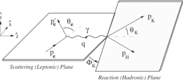
Φ θ_e θ p p' γ q p p H Scattering (Leptonic) Plane

Reaction (Hadronic) Plane

z x y ^ e e K K K ^ ^ 1

FIG. 1. Kinematics of hypernuclear electroproduction in the laboratory frame.

reaction on a proton was performed.

This paper describes the experimental apparatus, the theoretical models, the results obtained and the physics information extracted from them.

II. THE EXPERIMENT

Hall A at Jefferson Lab is well suited to perform (e, e′_K+_{) experiments. Scattered electrons can be} de-tected in the high-resolution spectrometer (HRS) elec-tron arm while coincident kaons are detected in the HRS hadron arm [9]. The disadvantage of smaller electromag-netic cross sections with respect to hadron-induced reac-tions is partially compensated for by the high current, high duty cycle, and high energy resolution capabilities of the beam. The detector packages for the electron and hadron spectrometers are almost identical, except for the particle identification (PID) systems discussed later [9].

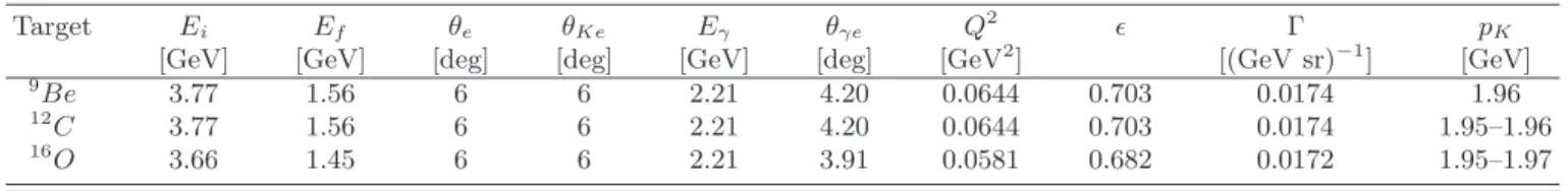
The kinematics for the three experiments is shown in Fig. 1 and values are given in Table I. The beam and fi-nal electron energies are denoted Eiand Ef, respectively, and the electron (θe), kaon (θKe), and photon (θγe) an-gles are measured with respect to the beam direction. The virtual photon energy, transverse polarisation, and flux factor are denoted as Eγ, ǫ, and Γ. The kaon mo-mentum pK changes a little bit due to a different hyper-nucleus mass for the excited states. A coplanar experi-mental setup was chosen with the kaon azimuthal angle ΦK= 180◦. Then the kaon lab angle with respect to the photon direction is θK = θKe− θγe, see Fig. 1.

The reasons for this choice were the following. The momentum transfer to the hypernucleus in the electro-production is rather large (350 MeV/c) and decreases steadily with increasing energy of the virtual photon (Eγ = Ee− Ee′) while the elementary electroproduction cross section, with the kaon detected at forward angles, is almost constant for Eγ=1.2-2.2 GeV. The momentum transfer for forward kaon scattering angles falls from 330 MeV/c at Eγ = 1.2 GeV to 250 MeV/c at Eγ= 2.5 GeV, so that higher energies are preferable. Moreover, because the cross section depends strongly on Q2 _{(through the} virtual photon flux as determined by the electron kine-matics), the measurements have to be made at low Q2_to get reasonable counting rates . Hence, the electron

scat-tering angle must be small, and the kaon angle close to the virtual photon direction in order to minimize the mo-mentum transfer. Moreover, due to the long flight path in the HRS spectrometer, to keep a reasonable kaon sur-vival fraction the kaon momenta must be fairly high.

Good energy resolution together with a low level of background is mandatory for this experiment. The en-ergy resolution depends on the momentum resolution of the HRS spectrometers, on the straggling and energy loss in the target, and on the beam energy spread. A momen-tum resolution of the system (HRS’s + sepmomen-tum magnets) of ∆p/p = 10−4 _{(FWHM) and a beam energy spread as} small as 6 × 10−5 _{(FWHM) are necessary to be able to} get an excitation energy resolution of 700 keV or less. A very good PID system is needed to guarantee a low level of background.

A. The beam

1. Beam monitors

E94-107 desired a continuous wave, 3.66 GeV, 100 µA electron beam with very small energy spread and ver-tical spot size (energy spread σ ≤ 3 × 10−5_{, spot size} σ ≤ 100 µm). With some effort, the CEBAF staff were able to achieve these requirements. The absolute value of the beam energy was measured using the Arc method (see Sec. II A 2). The beamline is segmented into several sections isolated by vacuum valves. The beam diagnos-tic elements consist of transmission-line position itors, current monitors, superharps, viewers, loss mon-itors, and optical transition radiation (OTR) viewers. Drifts in the central beam energy were monitored us-ing the so-called “Hall A Tiefenback Energy” value (see Sec. II A 3). The beam spot size and the energy spread were continuously monitored using a Synchrotron Light Interferometer (SLI) [10] (see Sec. II A 4).

2. The Arc method

The Arc method determines the energy by measur-ing the deflection of the beam in the arc section of the beamline. The nominal bend angle of the beam in the arc section is 34.3◦_{. The measurement is made when the} beam is tuned in dispersive mode in the arc section. The momentum of the beam is then related to the field inte-gral of eight dipoles and the net bend angle through the arc section [9]. The method consists of two simultaneous measurements, one for the magnetic field integral of the bending elements, and one for the actual bend angle of the arc.

TABLE I. Kinematics in the laboratory frame for the three experiments.

Target Ei Ef θe θKe Eγ θγe Q2 ǫ Γ pK

[GeV] [GeV] [deg] [deg] [GeV] [deg] [GeV2_{] [(GeV sr)}−1_{] [GeV]}

9_{Be 3.77 1.56 6 6 2.21 4.20 0.0644 0.703 0.0174 1.96}

12_{C 3.77 1.56 6 6 2.21 4.20 0.0644 0.703 0.0174 1.95–1.96}

16_{O 3.66 1.45 6 6 2.21 3.91 0.0581 0.682 0.0172 1.95–1.97}

3. Hall A Tiefenback

“Hall A Tiefenback” is a beam diagnostic tool devel-oped by Mike Tiefenback of the JLab Accelerator Scien-tific staff that uses position monitors and magnet settings in the arc leading to Hall A to monitor relative shifts in the beam energy.

4. Synchrotron light interferometer (SLI)

An SLI has been used at Jefferson Lab in order to mea-sure small beam sizes below the diffraction limit. The de-vice is not invasive and can monitor the profile of electron beam. The SLI at Jefferson Lab is a wave-front division interferometer that uses polarized quasi-monochromatic synchrotron light. The syncrotron light generated by the electron beam in a dipole magnet is extracted through a quartz window. After this window, the light is optically shielded until it reaches a CCD video camera connected to the image processor. An optical system, comprising two adjustable 45◦_{mirrors and a diffraction limited} dou-blet lens, produces an interferogram. The basic param-eter to calculate the beam size is the visibility, V, of the interference pattern. The visibility is estimated from the intensities of the first (central) maximum (Imax) and minima (Imin) of the interferogram

V = Imax− Imin Imax+ Imin

. (1)

Assuming a Gaussian beam shape, the spread of the beam can be calculated.

B. Spectrometers and septum magnets The standard equipment HRS pair [9] in Hall A was designed to deliver the required momentum resolution. However, because the hypernuclear cross section falls rapidly with increasing angle (momentum transfer), the minimum angles with respect to the beamline of 12.5◦ were too large. This shortcoming was mitigated by the introduction of a pair of superconducting septum mag-nets providing a 6.5◦ _{horizontal bend each. By moving} the target postion 80 cm upstream and inserting the sep-tum magnets on either side of the beamline, the HRS pair at 12.5◦ _{on either side of the beamline is able to detect}

kaons and electrons at 6◦_{. This new spectrometer} con-figuration (Septum + HRS) provides a general purpose device that extends the HRS features to small scattering angles while preserving the spectrometer optical perfor-mance [11].

The septum magnets have to fulfill the following re-quirements. They must match the entrance optics of the HRS spectrometers for a pivot displaced by 0.8 m down-stream of the target in an angular range of 6◦ _{to 12.5}◦_. The septa must bend 4 GeV/c particles of any polarity at any angle from 6◦ _{to 12.5}◦ _{and match the HRS} op-tics from 12◦_{to 24}◦_{. The unique location of the septa at} the match point, the short space between the displaced scattering chamber and the first HRS quadrupole, and the proximity to the outgoing electron beam, imposes severe space constraints. These lead to a requirement for a relatively high central field of 4.2 T. A 2.77 Tm field integral and an aperture centered on 6◦ _{with an} ac-ceptance of ±24mrad (horizontal) × ±54mrad (vertical) is needed. The requirement for less than 0.08 Tm field integral along the exit electron beam leads directly to a super-conducting window frame coil in a C type iron geometry with a relatively high, 25 kA/cm2_{, current} den-sity. The TOSCA field maps were used as input to a ray-tracing code and simulations of the spectrometer perfor-mance were made to prove that the “as designed” mag-netic fields satisfied the optics requirements. The septum field quality is determined by an experimental resolution requirement of overall ∆p/p = 10−4 _{and the use of the} optics simulations to verify that the overall magnetic sys-tem is consistent with preservation of spectrometer per-formance. For details of the design and construction of the septum magnets see Ref. [11].

A very nice feature of the septum magnet setup was that the two arms were essentially independent and could be tuned and optimized separately. Due to their small bend angle and relatively short length (80 cm) the sep-tum magnets made only a modest perturbation on the standard HRS optics that was easily corrected by a small tuning of the three quadrupoles in each arm.

C. Targets

A standard cryogenic target [9] was used for the study of the elementary reaction. Standard solid targets (100 mg/cm2_{) were used for}9_{Be and}12_{C. A waterfall target} system was used for experiments on16_{O [12]. This target} has also been used for studying the elementary reaction.

0.3 0.4 0.5 0.6 0.7 0.8 0.9 1 20 40 60 80 100 120

waterfall target thickness vs pump speed

ta rg e t-th ic k e ss ( a .u .) pump-speed(r/s)

FIG. 2. Target thickness vs pump speed

D. Waterfall target

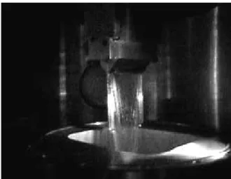
The waterfall target system provides a target for ex-periments on 16_{O. Using a waterfall for oxygen} exper-iments has many advantages. Pure oxygen is difficult to handle, as it is highly reactive. The use of other oxygen compounds requires additional measurements to subtract the non-oxygen background, whereas the hy-drogen in water can be used for calibration purposes. The technique of using continuously flowing water as an electron-scattering target was first developed by Voe-gler and Friedrich [13], and later refined by Garibaldi et al. [12]. The waterfall foil is produced in a cell mounted in the standard scattering chamber. Water forced through slits forms a flat rectangular film which is stable as a result of surface tension and adherence to stainless steel poles (see Fig. 3). The water, continuously pumped from a reservoir, goes through a heat exchanger into the target zone and then back into the reservoir. All parts in con-tact with the water are made of stainless steel. Once the target is formed the thickness increases with the pump speed up to a maximum value that depends on the di-mension of the slits and the stainless steel poles [12]. A factor of ∼ 3 magnification is possible (see Fig. 2).

The target thickness stability is monitored by contin-uously measuring the pump speed, the flow rate and the electron rate. The target is designed to stay at a fixed angular position. Care has to be taken in choosing the window material because of the risk of melting for high beam currents (50 µA in this case). The entrance and

FIG. 3. View of the target cell with the waterfall

exit windows are circular (30 mm in diameter) and made of Be (75 µm thick). Because Be is highly toxic, it has been plated with 13 µm of Ni and a monolayer of Au (which also serves to improve heat conductivity). Under the cell a target frame holds up to five solid targets. A target position can be selected remotely by a mechani-cal system driven by stepping motors and controlled by absolute encoders whose precision is 0.1 mm.

The presence of the hydrogen has many advantages. In particular, it permits a calibration of the missing-mass scale and thus an accurate measurement of the Λ-binding energy in the hypernucleus. The Λ-peak position from the reaction on hydrogen can be obtained using the nom-inal central values for the kinematic variables, and then constrained to be zero by applying a small shift to the energy of the beam (the quantity with the largest uncer-tainty). This shift is common to reactions on hydrogen and oxygen and therefore its uncertainty does not affect the determination of the binding energies of the16

ΛN lev-els.

E. Detector package

The detector packages of the two spectrometers are de-signed to perform various functions that include trigger-ing to activate the data-acquisition electronics, collect-ing trackcollect-ing information (position and direction), precise timing for time of flight measurements and coincidence determination, and identification of the scattered parti-cles. The timing information as well as the main trigger is provided from scintillators. The particle identification is obtained from threshold ˇCherenkov type detectors (aero-gel and gas) and lead-glass shower counters. The main part of the detector package in the two spectrometers (trigger scintillators and vertical drift chambers) is iden-tical. For details, see [9].

1. Tracking

The HRS’s have small acceptance. Tracking informa-tion is provided by a pair of vertical drift chambers in each spectrometer. A simple analysis algorithm is suffi-cient because multiple tracks are rare.

2. Triggering

There are two primary trigger scintillator planes (S1 and S2), separated by a distance of about 2 m. The time resolution per plane is approximately 0.30 ns. For experiments which need a high hadron trigger efficiency, an additional scintillator trigger counter (S0) can be in-stalled. The information from the gas ˇCherenkov counter can be added into the trigger. A coincidence trigger is made from the time overlap of the two spectrometer trig-gers in a logical AND unit. The various trigger signals go to the trigger supervisor module which starts the data-aquisition readout.

3. Particle IDentification (PID)

a. Time Of Flight (TOF) The long path from the target to the HRS focal plane (25 m) allows accurate time-of-flight identification in coincidence experiments if the accidental rate is low. After correcting for differences in trajectory lengths, a TOF resolution of ∼ 0.5 ns (σ) is obtained. The time-of-flight between the S1 and S2 planes is also used to measure the speed of particles, β, with a resolution of 7% (σ).

b. Shower Counters Two layers of shower detec-tors [9] are installed in each HRS. The blocks in both layers in HRS-L and in the first layer in HRS-R are ori-ented perpendicular to the particle tracks. In the second layer of HRS-R, the blocks are parallel to the tracks. Typical pion rejection ratios of 500:1 are achieved using two-dimensional cuts of the energy deposited in the front layer versus the total energy deposited.

c. Gas ˇCherenkov A gas ˇCherenkov detector filled with CO2 at atmospheric pressure [14] is mounted be-tween the trigger scintillator planes S1 and S2. The detector allows an electron identification with 99% ef-ficiency and has a threshold for pions at 4.8 GeV/c. The detector has ten light-weight spherical mirrors [15] with 80 cm focal length, each viewed by a photo-multiplier tube (PMT) (Burle 8854). The focusing of the ˇCherenkov ring onto a small area of the PMT photocathode leads to a high current density near the anode. To prevent a non-linear PMT response even in the case of few photo-electrons requires a progressive high-voltage divider. The length of the particle path in the gas radiator is 130 cm for the gas ˇCherenkov in the HRS-R, leading to an av-erage of about twelve photoelectrons. In the HRS-L, the gas ˇCherenkov detector in its standard configuration has a pathlength of 80 cm, yielding seven photoelectrons on

average. The total amount of material in the particle path is about 1.4% X0. Because of its reduced thickness, the resolution in HRS-L is not as good as that of the shower detector in HRS-R. The combination of the gas ˇ

Cherenkov and shower detectors provides a pion suppres-sion above 2 GeV/c of a factor of 2 × 10−5_{, with a 98%} efficiency for electron selection in the HRS-R.

d. Aerogel Cherenkovˇ There are two aerogel ˇ

Cherenkov counters available with different indices of refraction, which can be installed in either spectrometer and allow a clean separation of pions, kaons, and protons over the full momentum range of the HRS spectrometers. The aerogel is continuously flushed with dry CO2 gas. The two counters (A1 and A2) are diffusion-type aerogel counters. A1 has 24 PMT’s (Burle 8854). The 6 cm thick aerogel radiator used in A1 has a refractive index of 1.015, giving a threshold of 2.84 (0.803) GeV/c for kaons (pions). The average number of photoelectrons for GeV electrons in A1 is ∼ 8. The 9 cm thick aerogel radiator used in A2 has a refractive index of 1.055, giving a threshold of 1.55 (2.94) GeV/c for kaons (protons). It is viewed by 26 PMT’s (Burle 8854). Trigger logic is used to require that A1 not fire (e.g., rejecting pions) but that A2 does fire (requiring kaons). Rejection factors of 70:1 for rejecting pions and > 60:1 for protons were achieved using the aerogels in the hardware trigger.

e. Ring Imaging ˇCherenkov Detector (RICH) In or-der to reduce the background level in produced spec-tra, a very efficient PID system is necessary for unam-biguous kaon identification. In the electron arm, the gas ˇCherenkov counters give pion rejection ratios up to 103_{. The dominant background (knock-on electrons) is} reduced by a further 2 orders of magnitude by the lead glass shower counters, giving a total pion rejection ra-tio of 105_{. The standard PID system in the hadron arm} is composed of two aerogel threshold ˇCherenkov coun-ters [9, 16] (n1 = 1.015, n2 = 1.055). Charged pions (protons) with momenta around 2 GeV/c are above (be-low) the ˇCherenkov light emission threshold. Kaons emit ˇ

Cherenkov light only in the detector with the higher in-dex of refraction. Hence, a combination of the signals from the two counters should distinguish among the three species of hadrons. However, due to possible inefficien-cies and delta-ray production, the identification of kaons could have significant contamination from pions and pro-tons resulting in an unacceptable signal-to-noise ratio in the physics spectra. For these reasons the need for an un-ambiguous identification of kaons has driven the design, construction, and installation of a RICH detector in the hadron HRS focal plane detector package. The layout of the RICH is conceptually identical to the ALICE HMPID design [17]. A detailed description of the layout and the performance of the RICH detector can be found in [18– 20]. It uses a proximity-focusing geometry (no mirrors in-volved), a CsI gaseous photocathode, and a 15 mm thick liquid perfluorohexane radiator [17]. Fig. 4 shows the layout and the working principle of the adopted solution. The ˇCherenkov photons, emitted along a conic surface

FIG. 4. Layout and working principle of the freon CsI prox-imity focusing RICH.

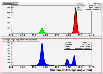
in the radiator, are refracted by the perfluoro-hexane (C6F14)-quartz-methane interface and strike a cathode plane segmented in small pads after traversing a proxim-ity gap of 10 cm filled with pure methane. The photon detector is made of a multi-wire proportional chamber (MWPC), with one cathode formed by the pad planes allowing for the 2-dimensional localization of the photon hit. Three photocathode modules of dimensions 640×400 mm2 _{segmented in 8 × 8.4 mm}2 _{pads are assembled} to-gether for a total length of 1940 mm. The pad planes are covered by a thin (300 nm) substrate of CsI which acts as photon converter. The emitted photoelectron is acceler-ated by an electrostatic field between the pad plane (the cathode of the MWPC) and an anode wire plane at a dis-tance of 2mm from it. The induced charge on the pads is read out by a front-end electronics based on GASSI-PLEX chips. A total number of 11520 pad channels are read out by CAEN VME V550 Flash ADC modules [17]. f. Performance The RICH worked successfully dur-ing the experiment [21] where hadrons were detected in the momentum range p = 1.96 ± 0.1 GeV/c. The average number of photoelectrons detected for pions is Nπ= 13 while for protons Np = 8, their ratio being in perfect agreement with the expected ratio of produced photons at 1.96 GeV/c. In Fig. 5 the reconstructed ˇCherenkov angle distributions are reported. In the top panel the angular distributions have been obtained using samples of π+_{, K}+ _{and p as selected by the two aerogel} coun-ters. The kaon selected sample is practically not visible due to the very high pion to kaon ratio. For the domi-nant contribution of pions the obtained angle resolution is σc= 5 mrad, in agreement with Monte Carlo simula-tions [21]. The kaon contribution is shown in the bot-tom panel where a large sample of aerogel kaon selected events has been used. The reconstructed ˇCherenkov an-gle variable can be clearly used to get rid of the pion and proton contamination. With a resolution σc= 5 mrad the separation between pions and K is about 6σ. The

perfor-FIG. 5. ˇCherenkov angle distributions for protons (thetaC = 0.54 rad), kaons (thetaC = 0.64 rad) and pions (thetaC = 0.68 rad). The aerogel particle selection has been used as explained in the text

.

mance reported here has been obtained with a measured quantum efficiency of about 25% at 160 nm [20]. The RICH pion rejection factor can be estimate to be ∼ 1000 from the pion peak content reduction factor.

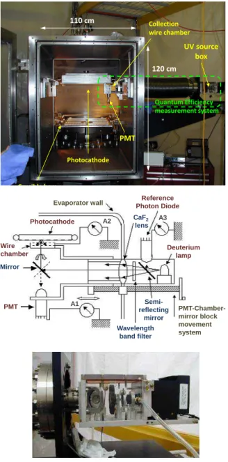
g. The Evaporator A dedicated facility has been built for CsI evaporation of large area photocathodes. It consists of a cylindrical stainless steel vessel (110 cm height, 120 cm in diameter) equipped with four crucibles containing CsI powder (see Fig. 6). A vacuum of a few 10−_{7 mbar can be reached in less than 24 h. The} pre-polished pad plane (a printed circuit with three layers of metals, nickel, copper, and gold, glued on the vetronite substrate) is housed in the vacuum chamber and heated to 60◦ _{C usually for 12−24 h. The location of the} cru-cibles with respect to the photocathode and their relative distance are optimized to ensure a minimum variation in thickness of 10% using equal amount of CsI in each cru-cible. The CsI powder evaporates at a temperature of ∼ 500 C. In order to monitor the quality of the evap-oration and its uniformity, an online quantum-efficiency measuring system has been built and successfully em-ployed [20] (see Fig. 7). A movement system allows us to map out the entire photocathode. A deuterium lamp has been used as UV source light. The UV collimated beam (1 cm in diameter) is split by means of a semi-transparent mirror in such a way to allow monitoring of the lamp emission by measuring the current from a photodiode. Three narrow band filters (25 nm FWHM spread) selecting respectively 160, 185 and 220 nm have been employed. The UV beam is sent, through a ro-tatable mirror, to the photocathode. The photocurrent, generated by electrons extracted from the CsI film, is de-tected with a small (5 × 5 cm2_{) wire chamber located at} a distance of 2 mm from the photocathode. The wires have a collection voltage of 133 V. A second wire plane, behind the first and oriented perpendicular to it, is kept

Crucible bars Photocathode PMT Collection wire chamber 110 cm 120 cm UV source box Quantum Efficiency measurement system A3 A2 A1 Reference Photon Diode Evaporator wall CaF2 lens Deuterium lamp Semi- reflecting mirror PMT-Chamber-mirror block movement system Wavelength band filter Photocathode Wire chamber PMT Mirror

FIG. 6. The CsI evaporator system

FIG. 7. The Quantum Efficiency measurement system.

at ground potential to obtain good charge collection on the first plane. After measuring the wire-chamber pho-tocurrent (A2), the light is sent to a calibrated PMT, used in diode mode (A1), by rotating the mirror. The currents (1250 nA range) are measured by a picoamme-ter (KEITHLEY 485). The ratio of the currents A2/A1, multiplied by the PMT quantum efficiency, gives the “ab-solute” quantum efficiency of the photocathode. Follow-ing the prescription of the ALICE HMPID evaporation system, we have operated our system in such a way to deposit a 300 nm CsI film. This thickness should guaran-tee safe operation of photocathode. In fact no difference in quantum efficiency has been observed in the 150 − 700 nm range [20]. The thickness of 300 nm has been cho-sen as a compromise for having a “stable” photocathode, while avoiding charging up problems at high radiation fluxes. An evaporation speed of 2 nm/s has been chosen as a compromise between the need of avoiding CsI disso-ciation (high crucible temperature, high speed) and the need of avoiding residual gas pollution on the CsI film surface [20].

III. DATA ANALYSIS

A. Missing Energy reconstruction

Event by event, the values of the missing energy were reconstructed by using the detected momenta in the HRS arms and the incident beam energy, assuming the mass of the target nucleus and neglecting its recoil momentum. The missing energy is computed from

Emiss= mK− MA+p(ω + MA− EK)2− (~q − ~pk)2 . (2) The central value and the spread of the beam energy were continuously monitored by OTR or SLI measuments and by the Hall A Tiefenback measurement, re-spectively. Those values were added to the data stream every 30 s.

B. Event Selection

In the selection of the events, significant data reduc-tion is obtained by applying track quality selecreduc-tions and the PID requisites on the threshold ˇCherenkov counters, shower counters, and RICH detector. Only events in which the particle traveling HRS-L was a kaon and the particle traveling HRS-R was an electron were selected.

In addition, selection on the value of the HRS-L/HRS-R coincidence time (2 ns window) were applied to the event in order to be included in the calculation of the missing-energy spectrum. Events corresponding to in-valid values of OTR or SLI were excluded.

FIG. 8. Hadron plus electron arm coincidence time spectra. Left panel: the unfilled histogram is obtained by selecting kaons with only the threshold aerogel ˇCherenkov detectors. The filled histogram (expanded in the right panel) also in-cludes the RICH kaon selection. The remaining contamina-tion is due to accidental (e, e′_{) ⊗ (e, K}+_{) coincidences. The π} and p contamination is clearly reduced to a negligible contri-bution.

C. Particle IDentification (PID)

As pointed out previously the PID capability of the HRS’s, basically guaranteed by TOF, by shower counters in HRS-R and by aerogel counters in the HRS-L, is not sufficient for unambigous kaon identification. A RICH was built for this purpose. The fundamental role of the RICH in identifying the kaons is shown in Fig. 8.

In the left panel, the unfilled timing spectrum of coin-cidences between the electron and the hadron spectrome-ters, obtained by selecting for kaons using the two thresh-old aerogel counters, shows a barely visible kaon signal with a dominant contribution from mis-identified pions and protons. The flat part of this spectrum is given by random coincidences. The 2 ns structure is a reflection of the pulse structure of the electron beam. The filled spec-trum and its exploded version (right panel), is obtained by adding the RICH to the kaon selection. Here, all con-tributions from pions and protons completely vanish.

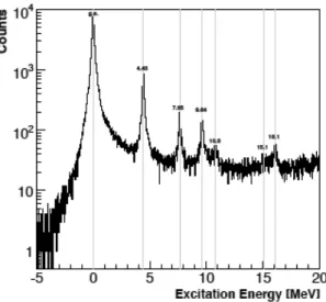
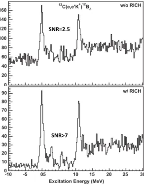
The crucial role of the RICH can be seen also from Fig. 9 that clearly shows that the core-excited states of 12

ΛB are only barely seen if the RICH is not used in the analysis. In that case, the signal to noise ratio is insuffi-cient.

D. RICH

A new particle rejection algorithm based on the χ2 test was employed with the RICH used in the E94-107 experiment to distinguish kaons from pions and protons. It can be essentially summarized in the following steps (more details can be found in reference [22]).

• Identification of the minimum ionizing particle

SNR=2.5

SNR>7

FIG. 9. Excitation energy spectra of12

ΛB with and without the RICH analysis.

(MIP) and ˇCherenkov photon hit points on the RICH cathode. When an MIP crossed the RICH, and it and the ˇCherenkov photons generated in the RICH radiator hit the RICH cathode plane, the pads near their hit points on the cathode gener-ated charge signals. In the following, we refer to the single series of contiguous cathode pads fired by the MIP and the ˇCherenkov photons on the RICH cathode plane as clusters. The cluster corre-sponding to the MIP hit point was easily identified by calculating the interception point between the particle track provided by the drift chambers lo-cated on the focal plane of the HRS spectrometer and the RICH pad plane. The maximum charge cluster inside a defined radius R around this point was assumed to be the one generated by the MIP. All the other clusters on the cathode plane whose distance to the MIP cluster position were compati-ble, within the experimental uncertainties, with the generation of a ˇCherenkov photon in the RICH ra-diator by a proton, kaon or pion whose momentum was equal to the one measured by the HRS spec-trometer were considered as candidate to be gen-erated by a ˇCherenkov photon hitting the cathode plane. A cluster could be made up by one or more pads.

• Cluster resolving. The presence of two or more rela-tive maximums in the geometric distribution in the RICH cathode plane of the pad signals of one single cluster indicated that that cluster was produced by two or more ˇCherenkov photons whose hit points

on the cathode plane were so close that their corre-sponding clusters geometrically overlapped. These clusters were resolved (that is were decomposed into their constituent clusters) by considering that they were generated by a number of ˇCherenkov photons equal to the cluster relative maximum number. The charge assigned to each of the sin-gle clusters constituting an unresolved cluster was proportional to the charge of the corresponding rel-ative maximum.

• Single-photon ˇCerenkov angle determination. The emission angle of each single ˇCherenkov photon generated by the MIP in the RICH radiator was determined from the relative position of the corre-sponding cluster and the MIP cluster in the RICH cathode pad plane and from the direction of the particle track with respect to the normal to the RICH cathode pad plane, using an algorithm based on a geometrical back-tracking.

• Particle identification based on the χ2 _{test. After} the MIP cluster identification and the determina-tion of N ˇCherenkov angles by the back-tracking from the N resolved clusters candidate to be gener-ated by ˇCherenkov photons were performed, three χ2 _{tests were performed, one for each of the three} possible hypotheses (proton, kaon or pion) for the MIP crossing the RICH. In fact, the measured

ˇ

Cherenkov angle distribution around the true value was expected to follow with good approximation a Gaussian distribution. As a consequence the sum P

i

θexpected−θi

σ2 , with θi the ith Cherenkov angleˇ measurement, σ the ˇCherenkov angle measurement distribution, and θexpected the expected ˇCherenkov photon emission angle according to the particle hy-pothesis, is expected to follow the χ2 _distribution if the particle hypothesis is correct and no clus-ter generated by electronic noise was present. The particle was hence identified with the one whose corresponding θexpected value was such that the re-lated χ2 _{test provided a result acceptable within} a predefined confidence level. If none of the three χ2_{tests was acceptable, this meant that electronic} noise was present and one, two, . . . M terms, start-ing with the largest contributor to the χ2_{s, were} iteratively removed until (at least) one of the three χ2_{values, and hence of the particle hypotheses, was} compatible with the significance level.

• Particle identification based on the single-photon ˇ

Cherenkov angle average calculation. Complemen-tary to the particle identification based on the χ2 test was the traditional identification based on the calculation of the average of the N θi measure-ments. This average, when the electronic noise is negligible, is distributed around the true value with a standard deviation equal to σ

sqrtN and hence its comparison with the three expected ˇCherenkov

emission angles corresponding to the three parti-cle hypotheses is a powerful partiparti-cle identification method.

• Particle identification based on the combined use of the χ2 _{test and of the single photon ˇCerenkov} an-gle average calculation. The χ2_{test is a test on the} variance of the N ˇCherenkov angle measurement’s Gaussian distribution. The check on the average of the N ˇCherenkov angle measurements is a test on the mean of this distribution. Mean and vari-ance of a Gaussian distribution are independent pa-rameters. It can be mathematically demonstrated that the χ2 _{test and the test on the average of the} N ˇCherenkov angle measurements are hence two independent tests and can be used simultaneously to obtain proton and pion rejection factors nearly equal to the product of the single test rejection fac-tors, the deviation from an exact product being due to analysis speed considerations and to the presence of electronic noise.

• Use of the aerogel ˇCerenkov detectors for an inde-pendent complete PID. The ˇCherenkov detectors were used in addition to the RICH to obtain a 100% proton and pion rejection with no loss of kaon de-tection efficiency.

The combined use of the two algorithms provided, in combination with the thresholds of two aerogel ˇCerenkov detectors, a completely satisfactory pion rejection ratio greater than 30000 with practically no loss of statistics.

Based on checks against expected values of the average and the variance of the experimental measurements (two statistically independent variables), this algorithm can be employed not only with the RICH’s but whenever one deals with detectors that provide independent multiple measurements of variables with a constant probability distribution function.

E. Normalization

In order to calculate absolute cross sections, the miss-ing energy spectrum has to be properly normalized. The cross section for a level i is computed as

σi= Ni

l surv(k)ǫeǫHǫcoinc∆e∆k∆pe

, (3)

where Niis the number of counts in the level i, corrected for the deadtime, l is the luminosity, surv(k) is the kaon survival probability inside the left arm of HRS, ǫe and ǫk are the detector efficiencies for the two HRS arms, ǫcoinc is the efficiency of the coincidence trigger, ∆eand ∆k are the HRS geometric acceptances for the two arms, and ∆peis the momentum acceptance for electrons.

Since we consider bound states, pk and pe are corre-lated and the cross section is integrated on the full range of ∆pk.

The luminosity is controlled by means of beam-current monitors and rates of single tracks in HRS arms. The dead time is controlled by means of proper data acqui-sition software. Detector efficiencies are controlled by specific analysis software.

F. Beam Current

The measurement of beam current is crucial for cross section determination. For this purpose, the beamline is equipped with two beam-current monitors about 24.5 m upstream of the target. A beam-current monitor is a cylindrical resonant cavity made of stainless steel with a resonant frequency matching the frequency of the elec-tron beam. We used the average value of the two beam-current monitors for our luminosity calculations.

G. Single Rates

Rates of tracks in single HRS arms were continuously monitored in order to cross check the stability of the lu-minosity and the proper operation of the detectors. If a run periods was showing anomalous values of single rates, it was excluded from the cross-section calculation.

H. Efficiency

We calculated the efficiency of the counter detectors based on the Poisson distribution. Then the efficiency for more than one photoelectron detector is ǫ = 1 − e−Np.e._. The efficiency of the RICH detector was determined by the usage of clean track selection on A1 and A2. For the other components of the detector package, the standard procedures established for the HRS were used [9].

The stability of the detector efficiency was continu-ously monitored for each component of the HRS package. In fact, the track rates of the individual detectors were compared to the corresponding luminosity.

I. Peak Search

A χ2_{-based method was used for the detection of the} peaks in the missing-energy spectra. This method ana-lyzes energy intervals in the spectrum and the width of the intervals is variable in a range consistent with the energy resolution of the experiment. The background in the region of interest is very well reproduced by a linear fit. Then for each energy interval showing an excess of counts with respect to the background, the confidence level of those counts was compared to the fluctuation of the corresponding background. If the confidence level was larger than 99% and a local maximum was found, then the corresponding energy region was fitted with a Gaussian or Voigt curve.

J. Energy Resolution

Since the energy resolution is critical for the exper-imental results, the best computation of all the terms involved in the calculation of the missing energy have to be as precise as possible. Therefore:

• The optics database for both the arms of HRS has to provide the best momentum resolution in an ac-ceptance range as large as possible.

• The beam-energy spread was continuously moni-tored using OTR and SLI in order to exclude the events when the energy spread was not good. • The central beam energy was continuously

moni-tored.

• In the case of a rastered beam, a software proce-dure was used to evaluate the real position of the incident electrons, to correspondingly compute the entrance position of the particles in HRS and thus their momentum.

• An iterative method to check the presence of an unphysical dependence of the missing mass on the scattering variables was performed.

K. Radiative corrections

Standard radiative unfolding procedures were per-formed for 12

ΛB [7] and 16

ΛN [8] hypernuclei while, due to the more complicated structure of the spectrum, a different and relatively new technique was used for9

ΛLi. Here we summarize briefly this technique. Details can be found in Ref. [6]. In the case of9

ΛLi we have utilized the property, mathematically demonstrated in Appendix A of Ref. [6], that the subtraction of radiative effects from an experimental spectrum does not depend on the hypothesis/choice of the peak structure used to fit the spectrum itself, providing that the fit is good enough. This property is very useful when the peak structure un-derlying an experimental spectrum is uncertain and sev-eral theoretical (or simply hypothetical) peak structures fit the experimental spectrum well and it is not obvi-ous which of these structures is “the right one”. The 9_{Be(e, e′K}+₎9

ΛLi reaction with the E94-107 experimental apparatus was simulated with the Monte Carlo SIMC. A single excitation-energy peak produced by this simu-lation is shown by the red curve in Fig. 10 (position and amplitude of the peak are arbitrary). The same figure shows, as a blue curve, a single excitation-energy peak produced by Monte Carlo SIMC simulations in the same conditions but with radiative effects “turned off”. Sev-eral peak configurations, with different number, position and heights of peaks like the one reproduced by the red curve of Fig. 10 fit the 9

ΛLi experimental energy spec-trum. Because of the properties of the subtraction of ra-diative effects from spectra quoted above, all of them

pro-Excitation Energy (MeV) 0 2 4 6 8 10 12 0 200 400 600 800 1000 1200 1400 1600 1800 2000 2200

FIG. 10. Color online. From Ref. [6]. One peak of the ex-citation energy spectrum of the hypernucleus 9

ΛLi obtained through the reaction 9_{Be(e, e}′_K+₎9

ΛLi as predicted by the Monte Carlo SIMC when including all effects (red curve) and turning off the radiative effects (blue curve). Arbitrary units. The position of the peak has been made coincident with the ground state.

duced the same radiative-corrected spectrum determined by turning off the radiative corrections in the SIMC simu-lations, that is by substituting the Fig. 10-red-curve-like peaks with peaks like the one reproduced by the blue curve of Fig. 10. Because the Monte Carlo fits to the experimental spectrum were not perfect, slightly differ-ent radiative corrected spectra were obtained from the different peak configurations. The biggest of these differ-ences was assumed as the systematic error generated in the reconstruction of the radiative corrected spectrum by the method employed to generate it. This systematic er-ror was in any case negligible compared to the statistical error.

The unfolding of radiative corrections has been done bin-by-bin. Defining the “Radiative Corrected Monte Carlo” spectrum as the radiative-corrected spectrum ob-tained with the procedure described above and the “Reg-ular Monte Carlo” spectrum as the spectrum produced by the SIMC simulations without turning off radiative corrections that fits the experimental spectrum (this spectrum could be obtained, as quoted above, with dif-ferent peak configurations), the content of each bin of the radiative-corrected spectrum was obtained by multiply-ing the correspondmultiply-ing bin of the experimental spectrum by the correction factor given by the ratio of the Radia-tive Corrected Monte Carlo spectrum and the Regular Monte Carlo spectrum for that bin. In order to avoid possible removals of background enhancements or to arti-ficially zero the spectrum in the regions where the Radia-tive Corrected Monte Carlo spectrum was zero, the ratio between the Radiative Corrected Monte Carlo spectrum and the Regular Monte Carlo spectrum was performed after summing the background for each of them. The

background value was then subtracted from the result of the product of the ratio with the corresponding bin.

Once the radiative corrections were applied, the binding-energy spectrum resolution is small enough to clearly show the three-peak structure shown in Fig. 15.

L. Calibrations 1. Optics

The quality and exact character of the optics trans-formation tensor were measured with a series of elastic scattering measurements using a 2 GeV electron beam on C and Ta targets. Measurements were also made using a sieve-like mask in front of each spectrometer to optimize and calibrate the angular reconstruction. Finally, a check on residual correlations between the missing energy and the optics variables was performed by a dedicated itera-tive method. This method [23] was based on the prop-erty that any change in the optical data base corresponds mathematically to an addition, to the missing-mass nu-meric value, of a polynomial in the scattering coordi-nates of the secondary electron and of the produced kaon. The method consisted of checking whether the numerical missing-mass value produced by the optical data base had unphysical mathematical dependencies on the electron and kaon scattering variables. Fitting these mathemati-cal dependencies with a polynomial P , the method con-sisted in finding the change in the optical data base that produced an addition to the calculated numerical value of the missing mass equal to −P and that hence eliminated the unphysical missing-mass dependency. Once any pos-sible dependency of the numerical value of the missing mass on the scattering coordinates had been eliminated with the method described above, the optic data base was optimized. In fact, any further change in the optic data base would have meant the addition of a polyno-mial in the scattering coordinates to the numerical value of the missing mass that would have produced new un-physical dependencies. The method described above is based on physics considerations. It also usually produces the best resolution. In fact, unphysical dependencies of the missing-mass numerical value on the scattering coor-dinates means that the missing-mass values as produced by the optic data base spread around the true binding-energy values as function of the scattering coordinates increasing the FWHM of the missing-energy spectrum peaks.

The results of the calibration and optimization effort are illustrated in Fig 11.

2. Waterfall target

A calibration of the target thickness as a function of pump speed has been performed.The thickness was de-termined from the elastic cross section on hydrogen [12].

FIG. 11. Elastic 12_{C scattering spectrum as seen in one arm} of the HRS + Septum configuration after optimization. The width of all the peaks, elastic and inelastic, is 10−4_(FWHM

The target thickness used was 75 ± 3 (stat.) ± 12 (syst.) mg/cm2_.

3. Energy scale

Careful calibration methods were employed to deter-mine the binding-energy spectra of the hypernuclei 16

ΛN and9

ΛLi, and of the excitation-energy spectrum of the hy-pernucleus 12

ΛB. These methods were necessary because the actual kinematics of the processes producing the hy-pernuclei quoted above differed from the nominal ones by amounts that would have produced significant shifts and distortions in binding-energy and excitation-energy spectra if proper measures had not been taken. In fact, while the actual kinematics values in the experiment, pro-vided by the CEBAF accelerator electron beam energy and by the central momenta and angles of the HRS elec-tron and hadron arms, could be considered constant for the entire course of the experiments (their variations be-ing of the order of 105_{for the CEBAF electron-beam} en-ergy and the central momenta of the HRS electron and hadron arms, and practically zero for the spectrometer central angles), they differed by unknown amounts, re-ferred to as “kinematical uncertainties” in the following, from their nominal values, that is the values the CE-BAF beam energy and the HRS central momenta and angles were nominally set at according to the kinemat-ics of the experiment. Although small (the experimental uncertainties on the CEBAF accelerator electron-beam energy and on the spectrometer central momenta being of the order of 104 _{to 10}3 _{and those on the} spectrome-ter central angles of the order of 102_{), these} kinemati-cal uncertainties have two non-negligible effects a) they

Excitation Energy (MeV)

-100 -80 -60 -40 -20 0 20 40 60 80 100

Counts (150 keV bin)

0 10 20 30 40 50 60 Σ , Λ ), + p(e,e’K

FIG. 12. Excitation energy spectrum of the p(e, e′_K+_{)Λ, Σ}0 on hydrogen used for energy scale calibration. The fitted po-sitions (not shown on the plot) for the peaks are −0.04 ± 0.08 MeV and 76.33 ± 0.24 MeV.

cause global shifts in the binding-energy spectra and b) they cause peak distortions increasing their FWHM in the binding/excitation-energy spectra. The actual kine-matics values in an experiment are then those that po-sition states at their known value in binding/excitation energy spectra and minimize peak FWHM’s.

To calibrate the binding-energy scale for 16

ΛN, the Λ peak position from the reaction on hydrogen was first obtained using the nominal central values for the kine-matic variables, and then constrained to be zero by ap-plying a small shift to the energy of the beam (the quan-tity with the largest uncertainty). This shift is com-mon to reactions on hydrogen and oxygen and there-fore its uncertainty does not affect the determination of the binding energies of the 16

ΛN levels. A resolution of 800 keV FWHM for the Λ peak on hydrogen is ob-tained. The linearity of the scale has been verified from the Σ0_{−Λ mass difference of 76.9 MeV. For this purpose,} a few hours of calibration data were taken with a slightly lower kaon momentum (at fixed angles) to have the Λ and Σ0 _{peaks within the detector acceptance. Fig. 12} shows the two peaks associated with p(e, e′_K+_{)Λ and} p(e, e′_K+_)Σ0 _{production. The linearity is verified to} (76.9 − 76.4 ± 0.3)/76.4 = 0.65 ± 0.40%

The hypernuclei 12 ΛB and

9

ΛLi were produced in one run where waterfall or hydrogen targets were not avail-able. For these two hypernuclei, the energy-scale cali-bration was hence performed by positioning, in the 12

ΛB binding-energy spectrum, the ground-state peak at its known value of −11.37 MeV determined by emulsion data, after taking into account the additional shift in the energy scale (calculated through Monte Carlo sim-ulations), caused by the energy losses in the target12_C by the participants to the reaction producing the hyper-nucleus12

ΛB. The kinematical uncertainties were further reduced by minimizing the width of 12

peak. This peak is actually a doublet with its two com-ponents separated by ∼ 160 keV. However, this value is small enough with respect to the energy resolution of the experiment to make the approximation of assuming the 12

ΛB ground state as a single peak still valid and make consequently small the distortions incidental to the min-imization of the FWHM of a peak that is actually a dou-blet. No attempt to minimize the FWHM was performed on the other peaks of the12

ΛB spectrum. Because the hy-pernuclei12

ΛB and9ΛLi were produced with the same ap-paratus and the same nominal kinematic variables, the 12

ΛB excitation-energy calibration results where applied to obtain the9

ΛLi binding-energy spectrum, after taking into account the difference between the global shifts of the peaks in the two spectra due to the difference of the particle-energy loss in the12_{C and in the}9_{Be targets.}

M. Systematic errors

The main sources of systematic errors in the missing-energy spectrum are:

• The uncertainty on the value of the beam energy. • The uncertainty on the values of the track

mo-menta.

• The uncertainty on correction for radiative effects. If not specified, our systematic errors on the position of the peaks in the missing-energy spectrum are negligible with respect to their corresponding statistical errors.

For the calculation of the binding energies, an addi-tional contribution to the systematic error has to be con-sidered, due to the need for an absolute energy scale. In the case of12

ΛB the binding energies were not calculated. In the case of16

ΛN this contribution is determined by the uncertainty in the position of the Λ peak obtained from the strangeness production on hydrogen in the waterfall target. In the case of 9

ΛLi, an additional contribution to the systematic error is due to the uncertainty of the knowledge of the12

ΛB ground-state binding energy, which we used as reference.

For the calculation of absolute cross sections, the fol-lowing sources of systematic uncertainties were consid-ered:

• The uncertainty on the integrated beam current. • The uncertainty on the target thickness. It is 2%

for solid targets. For the oxygen in the waterfall target it is 16% as previously quoted.

• The uncertainty on the detector efficiencies. • The uncertainty on the dead-time correction • The uncertainty on the HRS phase space.

• The uncertainty on the corrections for radiative ef-fects.

Based on the run-by-run fluctuations, we evaluated our global systematic error on absolute cross sections as being within 15% for 12

ΛB and within 20% for 16ΛN and 9ΛLi. Due to the different contributions of the radiative effects, systematic errors were individually calculated for each peak in the missing-energy spectra.

IV. THEORY

A. Electroproduction of hypernuclei in DWIA Production of hypernuclei by a virtual photon associ-ated with a kaon in the final state can be satisfactorily de-scribed in the distorted-wave impulse approximation [24] because the photon and kaon momenta are rather high (≈ 1 GeV). The cross section for the production of the ground or excited states of a hypernucleus depends on the many-particle matrix element between the nonrela-tivistic wave functions of the target nucleus (ΨA) and the final hypernucleus (ΨH) T_ifµ = hΨH| Z X j=1 χγχ∗KJ µ j|ΨAi. (4)

Here J_jµ is the hadronic current corresponding to elec-troproduction of a Λ on the proton (the elementary pro-duction). The sum runs over the protons of the target nucleus as we study K+ _{electroproduction. In the} one-photon approximation, the virtual one-photon is described by the function χγ proportional to the product of the wave functions of incoming and outgoing electrons with-out Coulomb distortion. The kaon distorted wave χK is calculated in the eikonal approximation from a first-order optical potential in which the density of the hypernu-cleus is approximated by that of the target nuhypernu-cleus. The eikonal approximation is sufficient for weakly interacting kaons with momenta larger than 1 GeV.

The kaon-nucleus optical potential is constructed using the kaon-nucleon total cross section and the ratio of the real to imaginary parts of the forward scattering KN am-plitude. The amplitude is properly isospin averaged to take into account the number of protons and neutrons in the nucleus. The KN amplitudes for isospin 0 and 1 are calculated in a separable model [25] with partial waves l = 0, 1, ...7 and with parameters recently fitted to the phase shifts and inelasticity parameters in the KN scat-tering. The nuclear density in the potential is modeled by the harmonic-oscillator form with the constant taken from experiments on the nucleus charge radii.

The matrix element is calculated in the frozen-nucleon approximation (the target proton three momentum in the laboratory frame is zero) which significantly simplifies the integration and allows one to express the elementary plitude in the laboratory frame via only six CGLN am-plitudes [24]. To go beyond this factorization approach, i.e. include also a Fermi motion in the nucleus, one would have to calculate the elementary amplitude in a general

reference frame which would, together with the momen-tum integration, make the calculation considerably more complicated.

Experiments on electroproduction of hypernuclei are performed in the kinematical region of almost real pho-tons (Q2_{= −q}2

γ ≈ 0). In this kinematics, the elementary electroproduction cross section is dominated by its trans-verse part and can be approximated by the photoproduc-tion cross secphotoproduc-tion - e.g., as in Ref. [26]. However, even at values of Q2_{as small as those in Table I, the} transverse-longitudinal interference contribution can be important. That is why in the calculations presented here, the full electroproduction cross section is used [24].

B. Elementary production process

The hadronic current, expressed in the non-relativistic two-component formalism via six CGLN amplitudes in the laboratory frame, is calculated using an isobar model [24, 27]. Due to the strong damping of the hypernuclear production cross section by the nucleus-hypernucleus form factors for large kaon angles, the dom-inant contribution from the elementary amplitudes comes from the region of very small kaon angles. In this kine-matical region, however, the various isobar models give big differences in predicted cross sections, especially for Elab

γ > 1.7 GeV [26, 28, 29], see also Sect. V A. The mag-nitude of these differences constitutes an important part of the theoretical uncertainty in predicting the hypernu-clear production rate. For the energies of the Hall A ex-periments, Elab

γ = 2.2 GeV, the Saclay-Lyon model [30] gives very good results for the hypernuclear cross sec-tions [6–8]. In our analysis, we also use a very recent isobar model BS3 [31] that fits the new data on photo-and electroproduction well photo-and also gives reasonable pre-dictions for the cross sections at small kaon angles. Note that the JLab data on the Q2 _{dependence of the} sepa-rated transverse and longitudinal cross sections are sig-nificantly better described by the BS3 model than by the Saclay-Lyon (SLA) model as is shown in Fig. 13 of Ref. [31]. It is, however, fair to say that, in contrast to BS3, the SLA model was not fitted to these data.

C. Nucleus and hypernucleus wave functions The wave functions for light hypernuclei are obtained from shell-model calculations using an effective p-shell interaction to describe the nuclear core states [32]. In this weak-coupling approach, both Λ and Σ hyperons in s-states are coupled to p-shell core wave functions opti-mized to fit a wide range of p-shell properties. The ΛN effective interaction can be written in the form

VΛN(r) = V0(r) + Vσ(r)sΛ· sN + VΛ(r)lΛN · sΛ+ VN(r)lΛN · sN + VT(r) S12, (5)

where V0 is the spin-averaged central interaction, Vσ is the spin-dependent central term, VΛand VN are the spin-orbit interactions and VT is the tensor ΛN interaction with S12= 3(σΛ·r/r)(σN·r/r)−σΛ·σN. The quadratic spin-orbit term, also allowed by symmetries, is neglected. For a p-shell nucleon and a Λ in the s orbit the radial integrals can be parameterized via five constants, ¯V , ∆, SΛ, SN, and T

VΛN = ¯V + ∆ sΛ· sN + SΛlΛN · sΛ+

SN lΛN · sN + T S12, (6)

which have a one-to-one correspondence with the five pNsΛ two-body matrix elements. The last four matrix elements can be determined from the analysis [32] of pre-cise γ-ray spectra of p-shell hypernuclei obtained via hy-pernuclear γ-ray spectroscopy, mostly with the Hyper-ball [4]. The ΣN and ΛN -ΣN coupling matrix elements can be parametrized in the same way with the values of the parameters calculated using Woods-Saxon wave functions and Gaussian or Yukawa representations of Y N G-matrix elements based on free Y N baryon-baryon po-tentials [33]. The Λ-Σ coupling makes significant contri-butions to hypernuclear doublet spacings but, while in-cluded in the shell-model calculations, is not important for analyses of (e, e′_K+_{) data.}

Unfortunately, γ-ray spectroscopy is feasible only for hypernuclear states lying below particle thresholds. Information about the structure of multiplets above particle-emission thresholds, generally when the Λ is in a p orbit, is provided by analyses of the missing-mass spec-tra from electroproduction (reaction spectroscopy) which can be realized with better energy resolution than from the pion or K− _{induced production reactions [4].}

After the partial-wave decomposition of the wave func-tions χγχ∗K, the many-body matrix element (4) can be expressed by means of the hypernucleus-nucleus struc-ture constants, radial integrals, and the CGLN ampli-tudes. The structure constants are calculated from one-body density matrix elements provided by the shell-model structure calculations with the interaction (5). In the radial inegrals, we make use of the Woods-Saxon single-particle wave functions for the target proton and final Λ which we suppose to be a more realistic approx-imation than the harmonic oscillator wave functions, es-pecially in the case of weakly bound particles. The pa-rameters, the radius, slope, and potential depth of the Woods-Saxon potential, which includes the central, spin-orbital, and Coulomb parts, are taken from other pro-cesses. The single-particle binding energies correspond to the particle separation energies.

The two-body matrix elements for hyperons in 0p or-bits (20 matrix elements for pNpΛ) for use in the shell-model calculations (with Λ-Σ coupling included) are like-wise calculated using Woods-Saxon wave functions.