Automatic orthographic alignment of speech

Automatic Orthographic

Alignment of Speech

by

Jerome S. Khohayting

S.B. Mathematics, Massachusetts Institute of Technology, 1993

Submitted to

the Department of Electrical Engineering and Computer Science in Partial Fulfillment of the Requirements for the Degrees of

Master of Engineering and Bachelor of Science

at the

Massachusetts Institute of Technology

(Jerome Khohayting, 1994 All rights reserved.

The author hereby grants to MIT permission to reproduce and to distribute copies of this thesis document

in whole or in part.

Signature of Author ...epartment

Department

Certified by ...

Dwartment

*---sg -..-... . . . .. . .... ...

of Eldcti al Engineering anComputer Science -~ _, May 12, 1994

. ·Q= H V.,; ; .'. .. , ...

James R. Glass Research Scientist of fectctl Engineer a]id Computer Science

hesis Supervisor Z.N

Accepted

by ... ..

...

Frederic R. Morgenthaler Chairman, Department ommittee on Graduate Students

WITHDRAWNI MASSA INSTITUTE

Automatic Orthographic

Alignment of Speech

by

Jerome S. Khohayting

Submitted to the Department of Electrical Engineering and Computer Science in May, 1994 in partial fulfillment of the requirements for the Degree of

Master of Engineering and Bachelor of Science.

Abstract

The objective of the research is to develop a procedure for automatically aligning an orthographic transcription with the speech waveform. The alignment process was performed at the phonetic level. The words were converted into a sequence of phonemes using an on-line dictionary and a network of phones was created using phonological rules.

The phonetic alignment was accomplished using a microsegment-based approach which utilized a probabilistic framework. Acoustic boundaries were proposed at points of maximal spectral change, and were aligned with the phone network using a time-warping algorithm incorporating both acoustic and durational weights to the score. This approach was then compared to the traditional frame-based technique, which can be interpreted as proposing boundaries at every frame before the process of aligning with the network.

The acoustic as well as the durational models were trained on the TIMIT corpus, and the algorithm was tested on a different subset of the corpus. To investigate the robustness of the procedure, the resulting algorithm was trained and evaluated on the same subsets, respectively, of the NTIMIT corpus, which is the telephone version of the TIMIT utterances. A word overlap ratio of 93.2 % and a word absolute error of 20.4 ms were achieved on the TIMIT corpus. This corresponds to a phone overlap ratio of 81.7 % and a phone absolute error of 12.9 ms.

Thesis Supervisor: James R. Glass Title: Research Scientist

Acknowledgments

I wish to express my deepest gratitude to my thesis advisor, Jim Glass, for all the knowledge, support, patience and understanding he has given me for the last two years. He has devoted a significant amount of his precious time to guide me through my work, and I have learned so much from such occasions. Specifically, I thank him for his help on programming and spectrogram reading.

I also wish to thank all the members of the Spoken Language Systems Group for their friendship. In particular, I would like to thank:

Victor Zue, for letting me join the group, for providing an environment conducive to learning, and for his sense of humor,

Lee Hetherington and Dave Goddeau, for answering a lot of my questions on UNIX, C and LATEX,

Mike Phillips, for creating a lot of the tools I have used, Mike McCandless, for all his help on C and MATLAB, Nancy Daly, for all her help on phonetics,

Bill Goldenthal, for all his interesting insights on interview techniques, sports and machine allocation,

Eric Brill, for all his views on the stock market,

Jane Chang, for being a great officemate and for putting up with me, Christine Pao and Joe Polifroni, for keeping our systems running,

Vicky Palay and Sally Lee, for everything they've done to maintain and organize the group.

Special thanks goes to Tony Eng for reading a draft of my thesis and providing helpful comments. I also thank Mike Ong Hai, Bobby Desai and Daniel Coore for all the good times.

Finally, I wish to thank my parents for all their love and encouragement.

This research was supported by ARPA under Contract N00014-89-J-1332 monitored through the Office of Naval Research, and in part by a research contract from the Linguistic Data Consortium.

Contents

2 Modelling and Classification

2.1 Probabilistic Framework. 2.2 Modelling ... 2.2.1 Phone Classes . . . . 2.2.2 Signal Representation . 2.2.3 Acoustic Modelling ... 2.2.4 Durational Modelling . 2.3 Training ... 2.3.1 Acoustic Models. 2.3.2 Durational Models. 2.4 Classification ... 2.4.1 Frame Classification. 2.4.2 Microsegment Classification . 2.4.3 Segment Classification .... 2.5 Summary ... 3 Boundary Generation 3.1 Independence of Microsegments . . . 3.2 Criteria ... 3.2.1 Deletion Rate . . . . 3.2.2 Boundary-to-Phoneme Ratio .

3.2.3 Errors of Boundary Accuracy

3.3 Parameters ...

3.3.1 Spectral Change and Spectral Derivative ...

9 9 11 12 13 14 15 17 18 ... ...18 . . . 20 . . . 20 . . . 21 . . . 22 . . . 22 . . . 23 . . . 23 . . . 24 . . . 25 . . . 25 . ... .. ... .. . .26 . . . 29 31 32 32 33 33 34 34 35 35

...

...

...

...

...

...

...

...

...

...

...

3.3.2

3.3.3 3.3.4

Peaks in Spectral Change Threshold on the Spectral Threshold on Second Deri 3.3.5 Associations on Acoustic 3.3.6 Constant Boundaries per

3.4 Results . ...

3.4.1 Uniform Boundaries 3.4.2 Acoustic Boundaries 3.4.3 Adding More Boundaries 3.5 Selection. ... 4 Network Creation 4.1 Phonological Variations . 4.2 Rules . ... 4.2.1 Gemination ... 4.2.2 Palatalization ... 4.2.3 Flapping . . . . 4.2.4 Syllabic Consonants 4.2.5 Homorganic Nasal Stop. 4.2.6 Fronting ...

4.2.7 Voicing . . . .

4.2.8 Epenthetic Silence and GI 4.2.9 Aspiration ...

4.2.10 Stop Closures . . . .

5 Alignment Procedure and Evalual

5.1 Search . . . .

5.1.1 Observation-based Search 5.1.2 Full Segment Search 5.2 Alignment ...

5.2.1 Evaluation Criteria . . .

5.2.2 Two-Pass Evaluation 5.3 Full-Segment Search Evaluation 5.4 Summary ...

6 Conclusions

6.1 Summary . . . .

6.2 Comparison To Other Work . . 6.3 Future Work .

...

38

Change ... 38

vative of Spectral Change ... 38

Parameters ... 39 Spectral Change ... 39 . . . 40 . . . 40 . . . 41 . . . 42 . . . 46 48 . . . .48 . . . 50 . . . 50 . . . 50 . . . .52 . . . .53 . . . .53 . . . .53 . . . 53 . . . 54 . . . 55 . . . 55 . . . .. . . . .. . . t . . . . . . . . . Stops . . . . . . 57 . . . ..57 . . . 58 . . . ..60 . . . ..60 . . . 61 . . . 61 . . . ..69 . . . 70 71 71 72 73 A Phone Classes B Phonological Rules 74 76 . . . .- I I

C Alignment Algorithms 79

C.1 Two-Pass Observation-Based Method ... 79 C.2 Full Segment Search Method ... .... 82

D Train and Test Speakers 84

D.1 Train Speakers ... . 84 D.2 Test Speakers ... 85

List of Figures

1.1 Automatic Orthographic Alignment of Speech . . . .... 10

1.2 Schematic Diagram for the Alignment System ... 16

3.1 Time Plots of Acoustic Parameters. ... 37

3.2 Example of Boundary Generation Technique ... 47

4.1 Network Generation ... 49

4.2 Examples of Palatalization . . . ... 51

4.3 Example of Flapping ... 52

4.4 A Contrast of a Fronted and a Non-Fronted [u]. ... 54

5.1 Schematic Diagram for the Observation-Based Method ... 59

List of Tables

2.1 Microsegment Classification Results Using Different Deltas ... 2.2 Microsegment Classification Results Using Different Deltas and

Addi-tional Microsegments ...

2.3 Microsegment Classification Results Using Different Deltas and Three Averages .

2.4 Segment Classification With Automatically Aligned Boundaries . . . 2.5 Exact Segment Classification ...

3.1 Results of Uniform Boundaries ...

3.2 Varying Threshold on Second Derivative of Spectral Change ... 3.3 Results of Associations on Cepstral Coefficients ...

3.4 Results of Associations on Spectral Coefficients ...

3.5 Results of Adding Uniform Boundaries To Second Derivative Threshold 3.6 Adding Constant Boundaries Per Spectral Change To Spectral Change

Threshold.

3.7 Adding Constant Boundaries Per Spectral Change To Second Deriva-tive Threshold ...

3.8 Adding Minimum Distance Criterion to Spectral Change Threshold of 175.0 and Constant Boundaries ...

3.9 Adding Minimum Distance Criterion to Second Derivative Threshold of 10.0 and Constant Boundaries ...

5.1 5.2 5.3 5.4 5.5 5.6 5.7 5.8

Frame Alignment Phone-Level Ideal and First Pass Results Frame Alignment Phone-Level Second Pass Results .... Frame Alignment Word-Level First Pass Results ... Frame Alignment Word-Level Second Pass Results ... Microsegment Alignment Phone-Level Results ... Microsegment Alignment Word-Level Results ...

Full-Segment Search Phone-Level Ideal and Overall Results Full-Segment Search Word-Level Overall Results ... 6.1 Full-Segment Search Word-Level Overall Results ... A.1 Forty-Two Phone Classes in IPA form...

A.2 Forty-Two Phone Classes in ARPABET form ...

26 28 28 30 30 40 41 42 42 43 44 45 46 46

... .

.63

... .

64

... .

64

... .

65

... .

.67

... .

68

... .

70

... .

70

Chapter 1

Introduction

1.1 Overview

Automatic speech recognition has been a tantalizing research topic for many years. To be successful, speech recognizers must be able to cope with many kinds of variability: contextual variability in the realization of phonemes (i.e., coarticulation), variability due to vocal tract differences between speakers and speaking styles, and acoustic variability due to changes in microphone or recording environment. In order to be able to model such variability, researchers use large corpora of speech to train and test acoustic-phonetic models. Corpora are especially useful when orthographically and phonetically aligned transcriptions are available along with the speech [13]. Such corpora are also valuable sources of data for basic speech research. An example of an aligned speech utterance is shown in Figure 1.1. In the figure, the spectrogram for the sentence "Two plus seven is less than ten" is shown, as well as its aligned phonetic and orthographic transcriptions.

Manual transcription of large corpora, however, is extremely time consuming, so automatic methods are desired. There are different degrees of automating this pro-cess. One method would require a phonetic transcription of an utterance before

align-kHz

Time (seeonds)

1 lcoiinpt _ __ I _

t u p p I A S V z ISE n __ t t t _ n #

T wo plus stbrpen lransct then

TWO P/Us seven IJ le than ten. I

Figure 1.1: Automatic Orthographic Alignment of Speech

Digital spectrogram of the utterance "Two plus seven is less than ten" spoken by a male speaker. A time-aligned phonetic and orthographic transcription of the utterance are shown

ing it with the speech signal [14]. A fully automated system would require only the orthography of the utterance, and could generate a phonetic network automatically before aligning it with the waveform. This research focuses on the latter approach.

In the past, researchers have typically used a frame-based approach for phonetic alignment. This research investigates a segment-based approach utilizing a stochastic framework. An on-line dictionary is used to expand words into a baseform phoneme sequence. This sequence is then converted to a phone network by applying a set of phonological rules. The rules are intended to account for contextual variations in the realization of phonemes. The phone sequence which best aligns with the speech signal is determined using the phonetic alignment algorithm.

The aligment procedure is evaluated primarily on the TIMIT [13] and NTIMIT [11] acoustic-phonetic corpus. Comparisons to results reported in the literature are made whenever possible.

1.2 Previous Work

There has been considerable work done on the problem of orthographic transcrip-tion by speech researchers in the past. The method of orthographic transcriptranscrip-tion is normally accomplished by converting the text into possible phone sequences and per-forming phonetic alignments with the speech signal. In this section, the work done on phonetic alignment, as well as the techniques developed for orthographic alignment, are described.

1.2.1 Phonetic Alignment

Frame-based Techniques

The most common approach to phonetic alignment is the use of frame-based proba-bilistic methods. These methods use acoustic models to perform time-alignment based on the frame by frame statistics of the utterance. Dalsgaard [7] used a self-organizing neural network to transform cepstral coefficients into a set of features, which are then aligned using a Viterbi algorithm. Ljolje and Riley [15] used three types of indepen-dent models to perform the alignment algorithm-trigram phonotactics models which only depended on the phoneme sequence on the sentence, acoustic models which used three full covariance gaussian probability density functions, and phone duration models. The three types of models were interrelated through a structure similar to a second order ergodic continuous variable duration HMM (CVDHMM). They re-ported an 80% accuracy for placing the boundaries within 17 milliseconds (ms) of the manually placed ones. In a follow-up work [16], they utilized a similar CVDHMM

structure but performed training and testing on separate utterances spoken by the

same speaker. The results were naturally better-an 80% accuracy within a tolerance

of 11.5 ms was achieved instead. Brugnara [4] and Angelini [2] also used HMM's to model the acoustic characteristics of the frames and the Viterbi algorithm to perform segmentation. Blomberg and Carlson [3] used gaussian statistical modelling for the parametric as well as spectral distributions, and for the phone and subphone dura-tions. Fujiwara [9] incorporated spectrogram reading knowledge in his HMM's and performed the segmentation algorithm.

Segment-based Techniques

An alternative approach was taken by Andersson and Brown [1] and by Farhat [8]. Both initially divided the speech waveform into short segments composed of several

frames having similar acoustic properties. Anderson and Brown classified the sig-nal into voiced/unvoiced segments using a pitch-detection algorithm. Corresponding segments of voiced/unvoiced events were generated from the text, and a warping al-gorithm was used to match the segments. The speech signals used were typically several minutes long and reasonable results were achieved. Farhat and his colleagues compared performing time-alignment using a segmental model to a centisecond one. In the latter approach, mel-frequency cepstral coefficients (MFCC's) were computed every 10 ms and the Viterbi algorithm was used to do the matching. In the former, the speech signal was first segmented with a temporal method. A similar vector of MFCC's was computed every segment, and a similar Viterbi search was employed to perform the alignment. The segmental approach achieved better results; using context independent models, it produced a 25% disagreement with manual labelling allowing a tolerance of 20 ms, as opposed to 35% for the centisecond approach. These works suggest that the segmental methods are at least as successful as their frame-based

counterparts.

Other Techniques

The work of Leung [14] consists of three modules. The signal is first segmented into broad classes. Then these broad classes are aligned with the phonetic transcription. A more detailed segmentation and refinement of the boundaries is then executed. On a test set of 100 speakers, the boundaries proposed by the alignment algorithm were within 10 ms of the correct ones 75% of the time.

1.2.2 Orthographic Alignment

On the more general problem of orthographic transcription, Ljolje and Riley [15] used a classification tree based prediction of the most likely phone realizations as input

for the phone recognizer. The most likely phone sequence was then treated as the true phone sequence and its segment boundaries were compared with the reference boundaries. Wheatley et al [18] automatically generated a finite-state grammar from the orthographic transcription uniquely characterizing the observed word sequence. The pronunciations were obtained from a 240,000-entry on-line dictionary. A separate path through the word-level grammar was generated for each alternate pronunciation represented in the dictionary. The word pronunciations were realized in terms of a set of context-independent phone models, which were continuous-density HMM's. With these phone models, the path with the best score was chosen and an orthographic transcription was obtained.

1.3 Corpus Description

The TIMIT and NTIMIT acoustic-phonetic corpora are used in this thesis. The TIMIT corpus was recorded with a closed-talking, noise-cancelling sennheiser micro-phone, producing relatively good quality speech [13]. It is a set of 6,300 utterances spoken by 630 native American speakers of 8 dialects, each speaking a total of ten sentences, two of which are the same across the training set. The NTIMIT corpus is formed by passing the TIMIT utterances over the telephone line, producing speech which is noisier with a more limited bandwidth [13]. Evaluating alignment algo-rithms on NTIMIT gives an indication of the robustness of the algorithm to different microphones or acoustic environments.

In the training of the TIMIT sentences, a set of 4536 sentences uttered by 567 speakers each speaking eight sentences is used. The training speakers are listed in Ap-pendix D.1. In the evaluation of the TIMIT utterances, a set of 250 sentences uttered by 50 speakers each speaking five sentences is used. The test speakers are listed in Appendix D.2. No test speaker was part of the training set. For the NTIMIT corpus,

the corresponding subsets of the database are used, respectively, for the training and testing procedures.

These corpora come with their phonetic and orthographic sequences, together with the time boundaries for each of these sequences, i.e. the phonetic and orthographic transcriptions. This creates the possibility of a supervised training of the acoustic and durational models used. Moreover, this aids in the testing of the algorithm, because the supposedly correct answer is known and hence can be compared to the transcription derived from the alignment algorithm.

1.4 Transcription Components

The ultimate objective of this thesis is to present a segmental approach to the prob-lem of aligning in time the speech waveform with its orthographic transcription. A schematic diagram for the alignment algorithm is shown in Figure 1.2.

First, acoustic models for each of forty-two phone classes are trained, using mel-frequency cepstral coefficients, described in Section 2.2.2, as the acoustic parameters. Durational models are likewise created.

The second step is to propose phone boundaries from the acoustic data. The idea is that the more boundaries proposed, the chances of the exact boundaries each being located near a proposed boundary is higher. Then it remains to identify these "closest" boundaries among all the ones proposed. Proposing too many boundaries makes this latter problem harder.

The next step is to create a network of possible phone sequence given the ortho-graphic transcription. An on-line dictionary is used to create a baseform phoneme sequence. The phonemes of the words are concatenated together to form the phoneme sequence of the sentence. Then, by applying a set of phonological rules, a network

Acoustic Models

Durational Models

Figure 1.2: Schematic Diagram for the Alignment System

of possible phone sequences is formed from this phoneme sequence. The rules are intended to account for contextual variations in the realization of phonemes.

Then, a Viterbi algorithm is used to traverse through the paths in the network of phone sequences. For each path, a phonetic alignment is performed and a probability is determined. Such a score includes acoustic as well as durational components. The path with the best likelihood is then chosen and consequently an orthographically aligned transcription is achieved.

A frame-based technique in which each frame is proposed as a boundary is also developed. The network creation and alignment procedure is the same as the segment-based approach, and the results are compared. Finally, this whole alignment proce-dure is trained and tested on the TIMIT and the NTIMIT databases.

1.5 Thesis Outline

A brief outline of the thesis is presented here. In Chapter 2, the probabilistic frame-work is presented, and the development and training of acoustic and durational mod-els are described. Classification experiments at the frame, microsegment and phone levels are also carried out.

The boundary generation algorithm is discussed in Chapter 3. The various criteria and parameters are enumerated, and the results are discussed. A set of optimal boundary parameters is selected in the last section.

In Chapter 4, a discussion of the phonological variations is presented, and the various phonological rules used for the network creation are described.

The alignment procedure is described at length in Chapter 5. Two different search methods, the two-pass method and the full segment method, are presented and eval-uated. The two-pass method is observation-based and experiments using frames and microsegments as observations are separately performed.

Finally, a summary of the results of the alignment procedure is presented in Chap-ter 6. Some possible future directions for the problem of time-alignment are also described here.

Chapter 2

Modelling and Classification

The acoustic modelling for the alignment process is presented in this chapter. This includes a discussion of the probabilistic framework as well as the different acous-tic parameters. To test the accuracy of the models, classification experiments are performed, and the results are analyzed.

2.1 Probabilistic Framework

In this section the acoustic framework is described. A durational component shall be added in Chapter 5 when the actual search is performed. Let Si) be the set of possible transcriptions of the speech signal given the word sequence, let a be the acoustic representation of the speech signal, and let T be the observations. These observations could range from speech frames to bigger intervals like microsegments or full segments. Then, S* = Sj, where

j = arg max Pr(Si a, T). (2.1)

By Bayes' Law,

j = arg max Pr(, T Si) Pr(Si) (2.2)

i Pr(a-, T)

The factor Pr(a, T) is constant over all Si, and can be factored out. Moreover, there is no language modelling techniques involved in this work. The factor Pr(Si) is assumed to be equally probable over all i. Hence it remains to find

Pr(a, T Si). (2.3)

Let N be the number of phones in Si, and M be the number of observations in T. We can then express the phones as Si,, 1 < I < N, the observations as Tk, 1 k < M, and the acoustic information in the observation k as XTk. Equation 2.3 is then

equivalent to:

Pr(XTl3XT2 ...JXTM

I

For facility in computation, we approximate Equation 2.4 as:

II Pr(XTk Si ) (2.5)

f

where f is the set of mappings from the set of phones to the set of observations, subject to the following conditions:

1. Each phone Si is mapped to at least one observation Tk, 2. Each observation Tk maps to exactly one phone Si,

3. The mapping preserves the order of the phone sequence with respect to the observation sequence.

Furthermore, Si, shall be replaced by its corresponding phone class as described in Section 2.2.1, since models were only trained for each class.

In practice, speech researchers have actually maximized the log of Equation 2.5. This does not change the optimal path, since the log function is one-to-one and strictly increasing. Its advantage is that the floating point errors are minimized since the log of the product in Equation 2.5 becomes a sum of logarithms:

log n Pr(XTk Si,) =- log Pr(xTk I Sil). (2.6)

f

f

A multivariate normal distribution is trained for each phone class a, and the following formula holds for the probability of an acoustic vector given a phone class.

Pr(

)

=

(

_,

_(2.7)

where x is the characteristic MFCC vector of the observation, p is the number of dimensions of the acoustic vector, and IK and E, are the mean MFCC vector and the the covariance matrix of phone class a, respectively [12]. Taking logarithms, we get:

p 1 1 -1(2.8)

log

Pr(x I a) =

_log(2r)

_-

_{det( -)}

_-

_,

₍

₎

_(2.8)

The maximization of Equation 2.6 will be described in Chapter 5. Depending on the nature of the speech observations, different procedural variations are used.

2.2 Modelling

2.2.1

Phone Classes

There are forty-two phone classes used in this research. The sixty-three TIMIT labels are distributed among the phone classes according to their acoustic realization.

For instance, the phones [m] and [m] (syllabic m) are combined into a phone class. Likewise, the stop closures of the voiced stops, [b9, [dol, and [g0_{9, are grouped together,}

as well as the stop closures of the unvoiced ones, [p]l,[t], and [k]. The complete list of the phone classes is shown in Appendix A in IPA and ARPABET form.

There are several advantages of grouping the phones in this manner. First, the number of classes is one-third less than the number of phones, hence there will be some savings in terms of memory storage. Second, there will be computational savings in parts of the alignment program where the classes are trained or accessed. Third, some phones very rarely occur and hence the number of their observations in the training set is very few if any. Creating separate models for such phones will not make the training robust, and so they are grouped with other phones having similar acoustic properties. Finally, since the phones within a class have very similar acoustic properties, there will not be too much degradation in terms of performance. This is because the problem at hand is alignment, hence not too much concern is put on the actual phone recognition, but rather on predicting the time boundaries.

2.2.2 Signal Representation

The speech signal is sampled at the rate of 16 KHz. Then, every five ms, a frame is created by windowing the signal with a 25.6 ms Hamming window centered on it. The Discrete Fourier Transform (DFT) of the windowed signal is performed, the DFT coefficients are squared, and the magnitude squared spectrum is passed through forty triangular filterbanks [17]. The log energy output of each filter form the forty mel-frequency spectral coefficients (MFSC), Xk, 1 k < 40, at that frame. Then,

fifteen mel-frequency cepstral coefficients (MFCC), Yi, 1 i < 15, are computed from

40

Yi = Xk cos[i(k - 1/2)7r/40], 1 < i < 15 (2.9)

k=l

The delta MFCC's are computed by taking the first differences between the MFCC's of two frames at the same distance from the present frame. This distance can be varied. If the present frame is labelled n, a delta of N means that the first difference Di is given by

Di[n] = Yi[n + N]- Yi[n- N], 1 < i < 15. (2.10)

The delta values used in this research varied from one to seven, corresponding to a difference of 10 to 70 ms.

2.2.3 Acoustic Modelling

The acoustic parameters used in this thesis are primarily the MFCC's and the delta MFCC's. These parameters are computed for each speech observation in the following way. For each such segmental observation, an average for each MFCC dimension is computed. Experiments are conducted with and without the delta MFCC's. Without these, the number of dimensions N is fifteen corresponding to the fifteen MFCC's. With these, delta MFCC's are computed at both boundaries of the observation, and N increases to forty-five. Experiments have also been performed to take advantage of the context. Hence, for each observation, the acoustic parameters for the adjacent observations are used as additional parameters for the present observation, increasing the dimensionality of the mean vectors and covariance matrices.

2.2.4 Durational Modelling

Experiments are also conducted to include a durational component. This is done to add more information to the acoustic modelling, preventing certain phones from

having too long or too short a duration. For each phone, the score for all the obser-vations hypothesized for that phone will be incremented by a durational component corresponding to the total length of the duration of all the observations. Gaussian durational models will be trained for each of the phones, and the logarithm of the probability computed based on the models will be treated as the durational score. The weight of each durational component with respect to the acoustic components is varied and the results compared.

2.3 Training

As noted in Section 1.3, the TIMIT database include the manually-aligned phonetic transcription boundaries. This allows for the possibility of a supervised training of

the acoustic and durational models.

2.3.1

Acoustic Models

In the training algorithm for the acoustic models, the observations are used as the basic units for the training. In a frame-based approach, the observations are just the frames themselves, and in a segment-based approach, they are the microsegments, which are the output of the boundary generation algorithm described in Chapter 3. The observations formed are then aligned with the labelled boundaries in the following way. The left and right boundaries of each phone in the correct aligned transcrip-tion is aligned with the closest proposed boundary. Then, every observatranscrip-tion between these two proposed boundaries will be labelled with the phone. There are two pos-sible phonetic transcriptions that will arise. The first, which I call the "boundary transcription", considers each observation as independent, and allows a sequence of microsegments with the same phonetic label. It will have a total of the number of boundaries minus one elements in the transcription. The second, termed "segment

transcription", considers the whole segment between the two closest proposed bound-aries, respectively, to the boundaries of the phone as one element in the transcription. It is then appropriately labelled with the phone.

From the above algorithm, it is possible that both boundaries of a phone be matched to the same proposed boundary. In this case the phone is considered deleted. This problem will not arise in the case of a frame-based approach since all phones in the TIMIT corpus are longer than 5 ms. In a microsegment-based approach, the boundary generation algorithm should be accurate enough that the deletion rate will be low. This issue will be discussed more in the next chapter.

The acoustic models are trained on the boundary transcription through the follow-ing method. An average of the MFCC's is computed per observation and dependfollow-ing on the experiment, some other acoustic parameters such as the delta MFCC's might be computed as well. For each phone class, a multivariate normal distribution is as-sumed, the occurrences in the training set of all the phones in the class are assembled and the mean vector and covariance matrix for the phone class are computed.

2.3.2 Durational Models

The durational models consist of a mean duration and a standard deviation for each phone, instead of each phone class. The storage costs for such a phone model is cheaper and more accuracy can be attained this way. Once again, the TIMIT database is used for the training, where for each phone, the durations of all the occurrences of the phone in the aligned transcriptions are taken into account when computing the phone duration's mean and standard deviation.

2.4 Classification

Phone classification of a speech segment is not strictly a subproblem of time-alignment. In maximizing the best path in a network and choosing which phone an observation of speech maps to, there is no need to choose the best phone among all the phones. The choices of phones are constrained by the structure and the phones of the pro-nunciation network. Nevertheless, classification experiments give an indication of how good the acoustic modelling is. If the classification rate improves, this means that the models are able to discriminate between sounds and it is plausible to believe that the alignment performance will likewise improve. In this section, simple classification ex-periments are performed and the results of these exex-periments are evaluated. Instead

of classifying the phones themselves, the objective is to classify a speech segment from among the forty-two phone classes described in Appendix A.

Given an interval of speech, a feature vector x- of speech is computed, and the phone class is chosen according to:

= arg max log Pr(Ok x), 1 < k < N, (2.11)

k

where the log of the probability is computed using Equation 2.8, using appropriate acoustic models, and N is the number of phone classes. The percentage of the time that the chosen class matches the class of the correct phone is the classification rate.

2.4.1 Frame Classification

The first experiments involved the analysis frames as observations. The models trained from Section 2.3 using the frames as observations and creating a bound-ary transcription structure from these observations are employed here. The same

procedure for training was used on the test utterances. Hence, in this case, each ut-terance was divided into frames, and classified into some phone class. Given a frame, a feature vector was computed, using the same set of features used in the training algorithm.

A feature vector of fifteen MFCC's computed from Equation 2.9 was computed on the TIMIT database. When the models were trained on these and then tested, a classification rate of 44.85% was achieved. The same experiment on the NTIMIT database resulted in a 35.60% classification rate.

2.4.2 Microsegment Classification

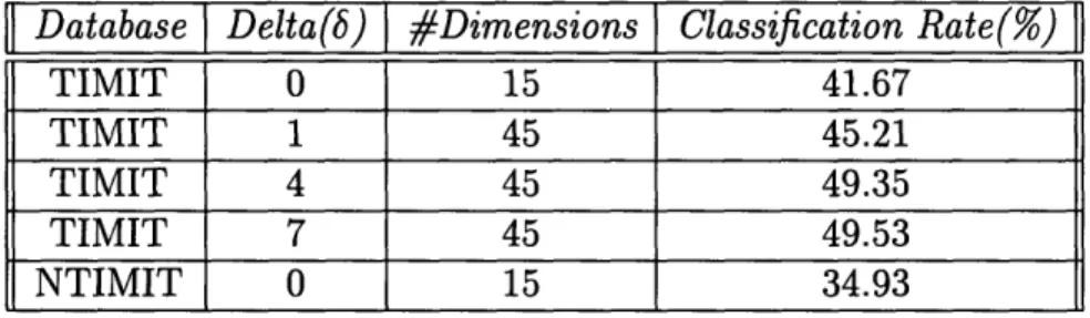
The second set of experiments involved the microsegments as the observations. Ex-actly the same procedure was used as in the case of frame classification, except that other feature vectors were considered. The results are summarized in Table 2.1.

|| Database Delta(b) #Dimensions Classification Rate(%)

TIMIT 0 15 41.67

TIMIT 1 45 45.21

TIMIT 4 45 49.35

TIMIT 7 45 49.53

NTIMIT 0 15 34.93

Table 2.1: Microsegment Classification Results Using Different Deltas

It should be noted at this point that because the boundaries did not exactly coincide with the actual phone boundaries, there are many instances that part of microsegments labelled with a certain phone is not actually part of the phone segment in the correct transcription and this contributes to the error. Comparing these results with the ones for the frame classification, two conclusions can be made. One is that the classification improves from no delta to positive delta. This is because in considering

the microsegments, there is relatively less noise or randomness from one to the next, and the information carried by the delta parameters is enhanced. The second is that the rate improves more as delta is further incremented. This is probably due to an even less randomness from one phone to several phones away from it, and hence a better representation of change.

The next set of experiments take advantage of the context. Given a microsegment, the acoustic vector was augmented by the vectors of the M microsegments before and after it. The number M was varied, and the results shown in Table 2.2. The deltas in Table 2.2 are still with respect to the original microsegment. From the table, one sees that a similar phenomena occurs as in frame classification, that is, that the addition of deltas does not help the classification rate. In this case, the reason is that the delta MFCC's do not correlate with the additional microsegments, hence adding these parameters hinder the performance. It should also be noted that as more microsegments were added, the rate improves. The best result was when there are three additional microsegments on each side and no delta parameters, where a microsegment classification rate of 54.12% was achieved. A phone on average spans 4.4 microsegments, and as we approach this number more and more information about the phone is represented in the feature vector, and this helps the classification rate. It is also interesting to note that adding the delta parameters does not hurt the classification rate much when trained and tested on the NTIMIT database.

As a final experiment on the microsegments, instead of one set of fifteen MFCC averages, three sets are used. A microsegment is divided into three equal subsegments and a fifteen-dimensional MFCC vector is computed per subsegment, giving a total of forty-five acoustic dimensions. This time, no additional microsegments were added on either side, and as the delta was varied, the rate went down and then back up. The results are summarized in Table 2.3.

Database Additional ISegments Delta(6) #Dimensions Classification Rate () on Both Sides (M) TIMIT 1 0 45 49.38 TIMIT 1 1 75 45.69 TIMIT 2 0 75 52.74 TIMIT 2 1 105 49.84 TIMIT 3 0 105 54.12 TIMIT 3 1 135 51.92 TIMIT 3 4 135 51.62 TIMIT 3 7 135 51.42 NTIMIT 1 0 45 39.76 NTIMIT 1 1 75 39.74 NTIMIT 2 0 75 43.80 NTIMIT 2 1 105 43.59 NTIMIT 3 0 105 46.03 NTIMIT 3 1 135 45.66 Table 2.2: Microsegment Microsegments

Classification Results Using Different Deltas and Additional

Database Delta(b) #Dimensions

I

TIMIT 0 45 43.99 TIMIT 1 75 39.26 TIMIT 2 75 43.10 TIMIT 3 75 45.41 TIMIT 4 75 46.98 TIMIT 5 75 48.25 TIMIT 6 75 48.98 TIMIT 7 75 49.15

Microsegment Classification Results Using Different Deltas and Three Table 2.3:

parameters are advantageous in that they embody some representation of change characteristic to phones, and this is evident for larger deltas ( = 6, 7). A small, positive delta, however, incorporates some noisy information and this outweighs the advantages.

2.4.3 Segment Classification

Segment classification is based on the segment phonetic transcription structure de-scribed in Section 2.3.1. Acoustic models were trained on this structure and the models were tested on the same structure of the utterances in the test set. Aside from varying the delta parameter, sometimes three MFCC averages per segment were computed. These represent the beginning (onset), middle and end (offset) of the phone, respectively.

The results are shown in Table 2.4. The best result of 69.0% was achieved when three averages are computed and the delta value was 7. In general, the numbers in Table 2.4 are naturally significantly higher than any of the numbers for microsegment or frame classification. This is because the segments in the segment transcription structure roughly correspond to the whole phones themselves except for some rela-tively small boundary error. Moreover, the results improve again as is increased above 6 = 1 for the same reasons as before, but tapers off after 6 = 7. Likewise, the classification improves as the number of averages computed increases.

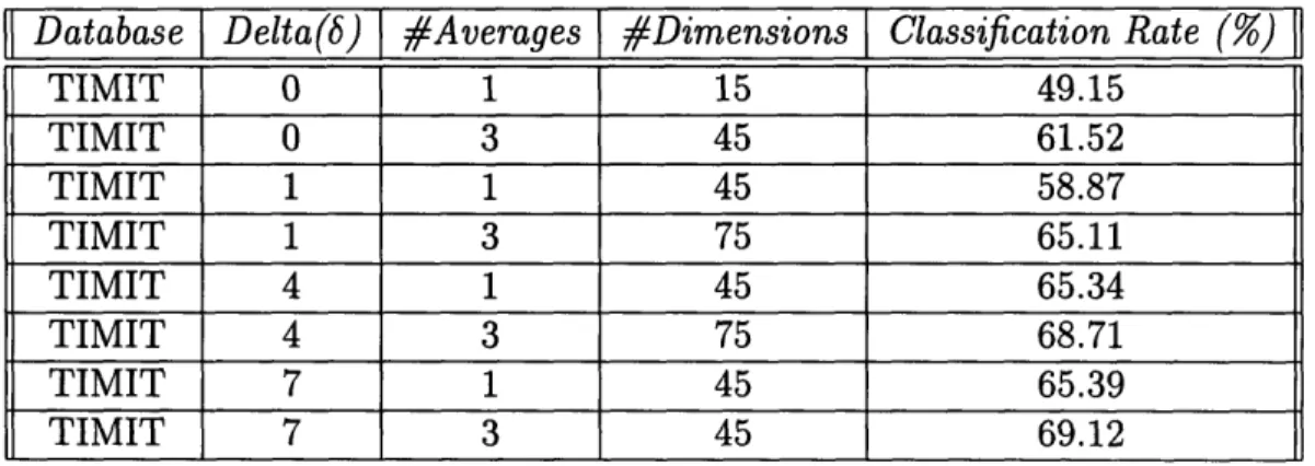
Most classification experiments in the literature are segment-based, and don't propose any boundaries to create the segments. Instead, the exact segments are used in the training and testing algorithm. To simulate the same experiments, the same procedure was performed. The results are shown in Table 2.5, with varying number of averages and deltas.

Database # Averages Delta(6) #Dimensions

I

Table 2.4: Segment Classification With Automatically Aligned Boundaries

Database Delta(6)

#Averages

)

TIMIT 0 1 15 49.15 TIMIT 0 3 45 61.52 TIMIT 1 1 45 58.87 TIMIT 1 3 75 65.11 TIMIT 4 1 45 65.34 TIMIT 4 3 75 68.71 TIMIT 7 1 45 65.39 TIMIT 7 3 45 69.12

better, due to the fact that there are few errors caused by the boundary generation algorithm. The best result of 69.1% was achieved when delta was 7 and three averages per segment were computed. It is also important to note that the improvement in performance caused by an increase in the number of averages computed is more sub-stantial when 6 is lower. The classification rate only counts the number of correctly classified segments, and does not account for near misses. The noisy fluctuations gen-erated from picking small deltas produce a great deal of error where the correct phone classes are very near the top choice, and the increase in the number of averages help increase the probability of the correct phone classes enough to become the top choice. The errors in picking bigger deltas, on the other hand, are probably more serious, where the correct class is relatively farther to the top choice, and the augmentation of acoustic vectors does not help much.

2.5 Summary

Full covariance gaussian acoustic models are trained at the frame, microsegment, and full segment levels, and will be used in implementing the alignment algorithm. In the training of the models, parameters, such as 6 and the number of averages computed per observation, were varied. To determine which parameters resulted with the most accurate models, classification experiments were performed. In general, results improved when 6 values of 4 or higher were used and when more averages were computed per observation.

Chapter 3

Boundary Generation

The boundary generation procedure is described in this chapter. Different acous-tic parameters are experimented with, and the results are evaluated using a set of evaluation criteria.

3.1 Independence of Microsegments

In Chapter 2, the approximation in Equation 2.5 is used for computing the scores of different phone paths. Whenever such a probability is expressed as a product of prob-abilities, there is an assumption of independence between the different observations in the path. Whether such an independence premise is valid or not greatly determines the accuracy of such an approximation.

For frame-based procedures, the independence assumption is severely violated. The average phone duration is approximately 80 ms [6]. Hence, if the present frame is an [s] say, it is highly likely that the succeeding frame will also correspond to an [s]. By grouping frames together into longer segments, one segment will be more likely to be independent from its adjacent segments. The ideal situation is that the signal be divided into the phones themselves. But this is exactly the problem we are

trying to solve! The method of predicting acoustic-phonetic boundaries for phones generally tends to hypothesize many boundaries at intervals of speech where there is significant acoustic change. However, there is usually at most one actual phone boundary at these regions. This is a good start, however, and is in fact the basis of the microsegment-based approach.

In this chapter, the method of boundary selection is described. Acoustic models are then trained from the microsegments formed out of this procedure. Finally, the alignment algorithm chooses the actual phone boundaries from these boundaries and produces an alignment.

3.2 Criteria

One disadvantage of using a microsegment-based approach is that if the boundaries are chosen poorly, certain microsegments overlap with more than one phonetic seg-ment in the correctly aligned transcription, which means that such a microsegseg-ment does not correspond to exactly one phone. Such errors can be prevented if the bound-aries are proposed more frequently. However, the more boundbound-aries that are proposed, the greater the independence assumption is violated, and the less exact the approxi-mation. Hence, there is a tradeoff between lesser boundary errors and lesser approx-imation errors. To maximize such a tradeoff, several measures are used to evaluate the accuracy of the boundaries.

3.2.1 Deletion Rate

The first measure of boundary accuracy is the deletion rate, which is computed in the following way. The proposed boundaries are aligned with the labelled boundaries. For each of the labelled boundary, the closest proposed boundary is found and a

new phonetic transcription is subsequently formed using these "closest" boundaries as the new phonetic boundaries. Occasionally, two or more labelled boundaries will match the same proposed boundary. The phones between these labelled boundaries are consequently deleted in the new phonetic transcription. Such an event is clearly undesirable. Hence, it is imperative the proposed boundaries be chosen such that these deletions are limited.

We can now then define the deletion rate as the ratio of the number of phones deleted over the total number of phones in the original transcription. This quantity is to be calculated for each boundary generation procedure to evaluate it.

3.2.2 Boundary-to-Phoneme Ratio

A second important measure of choice of boundaries is the boundary-to-phoneme ratio. To achieve more independence between the observations, a small boundary-to-phoneme ratio is desired. However, this should not be at the cost of huge deletions and errors. Another advantage of a small ratio is that with fewer boundaries, the number of observations per path in the network is smaller and hence the computation time is smaller. This becomes a big factor when real-time time-alignment algorithms are desired, or if the utterances are longer than normal.

3.2.3 Errors of Boundary Accuracy

Finally, a third measure is the absolute error of the boundaries when compared to the labelled transcriptions. As described earlier, a segment phonetic transcription can be achieved when the closest hypothesized boundary to each labelled phone boundary is found and used as a phoneme boundary for the new transcription. The average absolute difference between these new phone boundaries and the true boundaries can then be calculated.

Such a result tests the accuracy of predicting the exact boundaries. This is crucial since the training and testing algorithms will depend a lot on these new observations. A large error means that there will be erroneous input to the training algorithm. For instance, if the closest boundary to an [s t] sequence is very far to the left of the actual phone boundary between the [s] and the [t], then a significant part of the [s] will be trained as a [t], and this will prove costly in the testing procedure even if the alignment process is sound. Moreover, this closest phonetic transcription symbolizes the best the alignment procedure can do. A large average absolute error implies that a good alignment procedure would not be attainable.

3.3 Parameters

This section describes the parameters used in creating the boundaries, as well as reports the results of the evaluation. The parameters used are mainly acoustic pa-rameters from the input speech signal, as well as some "smoothing" papa-rameters.

3.3.1 Spectral Change and Spectral Derivative

The spectral change of the signal at frame i is computed from the spectrum by taking the euclidean distance of the MFCC vectors between a certain number of offset frames before and after the frame in consideration:

N

SC[i] = (Ai+i[k] - AiAi[k])

_,

_(3.1)

k=1

where SC[i] is the spectral change at time frame i, the quantity Ai[k] is the value of the kth dimension of the acoustic parameter at time frame i, N is the number of components in the acoustic vector and Ai is the offset. The offset used was 2 time

frames (10 ms), so that sudden changes in the spectral change due to noise will not be captured in the process of taking the euclidean distance.

Since the spectral change is a scalar function of time, the usual method of com-puting the spectral derivative is to just take a first difference on the spectral change:

D[i] = SC[i + Ai] - SC[i - Ai].

(3.2)

However, the speech signal is noisy and taking a simple first difference will produce errors. Hence, an alternative method is used [10]. The spectral change function is smoothed by convolving it with a gaussian. The idea is that such a smoothing process will remove much of the noisy variations on the spectral change. Denoting the gaussian function by G, we have

SC'

(SC * G)' = SC * G' + SC' * G.

(3.3)

Since the speech signal is slowly time-varying, the second term on the right is small relative to the first, and we are left with the following expression for the derivative:

SC'

SC * G'.

(3.4)

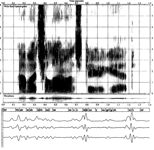
In other words, the derivative of gaussian is computed first then is convolved with the spectral change function. The same method is used in computing further deriva-tives of the spectral change. A plot of the spectral change, spectral derivative and the second derivative of the spectral change for the utterance "How much allowance do you get?" is shown in Figure 3.1. There is generally a peak in the spectral change near phone boundaries. These correspond to positive-to-negative zero crossings of

Time (seconds)

0I0 0.1 0.2 0.3 0.4 0A 0.6 07 (lR 0S 1 a . 14. 1 1 4

0~~~~~~~ ~~ i i I i i i - i i

-Waveform _!

0.0 0.1 0.2 0.3 0.4 0.5 0.6 0.7 0.8 0.9 1.0 1. I 1 .2 1.3 1.4

h* |hhlaw I|mlah It4uh I"a] I a I- I I dC Id ly lux Igllgh tclIt l h#

i:

:.:.:i:

i~. M .

Figure 3.1: Time Plots of Acoustic Parameters

Spectrogram of the utterance "How much allowance do you get?" The plots of the spectral change, spectral derivative and second derivative waveforms are shown below the phonetic

transcription. Wide Ba IS tI p in ' . ' !' ! " "E' _' :

'

L

Ti

pi~~~~~~~~~~~~

_1111Sia

_i

_{1t1.- E |}

_#

_Xi

_i

_l-

_{! ..}

₁₁

S

-- l

,

r

Fr

3.3.2 Peaks in Spectral Change

Phone boundaries are often characterized by a huge spectral change, especially in the case of a closure-stop or a fricative-vowel sequence. Hence, it is natural to look for peaks in the spectral change. In dealing with a continuous waveform, a derivative is taken and the zeroes of this derivative are located and judged as maximas or minimas. Because of the discrete nature of the database, positive-to-negative zero crossings of the spectral derivative are located instead.

3.3.3 Threshold on the Spectral Change

Speech is often accompanied by noise and this noise produces small, random oscil-lations at various parts of the speech signal. Hence, in addition to the zero-crossing of the first spectral derivative, it is necessary to impose further conditions. Without these, there would be too many boundaries hypothesized at areas of the signal where there is no acoustic-phonetic boundary. This would inflate the boundary-to-phoneme ratio without providing much improvement on the deletion rate.

One possible condition is a threshold on the spectral change. This would exclude most of the tiny oscillations from being proposed as boundaries. However, such a threshold cannot be too small either, because a lot of phoneme boundaries are accompanied by very little spectral change, such as in the case of a vowel-semivowel sequence. Clearly, further modifications shall be needed to be able to identify most of these subtle phoneme boundaries without picking too many random boundaries.

3.3.4 Threshold on Second Derivative of Spectral Change

Another possible additional constraint is a threshold on the second derivative of spec-tral change. A positive-to-negative zero-crossing in the derivative of the specspec-tral

change implies a peak in the spectral change. Imposing a threshold on the second derivative in addition to this would only pick boundaries at time frames where the slope of the first derivative zero-crossing is bigger, i.e. the transition from positive to negative in the spectral change is faster, implying a more dramatic change in the spectrum.

3.3.5 Associations on Acoustic Parameters

A variant of the threshold on the second derivative constraint is made by comparing first differences of the spectral change. If the previous first difference is above a certain positive value Ad and the present is below - A d, a boundary can be proposed. This condition corresponds to a significant change in the second derivative, but is more precise on the limits.

3.3.6 Constant Boundaries per Spectral Change

An alternative to having a small threshold above is to impose a larger threshold and then adding various boundaries between the acoustic boundaries. In adding new boundaries, one possibility is to consider the areas where the spectral change is more concentrated. Certainly, phoneme boundaries are more likely to appear at these regions than at areas where the spectral change is close to zero. Moreover, the longer a segment is, the more phone boundaries it probably contains. Taking these two facts into account, it is reasonable to propose adding boundaries at a constant

3.4 Results

In this section the results of different boundary generation algorithms are evaluated. The different parameters described in the previous section are varied, and the resulting deletion rate, boundary-to-phoneme ratio and error rates are compared.

3.4.1 Uniform Boundaries

For baseline performance comparison, the results of using uniform boundaries are evaluated. They are summarized in Table 3.1.

|[ rate(ms. per bdy.) deletions(%) ratio error(ms.) ]

5 0.0 16.16 0 10 0.1 8.08 2 15 0.3 5.40 4 20 1.1 4.06 5 25 1.9 3.25 6 30 3.2 2.72 7 35 4.9 2.34 8 40 6.1 2.05 10 45 8.6 1.83 11 50 11.3 1.65 12

Table 3.1: Results of Uniform Boundaries

The first entry in the table corresponds to a boundary rate of 5 ms per boundary. This is the same as proposing a boundary every frame. As expected, there are no errors or deletions, and the boundary-to-phoneme ratio is high, namely 16.2 bound-aries per phone. The goal of the next boundary experiments is to significantly reduce this number without making the deletion rate or error too big. It is important to note that as the boundary rate is lowered, the deletions go up quickly in the case of uniform boundaries.

3.4.2 Acoustic Boundaries

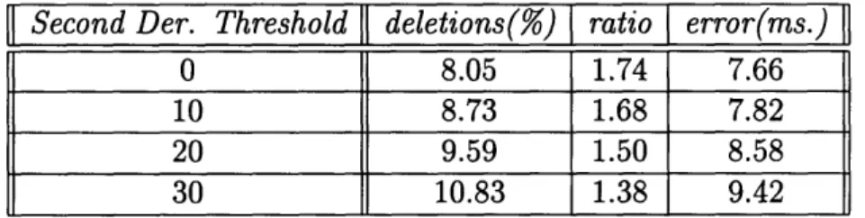
Threshold on Second Derivative

The next experiment involves imposing a second derivative threshold to the spectral change, in addition to a positive-to-negative zero-crossing of the first derivative. The results are summarized in Table 3.2.

. Second Der. Threshold deletions(%) ratio error(ms.)

0 8.05 1.74 7.66

10 8.73 1.68 7.82

20 9.59 1.50 8.58

30 10.83 1.38 9.42

Table 3.2: Varying Threshold on Second Derivative of Spectral Change

These boundaries, however, are not satisfactory by themselves. A no-threshold condition on the second derivative, which means that the only constraints are on the first derivative, gives a very high deletion rate. Clearly, some other way of rewarding more boundaries is needed.

Associations

Another method of proposing acoustic boundaries is by using association on acoustic parameters. Tables 3.3 and 3.4 show the results of using associations on the cepstral and spectral coefficients, respectively, where the threshold is on the second order difference.

|t

Table 3.3: Results of Associations on Cepstral Coefficients

II Threshold on 2nd Ord. Diff. deletions(%) ratio error(ms.)

0.0 3.38 2.808 6.08

3.0 10.30 1.835 11.55

6.0 20.04 1.308 19.39

Table 3.4: Results of Associations on Spectral Coefficients

These results show that associations permit a high deletion rate even though the ratio is low. Furthermore, the tradeoff is bad in relation to uniform boundaries. For instance, a uniform rate of 35 ms produces a deletion rate of 4.9% and a boundary-to-phoneme ratio of 2.34, whereas a 6.0 threshold on the second derivative results in a deletion rate of 5.1% and a ratio of 2.4.

3.4.3 Adding More Boundaries

The above methods by themselves do not produce desired low deletion rates. Clearly, somehow, a new ways of adding boundaries, possibly non-acoustic ones, is needed.

Uniform Boundaries

A simple way of adding boundaries is to put them at a constant rate. For instance, boundaries produced at a constant rate can be added to the set of boundaries derived

by imposing a second derivative threshold. The results of adding uniform boundaries assuming a threshold of 10.0 is presented in Table 3.5.

] rate(ms. per bdy.)

J]

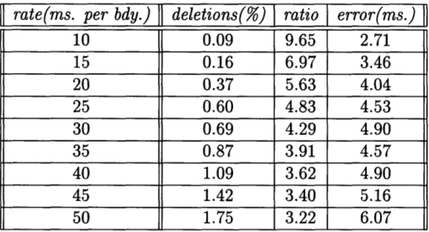
10 0.09 9.65 2.71 15 0.16 6.97 3.46 20 0.37 5.63 4.04 25 0.60 4.83 4.53 30 0.69 4.29 4.90 35 0.87 3.91 4.57 40 1.09 3.62 4.90 45 1.42 3.40 5.16 50 1.75 3.22 6.07

Table 3.5: Results of Adding Uniform Boundaries To Second Derivative Threshold From Table 3.1, a uniform rate of 20 ms per boundary produces a deletion rate of 1.1 percent and a 4.1 boundary-to-phoneme ratio. From Table 3.5, if we add boundaries which are zero-crossings of the first derivative and whose second derivative is above 10, then the deletion rate goes down to a tolerable 0.37 percent, but the boundary-to-phoneme ratio increases only to 5.6. This is clearly a favorable tradeoff. However, the procedure of adding uniform boundaries is a naive way of doing so, since no acoustic information is taken into consideration. Hence there is room for improvement.

Constant Boundaries Per Spectral Change

A more clever way of increasing the boundary ratio is to propose new boundaries where they are more probable to appear. As described before, a way to do this would be to propose constant boundaries per spectral change. Table 3.6 shows the results on adding new boundaries in this manner to those already proposed by imposing a

threshold on spectral change.

Threshold

1

J

0.0 0.0 8.17 1.744 8.45 100.0 0.0 9.18 1.570 9.08 175.0 0.0 13.81 1.189 12.26 175.0 3.0 4.70 1.731 8.46 175.0 5.0 1.85 2.399 6.78 175.0 10.0 0.53 3.688 5.05 175.0 14.0 0.27 4.464 4.50 175.0 25.0 0.20 5.874 3.77 200.0 0.0 15.86 1.110 13.77 200.0 3.0 5.05 1.692 8.79 200.0 5.0 1.93 2.366 6.96 200.0 10.0 0.51 3.660 5.08 200.0 14.0 0.29 4.446 4.51 200.0 25.0 0.20 5.879 3.77 Table 3.6: Threshold

Adding Constant Boundaries Per Spectral Change To Spectral Change

By comparing Tables 3.5 and 3.6, we see that the results of the latter are indeed much better. For instance, in Table 3.5, a uniform rate of 20 ms per boundary produces a deletion rate of 0.37% and a boundary rate of 5.6, whereas a threshold of

175.0 and a rate of 14- 10- 4 _{in Table 3.6 results in a deletion rate of 0.27% and a}

boundary rate of 4.5, an improvement in both categories.

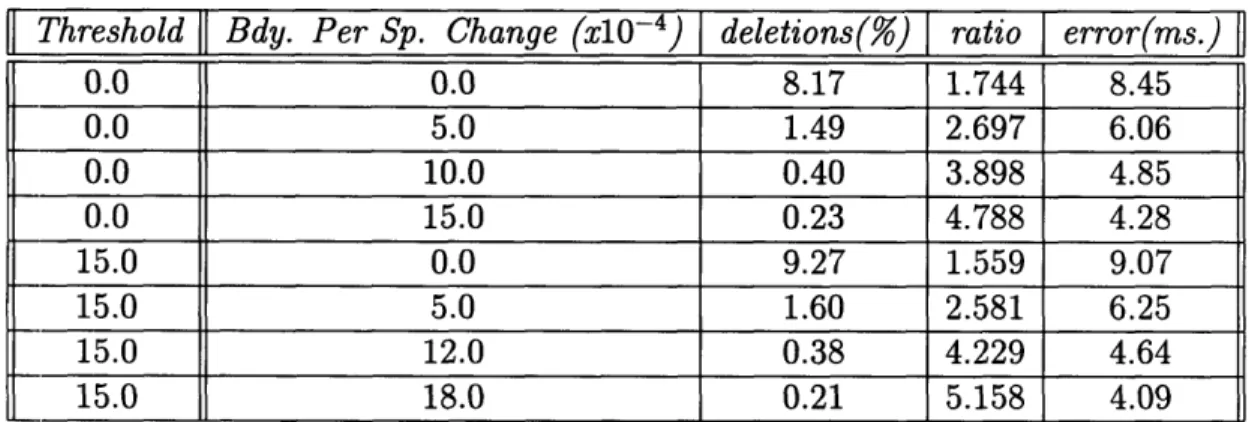
Similar results occur when we add new boundaries to those imposed by a second derivative threshold. They are shown in Table 3.7. These results are in the same order as that of the results in Table 3.6, in terms of the tradeoffs between boundary

I[

Table 3.7: Adding Constant Boundaries Per Spectral Change To Second Derivative Threshold

Minimum Distance Constraint

One obvious problem with adding new boundaries by imposing a constant boundaries per spectral change condition is that there will be a lot of segments that will have a huge concentration of spectral change within some small duration of time, say 25 to 30 ms. After adding new boundaries, there will be too many boundaries proposed in this small segment, by the constant boundaries per spectral change criterion. This often is very unrealistic, since even the shortest phones take up a couple of milliseconds. Hence, a minimum distance between boundaries criteria is proposed at this point, with the belief that this will lessen the number of boundaries without affecting the deletion rate too much. Table 3.8 shows the results of adding the minimum distance constraint on the results of Table 3.6, with the spectral change threshold set at 175.0. Table 3.9 shows the effects on putting minimum boundary distance criteria after imposing a threshold on the second derivative of 10.0.

The tradeoff improved somewhat after imposing the minimum boundary condition to add new boundaries to the ones already proposed by putting a threshold on the spectral change, by comparing Tables 3.6 and 3.8. It worsened somewhat if the initial

Minimum Distance (ms)11 Bdy. Per Sp. Change (x 10- 4_{) deletions(%) | ratio}

[

J

8 16.0 0.24 4.714 4.45

8 14.0 0.29 4.402 4.63

9 16.0 0.25 4.661 4.56

9 14.5 0.32 4.428 4.70

Table 3.8: Adding Minimum Distance Criterion to Spectral Change Threshold of 175.0 and Constant Boundaries

D

8 16.0 0.25 4.831 4.36

8 14.0 0.27 4.530 4.55

9 16.0 0.27 4.775 4.47

9 14.5 0.31 4.475 4.66

Table 3.9: Adding Minimum Distance Criterion to Second 10.0 and Constant Boundaries

Derivative Threshold of

boundaries were chosen by imposing a threshold on the second derivative.

3.5 Selection

From the results of the previous section, the objective now is to pick a set of criteria which will be used in the orthographic alignment.

Comparing the different results of using different set of parameters in the previous section, the tradeoff seems to be the best when a minimum distance constraint is used to add new boundaries to the ones already created when a threshold on the spectral change is used. Hence, the choice of parameters is narrowed down to the set of parameters listed in Table 3.8.