HAL Id: tel-00454616
https://tel.archives-ouvertes.fr/tel-00454616
Submitted on 9 Feb 2010HAL is a multi-disciplinary open access
archive for the deposit and dissemination of sci-entific research documents, whether they are pub-lished or not. The documents may come from teaching and research institutions in France or abroad, or from public or private research centers.
L’archive ouverte pluridisciplinaire HAL, est destinée au dépôt et à la diffusion de documents scientifiques de niveau recherche, publiés ou non, émanant des établissements d’enseignement et de recherche français ou étrangers, des laboratoires publics ou privés.
Ordonnancement de tâches efficace et à complexité
maîtrisée pour des systèmes temps-réel
F. Muhammad
To cite this version:
F. Muhammad. Ordonnancement de tâches efficace et à complexité maîtrisée pour des systèmes temps-réel. Autre. Université Nice Sophia Antipolis, 2009. Français. �tel-00454616�
ECOLE DOCTORALE STIC
SCIENCES ET TECHNOLOGIES DE L’INFORMATION ET DE LA COMMUNICATION
T H E S E
pour obtenir le titre de
Docteur en Sciences
de l’Universit´e de Nice-Sophia Antipolis
Mention: Informatique
pr´esent´ee et soutenue par
Farooq MUHAMMAD
Ordonnancement de Tˆ
aches Efficace et `
a
Complexit´
e Maˆıtris´
ee pour des Syst`
emes Temps
R´
eel
Th`ese dirig´ee par Michel AUGUIN soutenue le 9 Avril 2009
Jury:
M. Pascal Richard Professeur Universit´e de Poitiers Rapporteur M. Yvon Trinquet Professeur Universit´e de Nantes Rapporteur M. Jo¨el Goossens Professeur Universit´e Libre de Bruxelles Examinateur M. Robert de Simone Directeur de Recherche INRIA Pr´esident du Jury M. Michel Auguin Directeur de Recherche CNRS Directeur de Th`ese M. Fabrice Muller Maˆıtre de Conf´erence Universit´e de Nice
Abstract
by Muhammad Farooq
The performance of scheduling algorithm influences the performance of the whole system. Real time scheduling algorithms have theoretical optimal schedulable bounds, but these optimal bounds are achieved at the cost of increased scheduling events (preemptions and migrations of tasks) and high run time complexity of algorithms. We believe that by exploiting parameters of tasks, these algorithms can be made more efficient and cost conscious to increase Quality of Service (QoS) of application.
In first part of thesis, we propose mono-processor scheduling algorithms which increase quality of service of hybrid application by maximizing execution of soft real time tasks, and by providing guarantees to hard real time tasks even in overload situations. Scheduling cost of algorithms is also reduced (in terms of reduced number of preemptions) by taking into account all explicit and implicit parameters of tasks. Reducing scheduling overheads not only increases performance of the scheduler but also minimizes energy consumption of the system. That’s why, we propose to devise a technique embedded with existing DVFS (dynamic voltage and frequency scaling) techniques to minimize the switching points, as switching from one frequency to another steals processor cycles and consumes energy of system.
Multiprocessor scheduling algorithms based on fluid scheduling model (notion of fair-ness), achieve optimal schedulable bounds; but fairness is guaranteed at the cost of un-realistic assumptions, and by increasing preemptions and migrations of tasks to a great extent. An algorithm (ASEDZL) is proposed in this dissertation, which is not based on fluid scheduling model. It not only minimizes preemptions and migrations of tasks but re-laxes the assumptions also due to not being bases on fairness notion. Moreover, ASEDZL is also propose to schedule tasks in hierarchical approach, and it gives better results than other approaches.
par Muhammad Farooq
Les performances des algorithms d’ordonnancement ont un impact direct sur les perfor-mances du syst`eme complet. Les algorithmes d’ordonnancement temps r´eel poss`edent des bornes th´eoriques d’ordonnanabilit´e optimales mais cette optimalit´e est souvent atteinte au prix d’un nombre ´elev´e d’´ev´enements d’ordonnancement `a consid´erer (pr´eemptions et migrations de tˆaches) et d’une complexit´e algorithmique importante. Notre opinion est qu’en exploitant plus efficacement les param`etres des tˆaches il est possible de rendre ces algorithmes plus efficaces et `a coˆut maitris´e, et ce dans le but d’am´eliorer la Qualit´e de Service (QoS) des applications. Nous proposons dans un premier temps des algorithmes d’ordonnancement monoprocesseur qui augmentent la qualit´e de service d’applications hybrides c’est-`a-dire qu’en situation de surcharge, les tˆaches `a contraintes souples ont leur ex´ecution maximis´ee et les ´ech´eances des tˆaches `a contraintes strictes sont garanties. Le coˆut d’ordonnancement de ces algorithmes est aussi r´eduit (nombre de pr´eemptions) par une meilleure exploitation des param`etres implicites et explicites des tˆaches. Cette r´eduction est b´en´efique non seulement pour les performances du syst`eme mais elle agit aussi positivement sur la consommation d’´energie. Aussi nous proposons une technique as-soci´ee `a celle de DVFS (dynamic voltage and frequency scaling) afin de minimiser le nom-bre de changements de points de fonctionnement du fait qu’un changement de fr´equence implique un temps d’inactivit´e du processeur et une consommation d’´energie.
Les algorithmes d’ordonnancement multiprocesseur bas´es sur le mod`ele d’ordonnancement fluide (notion d’´equit´e) atteignent des bornes d’ordonnanabilit´e optimales. Cependant cette ´equit´e n’est garantie qu’au prix d’hypoth`eses irr´ealistes en pratique du fait des nom-bres tr`es ´elev´es de pr´eemptions et de migrations de tˆaches qu’ils induisent. Dans cette th`ese un algorithme est propos´e (ASEDZL) qui n’est pas bas´e sur le mod`ele d’ordonnancement fluide. Il permet non seulement de r´eduire les pr´eemptions et les migrations de tˆaches mais aussi de relˆacher les hypoth`eses impos´ees par ce mod`ele d’ordonnancement. Enfin nous proposons d’utiliser ASEDZL dans une approche d’ordonnancement hi´erarchique ce qui permet d’obtenir de meilleurs r´esultats que les techniques classiques.
Acknowledgements
A journey is easier when we travel together. Interdependence is certainly more valu-able than independence. My entry to graduate school and successful completion of this dissertation and the Ph.D. program are due to the support and help of several people. The following is my attempt at acknowledging everyone I am indebted to.
I am profoundly grateful to my advisors, Fabrice Muller and Michel Auguin, for edu-cating and guiding me over the past few years with great care, enthusiasm, and patience. I am thankful to Michel Auguin for making me consider doing a Ph.D. and taking me under his fold when I decided to go for it. Ever since, it has been an extreme pleasure and a privilege working for Michel and Fabrice and learning from them. They reposed a lot of confidence in me, which, I should confess, was at times overwhelming, and gave me enormous freedom in my work, all the while ensuring that I was making adequate progress. They helped relieve much of the tedium, assuage my apprehensions, boost my self-esteem, and make the whole endeavor a joy by being readily accessible, letting me have their undivided attention most of the time I walked in to their offices, offering sound and timely advice, and when needed, suggesting corrective measures.
I feel honored to have had respected researchers also take the time to serve on my committee. In this regard, thanks are due to Jo¨el Goossens, Pascal Richard, Yvon Trin-quet and Robert De Simone. I am thankful to my entire committee for their feedback on my work and their flexibility in accommodating my requests while scheduling proposals and exams.
In addition, I would like to thank all my colleagues, over the past few years who have helped me become a better researcher. The list would definitely include the following people: Sebastien Icart, Khurram Bhatti, Belaid Ikbel and Zeeshan. Special thanks goes to Sebastien who helped me a lot to improve my french language skills, and special thanks also goes to Belaid ikbel, Khurram Bhatti and Bensaid Siouar whom I spent many enjoyable lunches, dinners and specially caf´e au lait breaks, where we talk about everything other than research stuff. These wonderful breaks really helped me to kick back, relax, cool down a little and gather my energy for hard and tedious work of formal proofs of algorithms. At these times, we used to recharge our spent-up batteries.
I would like to thank to all my friends Najam, Waseem, Naveed, Umer, Khurram, Uzair, Usman, Zeeshan and Rizwaan whose company has always been a great source of encouragement for me. Being in company of such friends, I have enjoyed a lot the period of my thesis. I never felt that I was away from the family. My friends gave me the feelings of being at home.
I would like to give my special thanks to my family whose patient love and prays enabled me to complete this work. I feel a deep sense of gratitude for my father and mother who formed part of my vision and taught me the good things that really matter
I am fortunate to have been blessed with a loving and supportive family, who repose great trust in me. I owe it to my mother and my aunt for instilling in me a passion for learning, and to my father for his pragmatism and for enlivening even mundane things through his wit and sense of humor. I am thankful to my sisters and to my brothers for their affection and prayers. Above all, I am indebted in no small measure to my wife for having endured a lot during the past two years with no complaints. She put up with separation for several months. But for her cooperation, patience, love, and faith, I would not have been able to continue with the Ph.D. program, let alone complete it successfully. I owe almost everything to her and hope to be able to repay her in full in the coming years. Finally, I am thankful to God Almighty for the turn of events that led to this most valuable and rewarding phase of my life. . . .
Abstract iv
Acknowledgements vi
List of Figures xiii
List of Tables xv
Abbreviations xvii
Symbols xix
1 Introduction 1
1.1 Background . . . 1
1.2 Background on Real Time Systems . . . 2
1.3 Real-Time Scheduling Strategies and Classification . . . 3
1.3.1 Feasibility and optimality . . . 3
1.3.2 On-line versus offline scheduling . . . 4
1.3.3 Static versus dynamic priorities . . . 4
1.4 Real-time Scheduling on Multiprocessors . . . 5
1.4.1 Multiprocessor Scheduling Approaches . . . 5
1.4.1.1 Partitioning . . . 5
1.4.1.2 Global scheduling . . . 6
1.4.1.3 Two-level hybrid scheduling. . . 6
1.5 Low-Power Embedded Operating Systems . . . 6
1.5.1 DVFS . . . 7
1.6 Self Adaptive scheduling . . . 9
1.7 Contributions . . . 9
1.7.1 RUF scheduling algorithm . . . 10
1.7.2 Power Efficiency . . . 10
1.7.3 ASEDZL scheduling Algorithm . . . 11
1.7.4 Hierarchical Scheduling Algorithms. . . 11
1.7.5 ÆTHER: Self-adaptive Middleware. . . 12
1.8 Organization . . . 12 ix
Contents x
2 Real Urgency First Scheduling Algorithm 27
2.1 Introduction. . . 27
2.2 Approach Description . . . 29
2.2.1 Dynamic Slack . . . 29
2.2.2 Virtual task . . . 29
2.2.3 Dummy Task . . . 30
2.2.4 Management of non critical tasks . . . 31
2.2.4.1 Selection of Non Critical task . . . 31
2.2.4.2 Inserting Points of Non Critical Task . . . 32
2.2.5 Multiple Virtual tasks . . . 32
2.3 Feasibility Analysis For Critical Tasks . . . 33
2.4 Algorithm . . . 35
2.5 Experimental Results. . . 36
2.6 Conclusions . . . 39
3 Power Efficient Middleware 41 3.1 Introduction. . . 41
3.2 Minimizing number of preemptions . . . 43
3.2.1 Algorithm EEDF . . . 44
3.2.1.1 Static Computation . . . 47
3.2.1.2 Dynamic Computations . . . 48
3.2.1.3 Feasibility Analysis . . . 50
3.2.1.4 Experimental Results of EEDF . . . 51
3.2.2 Algorithm ERM . . . 52
3.2.2.1 Feasibility Analysis of RM . . . 53
3.2.2.2 Experimental Results of ERM . . . 55
3.2.3 Chained Preemptions . . . 56
3.3 Minimizing switching Points and Preemptions . . . 57
3.3.1 Identification of switching points . . . 57
3.3.2 Calculation of the frequency slow down (α) factor . . . 59
3.3.3 Processor Idling . . . 59
3.3.3.1 Minimizing Processor Idle Time . . . 59
3.3.3.2 Gradual Increase in Frequency . . . 60
3.3.3.3 Self adaptive approach . . . 62
3.3.3.4 Experimental Results of EDVFS . . . 62
3.4 Conclusion . . . 62
4 Efficient and Optimal Multiprocessor Scheduling for Real Time Tasks 65 4.1 Introduction. . . 65
4.2 EDF based Scheduling Algorithms and their Utilization Bounds. . . 67
4.2.1 Dhall’s Effect . . . 68
4.2.2 Accumulative Effect . . . 69
4.2.2.1 Single Processor Case . . . 69
4.2.2.2 Multiprocessor Case . . . 70
4.3 Multiprocessor ASEDZL Scheduling . . . 70
4.3.1 T askQueue . . . 71
4.3.3 Virtual Deadline and Local Execution Time . . . 72
4.3.4 Priority Order of Tasks . . . 73
4.4 Comparison of EDZL With ASEDZL . . . 75
4.5 Properties of ASEDZL Algorithm . . . 76
4.5.1 Not Based on Basic Time Quanta . . . 76
4.5.2 Notion of Fairness . . . 77
4.5.2.1 Pfair Fairness . . . 77
4.5.2.2 LLREF Fairness . . . 77
4.5.2.3 ASEDZL Fairness . . . 78
4.5.3 Minimum Active Tasks Between two Release Instants . . . 79
4.5.4 Anticipation of Laxities of M TEDF Tasks . . . 79
4.6 Optimality of ASEDZL . . . 79
4.6.1 U (τ ) at Release Instants Ri . . . 80
4.6.2 No Idle Time on Processor . . . 82
4.6.2.1 2D Bin Packing . . . 82
4.6.2.2 Minimum Number of Ready Tasks: . . . 83
4.6.3 No More than M Urgent tasks . . . 84
4.7 Complete Example . . . 85
4.8 Performance Evaluation . . . 87
4.9 Algorithm Overhead . . . 88
4.10 Conclusions . . . 89
5 Hierarchical Scheduling Algorithm 91 5.1 Introduction. . . 91
5.2 Weight Bound Relation between supertask and component tasks for guar-anteed real time constraints . . . 92
5.2.1 Background . . . 93
5.2.1.1 Pfair Scheduling Algorithm . . . 93
5.2.1.2 Local Scheduler and parameters of supertask . . . 96
5.2.2 Schedulability Conditions . . . 97
5.2.3 Schedulability Conditions for Component tasks . . . 98
5.2.3.1 Necessary Condition . . . 99
5.2.3.2 Number/Length of window task . . . 100
5.2.3.3 Embedded task Periods . . . 104
5.2.3.4 Exemptions . . . 104 5.2.4 Reweighting Rules . . . 105 5.2.5 Results . . . 106 5.2.6 Partitioning of tasks . . . 107 5.2.6.1 Next Fit (NF) . . . 107 5.2.6.2 First Fit (FF) . . . 107 5.2.6.3 Best Fit (BF) . . . 107
5.3 Hierarchical Scheduling Based on Slack Anticipation Approach . . . 109
5.3.1 Approach Description . . . 109
5.3.1.1 Local Scheduler . . . 109
5.3.1.2 Local Release instants . . . 110
5.3.1.3 Supertask . . . 110
Contents xii
5.3.1.5 Release instants for ASEDZL . . . 111
5.3.2 Schedulability Analysis . . . 112
5.3.2.1 Schedulability analysis for global and supertasks . . . 112
5.3.2.2 Schedulability of Partitioned tasks . . . 112
5.4 Conclusions . . . 116
6 Conclusions 119 6.1 Summary . . . 119
6.2 Future Work . . . 122
A ÆTHER: Self adaptive Resource Management Middleware for Selfopti-mizing Resources 129 A.1 Introduction. . . 129
A.1.1 Definition Of The Problem . . . 130
A.2 ÆTHER Architectural Model . . . 131
A.3 Application Model . . . 132
A.3.1 Task Structure . . . 133
A.3.1.1 Worst Case Execution Time . . . 134
A.3.1.2 Best Case Execution Time . . . 134
A.3.2 Self Adaptive Task Structuring . . . 135
A.3.2.1 Dedicated SANE for a Task. . . 135
A.3.2.2 Optimized SANE for Family of µT s of a Task . . . 135
A.4 Resource Allocation and Scheduling . . . 136
A.4.1 Wasted Resource Utilization . . . 136
A.4.1.1 Homogenous Concurrent µthreads . . . 136
A.4.1.2 Heterogeneous Concurrent µthreads . . . 137
A.5 Minimum Resources for Each Task . . . 138
A.5.1 Task Preemption . . . 138
A.6 Algorithm . . . 139
A.7 Schedulability . . . 140
A.8 Conclusions . . . 140
A.9 Acknowledgment . . . 141
B Dynamic Scheduling of Global and Local Tasks in Their Reserved Slots143 B.1 Algorithm Description . . . 144 B.1.1 Local Scheduler. . . 144 B.1.2 Global Scheduler . . . 145 B.2 Schedulability Analysis. . . 145 B.3 Runtime Optimizations . . . 146 B.4 Comparison . . . 147 Bibliography 149
2.1 Approach Description . . . 30
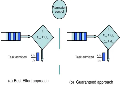
2.2 Two types of Admission Control . . . 31
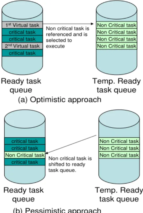
2.3 Comparison of variants of approach. . . 33
2.4 execution scenario of non critical task. . . 35
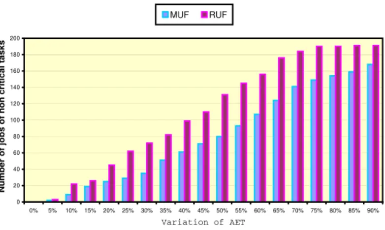
2.5 Execution of non critical tasks over hyper-period of critical tasks . . . 37
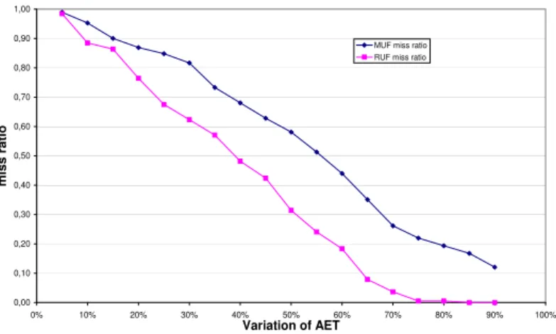
2.6 Miss ratio of non critical tasks over hyper-period . . . 38
2.7 Success ratio of RUF vs MUF . . . 38
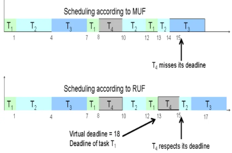
2.8 Example comparing MUF and RUF. . . 39
3.1 task having higher frequency can preempt low frequent tasks . . . 44
3.2 complete Example . . . 46
3.3 Calculation of N P Zj . . . 48
3.4 Comparison of Number of Preemptions. . . 52
3.5 EEDF static Vs EEDF dynamic . . . 52
3.6 Comparison of Number of Preemptions. . . 55
3.7 Phenomena of chained preemptions in EDF scheduling . . . 56
3.8 Phenomena of chained preemptions in EEDF scheduling . . . 56
3.9 Comparison of two approaches . . . 58
3.10 Approach Description (Flow Diagram) . . . 58
3.11 Idle time on the processor . . . 59
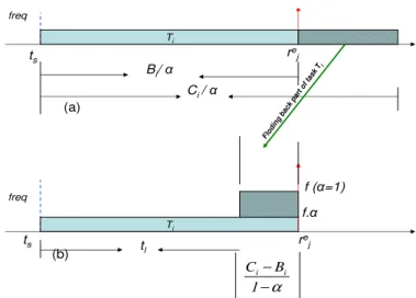
3.12 Folding execution time . . . 60
3.13 Gradual increase in frequency of the processor. . . 61
3.14 EDVFS Vs DVFS . . . 63
4.1 Dhall’s Effect . . . 68
4.2 EDZL removes dhall’s effect . . . 69
4.3 Tasks sorted according to EDF . . . 71
4.4 Release instants Ri associated with tasks and interval length . . . 72
4.5 ASEDZL scheduling Algorithm Description . . . 75
4.6 Comparison of EDF with EDZL . . . 75
4.7 Comparison of EDZL with ASEDZL . . . 76
4.8 Fairness ensured at each instant. . . 77
4.9 Fairness ensured at each release instant . . . 78
4.10 Fairness ensured at deadline boundaries . . . 78
4.11 2D Bin Packing . . . 83
4.12 Optimality proof . . . 85
4.13 : Illustration of Algorithm by Complete Example . . . 87
4.14 T askQueue at different Release Instants . . . 87 xiii
List of Figures xiv
4.15 Comparison of ASEDZL algorithm with LLREF . . . 88
4.16 Comparison of ASEDZL algorithm with EDZL algorithm . . . 89
5.1 Hierarchical scheduler . . . 93
5.2 The Pfair windows of the first job (or 8 window tasks) of a task Ti with weight 8/11 in a Pfair-scheduled system. . . 95
5.3 Scheduling of tasks on two processors by a Pfair scheduler . . . 97
5.4 Scheduling of supertask and component tasks. . . 98
5.5 Number of windows in an interval. . . 102
5.6 Window tasks defined for supertask. . . 102
5.7 Schedulability condition for component task. . . 103
5.8 Demonstration of scheduling of supertasks and component tasks. . . 106
5.9 Local T askQueues . . . 110
5.10 Interaction between Global and Local scheduler. . . 112
5.11 Maximum demand of tasks on processor . . . 114
5.12 Demonstrating Example . . . 115
5.13 Execution of Local Tasks . . . 116
A.1 Self Adaptive Networked Entity (SANE) . . . 131
A.2 SANE processor composed of SANE Elements. . . 132
A.3 SANE Assemblies. . . 132
A.4 Representation of a task . . . 133
A.5 Execution time of task . . . 134
A.6 Varied task structure . . . 135
A.7 Restructuring of Task self adaptively . . . 136
A.8 Wasted Resource Utilization. . . 137
A.9 Recalculation of Rm . . . 140
B.1 Under-utilization distribution at runtime. . . 144
B.2 Distribution of under-utilization between release instants . . . 145
2.1 Task Parameters . . . 38
3.1 Task Parameters . . . 46
4.1 Task Parameters . . . 86
5.1 Task Parameters . . . 96
5.2 Comparison of Our proposed Reweighting rules with those proposed by Anand et al.. . . 107
5.3 Task Parameters . . . 114
EDF Earliest Deadline First
EEDF Enhanced Earliest Deadline First
RM Rate Monotonic
ERM Enhanced Rate Monotonic LLF Least Laxity First
CASH CApacity SHaring MUF Maximum Urgency First
QRAM QoS Resource Allocation Model Pfair Proportionate Fair
LLREF Least Local Remaining Eexecution First EDZL Earliest Deadline until Zero Laxity
ASEDZL Anticipating Slack Earliest Deadline until Zero Laxity DVFS Dynamic Voltage and Frequency Scaling
EDVFS Enhanced Dynamic Voltage and Frequency Scaling NPZ No Preemption Zone
τ set of tasks
τpar set of partitioned tasks
τg set of global tasks
τi set of tasks partitioned on processor Π i
τr(t) represent set of ready task at time t
HP hyper period of n tasks Ti task Ti
Ci worst case execution time of task Ti
Cirem(t) remaining execution time of Ti at time t
Bi best case execution time of Ti
Pi period of Ti
di absolute deadline of task Ti
dremi (t) remaining time to deadline of Ti
µi utilization or weight of task Ti
U (τ ) sum of utilizations of all tasks
Π set of identical processors in an architecture Πj jth processor
Rk kth release instant in a schedule
Rjk local release instant on processor Πj
Txj supertask on processor Πj
Introduction
1.1
Background
The distinguishing characteristic of a real-time system in comparison to a non-real-time system is the inclusion of timing requirements in its specification. That is, the correctness of a real-time system depends not only on logically correct segments of code that produce logically correct results, but also on executing the code segments and producing correct results within specific time frames. Thus, a real-time system is often said to possess dual notions of correctness, logical and temporal. Process control systems, which multiplex several control-law computations, radar signal-processing and tracking systems, and air traffic control systems are some examples of real-time systems.
Timing requirements and constraints in real-time systems are commonly specified as deadlines within which activities should complete execution. Consider a radar tracking system as an example. To track targets of interest, the radar system performs the following high-level activities or tasks: sends radio pulses towards the targets, receives and processes the echo signals returned to determine the position and velocity of the objects or sources that reflected the pulses, and finally, associates the sources with targets and updates their trajectories. For effective tracking, each of the above tasks should be invoked repeatedly at a frequency that depends on the distance, velocity, and the importance of the targets, and each invocation should complete execution within a specified time or deadline.
Another characteristic of a real-time system is that it should be predictable. Pre-dictability means that it should be possible to show, demonstrate, or prove that require-ments are always met subject to any assumptions made, such as on workloads.
Based on the cost of failure associated with not meeting them, timing constraints in real-time systems can be classified broadly as either hard or soft. A hard real-time constraint is one whose violation can lead to disastrous consequences such as loss of life or a significant loss to property. Industrial process-control systems and robots, controllers for automotive systems, and air-traffic controllers are some examples of systems with hard
Chapter 1. Introduction and Background 2
real-time constraints. In contrast, a soft real-time constraint is less critical; hence, soft real-time constraints can be violated. However, such violations are not desirable, either, as they may lead to degraded quality of service, and it is often the case that the extent of violation be bounded. Multimedia systems and virtual-reality systems are some examples of systems with soft real-time constraints.
There are several emerging real-time applications that are very complex and have high computational requirements. Examples of such systems include automatic tracking sys-tems and tele-presence syssys-tems. These applications have timing constraints that are used to ensure high system fidelity and responsiveness, and may also be crucial for correct-ness in certain applications such as tele-surgery. Also, their processing requirements may easily exceed the capacity of a single processor, and a multiprocessor may be necessary to achieve an effective implementation. In addition, multiprocessors are, generally, more cost-effective than a single processor of the same capacity because the cost (monetary) of a k-processor system is significantly less than that of a processor that is k times as fast (if a processor of that speed is indeed available).
The above observations clearly underscore the growing importance of scheduling algo-rithms in real-time systems. In this dissertation, we focus on several fundamental issues pertaining to the scheduling of real-time tasks on mono-processor as well as on multipro-cessor architecture. Before discussing the contributions of this dissertation in more detail, we briefly describe some basic concepts pertaining to real-time systems.
1.2
Background on Real Time Systems
A real-time system is typically composed of several (sequential) processes with timing constraints. We refer to these processes as tasks and set of these tasks is represented by τ = {T1, T2, ..., Tn}. In most real-time systems, tasks are recurrent, i.e., each task
is invoked repeatedly. The periodic task model of Liu and Layland [48] provides the simplest notion of a recurrent task. Each periodic task Ti is characterized by a phase
φi, a period Pi, a relative deadline di, and an execution requirement Ci (Ci < di). The
best case execution time is represented by Bi. Such a task is invoked every Pi time units,
with its first invocation occurring at time φi. We refer to each invocation of a task as a
job/instance, and the corresponding time of invocation as the job’s release time. Thus, the relative deadline parameter is used to specify the timing constraints of the jobs of a periodic task. Unless stated otherwise, we assume that relative deadline of a periodic task equals its period. In other words, each job must complete before the release of the next job of the same task. We define few run time parameters of a task such as Crem
i (t) which represents the remaining execution time of task Ti at time t defined as
Cirem(t) = Ci− Cicompleted(t) where Cicompleted(t) represents the completed fraction of task
The remaining time to deadline of a task Ti is defined as dremi (t) = di− t. A dynamic
parameter of tasks Ti is AETi which represents the actual execution time of task Ti.
Each task Ti has its own laxity Li defined as:
Li = Pi− Ci
and laxity at time t is defined as:
Li(t) = dremi (t) − Cirem(t)
A periodic task system in which all tasks have a phase of zero is called a synchronous periodic task system, and we have considered synchronous task system in this dissertation unless stated otherwise. Let HP represents the hyper period of all tasks which is the least common multiple of periods of all n tasks. The weight or utilization of a task Ti, denoted
µi, is the ratio of its execution requirement to its period. We use the terms weight and
utilization interchangeably in this dissertation. µi = Ci/Pi. The weight (or utilization)
of a task system is the sum of the weights of all tasks in the system. Offloading factor of a task Ti, denoted by Oi, represents the percentage of a processor that can be used to
execute tasks other than Ti, and Oi is the ratio of task’s laxity to its period (i.e., Li/Pi).
In this dissertation, we assume that all tasks are synchronous and preemptive, i.e., a task can be interrupted during its execution and resumed later from the same point. Unless stated otherwise, we assume that the overhead of a preemption is zero. We further assume that all tasks are independent, i.e., the execution of a task is not affected by the execution of other tasks. In particular, we assume that tasks do not share any resources other than the processor, and that they do not self-suspend during execution.
1.3
Real-Time Scheduling Strategies and Classification
In general, real time scheduling algorithm assigns a priority to each job, and on an M -processor system, schedules for execution the M jobs with the highest priorities at any instant.1.3.1 Feasibility and optimality
A periodic task system τ is feasible on processing platform if and only if for every possible real-time instance there exists a way to meet all deadlines. A feasibility test for a class of task systems is specified by giving a condition that is necessary and sufficient to ensure that any task system in that class is feasible.
The algorithm that is used to schedule tasks (i.e., allocate processor time to tasks) is referred to as a scheduling algorithm. A task system τ is said to be schedulable by
Chapter 1. Introduction and Background 4
algorithm A if A can guarantee the deadlines of all jobs of every task in τ . A condition under which all task systems within a class of task systems are schedulable by A is referred to as a schedulability test for A for that class of task systems. A scheduling algorithm is defined as optimal for a class of task systems if its schedulability condition is identical to the feasibility condition for that class.
1.3.2 On-line versus offline scheduling
In offline scheduling, the entire schedule for a task system (up to a certain time such as the the least common multiple (LCM) of all task periods) is pre-computed before the system actually runs; the actual run-time scheduling is done using a table based on this pre-computed schedule. On the other hand, an on-line scheduler selects a job for scheduling without any knowledge of future job releases. (Note that an on-line scheduling algorithm can also be used to produce an offline schedule.) Clearly, offline scheduling is more efficient at run-time; however, this efficiency comes at the cost of flexibility. In order to produce an off-line schedule, it is necessary to know the exact release times for all jobs in the system. However, such knowledge may not be available in many systems, in particular, those consisting of sporadic tasks, or periodic tasks with unknown phases. Even if such knowledge is available, then it may be impractical to store the entire precomputed schedule (e.g., if the LCM of the task periods is very large). On the other hand, on-line schedulers need to be very efficient, and hence, may need to make sub-optimal scheduling decisions, resulting in schedulability loss.
1.3.3 Static versus dynamic priorities
Most scheduling algorithms are priority-based: they assign priorities to the tasks or jobs in the system and these priorities are used to select a job for execution whenever scheduling decisions are made. A priority-based scheduling algorithm can determine task or job priorities in different ways.
A scheduling algorithm is called a static-priority algorithm if there is a unique priority associated with each task, and all jobs generated by a task have the priority associated with that task. Thus, if task Ti has higher priority than task Tj, then whenever both
have active jobs, Ti’s job has higher priority than Tj’s job. An example of a scheduling
algorithm that uses static priorities is the rate-monotonic (RM) algorithm [48]. The RM algorithm assigns higher priority to tasks with shorter periods.
Dynamic-priority algorithms allow more flexibility in priority assignments; a task’s priority may vary across jobs or even within a job. An example of a scheduling algorithm that uses dynamic priorities is the earliest-deadline-first (EDF) algorithm [48]. EDF assigns higher priority to jobs with earlier deadlines, and has been shown to be optimal for scheduling periodic and sporadic tasks on uniprocessors [48,54]. The least laxity- first
(LLF) algorithm [54] is also an example of a dynamic-priority algorithm that is optimal on uniprocessors. As its name suggests, under LLF, jobs with lower laxity are assigned higher priority.
1.4
Real-time Scheduling on Multiprocessors
In this subsection, we consider multiprocessor scheduling in some details.1.4.1 Multiprocessor Scheduling Approaches
Scheduling of tasks on multiprocessor systems is typically solved using two different meth-ods based on how tasks are assigned to the processors at run-time, namely partitioning and non-partitioning. In the partitioning-based method, all instances of a task are ex-ecuted on the same processor, which is determined before run-time by a partitioning algorithm. In a non partitioning method, any instance of a task can be executed on a different processor, or even be preempted and moved to a different processor, before it is completed.
1.4.1.1 Partitioning
Under partitioning, the set of tasks is statically partitioned among processors, that is, each task is assigned to a unique processor upon which all its jobs execute. Each processor is associated with a separate instance of a uniprocessor scheduler for scheduling the tasks assigned to it and a separate local ready queue for storing its ready jobs. In other words, the priority space associated with each processor is local to it. The different per-processor schedulers may all be based on the same scheduling algorithm or use different ones. The algorithm that partitions the tasks among processors should ensure that for each processor, the sum of the utilizations of tasks assigned to it is at the most utilization bound of its scheduler.
Partitioning method have several advantages over non partitioning methods [4, 46,
58, 59, 71]. Firstly, the scheduling overhead associated with a partitioning method is lower than the overhead associated with a non-partitioning method. Secondly, partition-ing methods allow us to apply well-known uniprocessor schedulpartition-ing algorithms on each processor. Thirdly and most importantly, each processor could use resources dedicated to it i.e., distributed memory etc. The last mentioned aspect improves the performance of the system a lot, and in most cases it proves the partitioning method to be better than its counterpart. Optimal assignment of tasks to processors is known to be NP-hard, which is major drawback of partitioning method.
Chapter 1. Introduction and Background 6
1.4.1.2 Global scheduling
In contrast to partitioning, under global scheduling, a single, system-wide, priority space is considered, and a global ready queue is used for storing ready jobs. At any instant, at most M ready jobs with the highest priority (in the global priority space) execute on the M processors. No restrictions are imposed on where a task may execute; not only can different jobs of a task execute on different processors, but a given job can execute on different processors at different times.
In contrast, the non-partitioning method has received much less attention [44,49,51,
52], mainly because it is believed to suffer from scheduling and implementation-related shortcomings, also because it lacks support for more advanced system models, such as the management of shared resources. The other important factor that makes this approach of less interest is the use of a shared memory which introduces the bottleneck for system scalability. On the better side, schedulability bounds are much better than its counterpart.
1.4.1.3 Two-level hybrid scheduling
Some algorithms do not strictly fall under either of the above two categories, but have elements of both. For example, algorithms for scheduling systems in which some tasks cannot migrate and have to be bound to a particular processor, while others can migrate, follow a mixed strategy. In general, scheduling under a mixed strategy is at two levels: at the first level, a single, global scheduler determines the processor that each job should be assigned to using global rules, while at the second level, the jobs assigned to individual processors are scheduled by per-processor schedulers using local priorities. Several variants of this general model and other types of hybrid scheduling are also possible. Typically, the global scheduler is associated with a global queue of ready, but unassigned jobs, and the per-processor schedulers with queues that are local to them.
1.5
Low-Power Embedded Operating Systems
The tremendous increase in demand for many battery-operated computing devices evi-dences the need for power-aware computing. As a new dimension of CPU computing, the goal of power-aware CPU scheduling is to dynamically adjust hardware to adapt to the expected performance of the current workload so that a system can efficiently save power, lengthening its battery life for useful work in the future. In addition to traditional low − power designs for the highest performance delivery, the new concept focuses on en-abling hardware-software collaboration to scale down power and performance in hardware whenever the system performance can be relaxed.
Power-saving State Control (PSC) and Dynamic Voltage and Frequency Scaling (DVFS) are promising examples of power-aware techniques developed in hardware. Power-saving
states are like operating knobs of a device, as they consume much less power and sup-port only partial functionalities compared to the regular active operating mode. With the prevailing power-saving trend, power states have been ubiquitously supported in pro-cessors, disks, RDRAM memory chips, wireless network cards, LCD displays, etc. Com-mon power-saving states include standby (clock-gating), retention (clock-gating with just enough reduced supply voltage to save the logic contents of circuits), and power-down (power-gating) modes. Some devices provide specific power-states that offer more energy-efficient operating options such as the control of the back light in LCD displays and the control of the modulation scheme and transmission rate in wireless network cards.
DVFS techniques are deployed in many commercial processors such as Transmeta’s Crusoe, Intel’s XScale processors and Texas Instruments OMAP3430. Due to the fact that dynamic power in CMOS circuits has a quadratic dependency on the supply volt-age, lowering the supply voltage is an effective way to reduce power. However, this voltage reduction also adversely affects the system performance through increasing delay. Therefore, efficient DVFS algorithms must maintain the performance delivery required by applications.
No matter how advanced power-aware strategies in circuit designs and hardware drivers may become, they must be integrated with applications and the operating systems, and knowledge of the applications intents is essential. Advanced Configuration and Power Interface (ACPI) [23] is an open industry specification that establishes interfaces for the operating system (OS) to directly configure power states and supply voltages on each individual device. ACPI was developed by Hewlett-Packard, Intel, Microsoft, Phoenix and Toshiba. The operating system thus can customize energy policies to maintain the quality of service required by applications and assign proper operating modes to each device at runtime.
1.5.1 DVFS
The field of dynamic voltage and frequency scaling (DVFS) is currently the focus of a great deal of power-aware research. This is due to the fact that the dynamic power consumption of CMOS circuits [28,72] is given by:
P W = βCLVDD2 f (1.1)
where β is the average activity factor, CL is the average load capacitance, VDD is
the supply voltage and f is the operating frequency. Since the power has a quadratic dependency on the supply voltage, scaling the voltage down is the most effective way to minimize energy. However, lowering the supply voltage can also adversely affect the system performance due to increasing delay. The maximum operating speed is a direct
Chapter 1. Introduction and Background 8
consequence of the supply voltage given by:
f = K(VDD− Vth)
β
VDD
(1.2) where K is a constant specific to a given technology, Vth is the threshold voltage and
β is the velocity saturation index, 1 ≤ β ≤ 2
DVFS algorithms that target real-time systems instead assume the knowledge of timing constraints of real-time tasks which are specified by users or application developers in < C, P, d > tuple. Pillai and Shin [35] proposed a wide-ranging class of voltage scaling algorithms for real-time systems. In their static voltage scaling algorithm, instead of running tasks with different speeds, only one system frequency is determined and used. Their operating frequency is determined by equally scaling all tasks to complete the lowest-priority task as late as possible. This turns out to be pessimistic. Since the amount of preemption by high-priority tasks is not uniformly distributed when there are multiple task periods, a task can encounter less preemption relative to its own computation and save more energy if it completes earlier than its deadline.
Aydin et al. [10] proposed the optimal static voltage scaling algorithm using the solution in reward-based scheduling. Their approach assigns a single operating frequency for each task and focuses on the EDF scheduling policy. DVFS effectively minimizes the energy consumption but cost of voltage/frequency switch is high in some architectures. One example for these systems is the Compaq IPAQ, which needs at least 20 milliseconds to synchronize SDRAM timing after switching voltage (frequency). Voltage switch cost on ARM11 implemented in the IMX31 architecture of Freescale is about 4 milliseconds). For such systems, switching voltage at every point when task finishes its execution before its worst case execution time is unacceptable. In this dissertation, we focus on minimizing the voltage/frequency switching points but not at the cost of wasting unused processor cycles.
Until now, We have considered a task model where tasks can execute only on one processor at a time, but with the invent of new programming paradigms like MPI, open-MP and Snet we are able to execute more than one threads of a task in parallel on a multiprocessor or on multi-core (chip multiprocessing) systems even on FPGAs as well. The degree of parallelism at different levels of a task is different which must be taken care of while reserving resources for tasks. This can be tackled by allocating resources dynamically, but if architecture can improve its processing capabilities at run time to well suit the varying demands of application, then there is a need to schedule tasks by a self adaptive approach. Moreover, if demands of applications changes at run time, then we are left with no solution of scheduling such task but self adaptive scheduling technique.
1.6
Self Adaptive scheduling
Scheduling of adaptively parallel jobs for which the number of processors which can be used without waste changes during runtime can be achieved by scheduler where number of processors allocated to tasks are static. Parallelism at each level of task is not same and task can self-optimize itself during runtime as well, thus offering different degree of parallelism at different than calculated before. So, there is a need to schedule tasks dynamically and adaptively. Most prior work on task scheduling for multi-tasked jobs deals with nonadaptive scheduling, where the scheduler allots a fixed number of processors to the job for its entire lifetime. For jobs whose parallelism is unknown in advance and which may change during execution, this strategy may waste processor cycles, because a job with low parallelism may be allotted more processors than it can productively use. Moreover, in a multiprogrammed environment, nonadaptive scheduling may not allow a new job to start, because existing jobs may already be using most of the processors. With adaptive scheduling, the job scheduler can change the number of processors allotted to a job while the job is executing. Thus, new jobs can enter the system, because the job scheduler can simply recruit processors from the already executing jobs and allot them to the newly arrived tasks.
1.7
Contributions
The main thesis supported by this dissertation is the following.
Real time scheduling algorithms have schedulable bounds equal to the capacity of architec-ture (based on some assumptions) but can be made more efficient by minimize scheduling overheads to increase QoS (Quality of Service) of application, and this efficiency is at-tained by taking into account task’s implicit run time parameters. Moreover, the schedula-ble bounds equal to capacity of architecture can be achieved by relaxing these assumptions.
In the following subsections, we describe the contributions of this dissertation in more detail. In addition to optimal schedulable bounds (which is clearly important), efficiency is essential in several of the emerging real-time applications to improve QoS of application and to minimize power consumption of the system. The objective is to propose scheduling algorithms, which have very low run time complexity in terms of algorithmic complexity and number of the invocations during execution of tasks i.e., reduced scheduling events. Moreover, algorithms, which increase the number of tasks executed for given time by exploiting runtime parameters of tasks, are also considered more efficient, as QoS of application is directly related with number of tasks executed over a given period. In this dissertation, we address the efficiency issues by introducing significant modifications to existing scheduling algorithms to minimize scheduling events, cost of one scheduling event and to improve QoS of application (briefly described in Section 1.7.1). We also address the
Chapter 1. Introduction and Background 10
issues related to power efficiency of architecture and provide schemes to minimize power consumption of the system without compromising on the schedulability bound (Section 1.7.2). In case of multiprocessor system, schedulable bounds are achieved by making unrealistic assumptions about application, for which runtime complexity, preemptions and migration of tasks are quiet high. We handle this issue of runtime complexity and preemptions (and migrations) on multiprocessor architecture, and devise technique which relaxes these assumptions and reduces preemptions to a great extent(Section 1.7.3). We also study hybrid scheduling algorithms, and present three approaches which have optimal schedulable bounds and reduced cost(section1.7.4).
1.7.1 RUF scheduling algorithm
If task set is composed of critical and non critical tasks, and overall load of all tasks is greater than 100%, then there is a need to devise a technique where all critical tasks are guaranteed to meet their deadlines, and execution of non critical tasks is maximized as well. Existing algorithms (EDF,MUF,CASH) either do not provides guarantees to critical tasks in transient overload situation, or minimize the execution of non critical tasks. We propose to exploit the run time parameters of tasks i.e., time slot of processor available at runtime, Ci− AETi which is the difference beteween actual and worst case execution
of task, not only to provide guarantees to critical tasks but to maximize the execution of non critical tasks also. To handle this issue, a new scheduling algorithm called RUF (Real Urgency First) is proposed with objective to increase the QoS of application. We define an admission control mechanism for non critical tasks to maximize their execution but without compromising on deadline guarantees of critical tasks. This admission of non critical task at time t depends upon the run time parameters of all those critcal tasks which have finsihed their execution until t. We illustrate the prinicple through an example and demonstrate experimentally that proposed algorithm incurs less preemptions than all existing algorithms in terms of maximizing executions of critical tasks.
1.7.2 Power Efficiency
In case of mono processor system, real time scheduling algorithms have optimal schedula-ble bounds but they have either high run time complexity or incurs a lot of preemptions of tasks (increased scheduling events). These increased preemptions and high runtime com-plexity of scheduling algorithms not only decrease the schedulable bounds (practically), but also increase energy consumption of the system. These algorithms do not exploit all implicit and runtime parameters of a task to minimize these overheads and energy of the system . Laxity is an implicit parameter of task, which provides certain level of flexibility to scheduler. Scheduler can exploit this flexibility to relax certain rules of scheduling algorithm that can help to minimize scheduling overheads and preemptions of tasks. We
propose to exploit this implicit parameter to define an algorithm which significantly re-duces preemptions of tasks. Two variants of the approach are proposed to exploit run time parameters of tasks to minimize preemptions, one is static and the other is dynamic. Moreover, we also propose to exploit these parameter both in case of dynamic and static priority scheduling algorithms i.e., for EDF and RM.
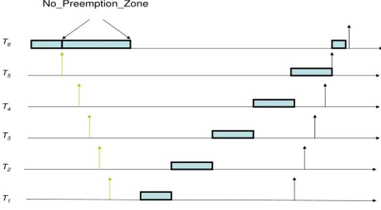
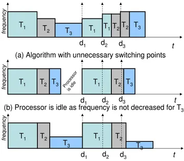
We also observed that preemptions of tasks are directly related with load of processor and minimizing number of preemptions is beneficial to reduce the energy consumption of the system. However, DVFS algorithms minimize the frequency of processor to decrease power consumption which has its adverse effect on increasing the number of preemptions. We propose an algorithm, where frequency of the processor is decreased only at those instants when it does not have its impact on the number of preemptions. Moreover, it is also ensured that switching points of frequency (where frequency of processor is changed) are also minimized, as changing from one level of frequency to another level consumes energy and processor time.
1.7.3 ASEDZL scheduling Algorithm
In case of multiprocessor systems, scheduling algorithms have been proposed which are optimal but they are based on fluid schedule model or fairness notion. Algorithms based on notion of fairness, increase scheduling overheads (preemptions and scheduler invocations) to such a great extent that sometimes they are impractical. To minimize these scheduling overheads, we propose a scheduling algorithm which is not based on fluid schedule (or fairness notion).
We propose an algorithm called Anticipating Slack Earliest Deadline First until zero laxity(ASEDZL). According to this algorithm, tasks are not allocated processor time in proportion to their weights. Tasks are selected to execute between two consecutive task’s release instants and tasks with the earliest deadlines are ensured to execute on all processors until next release instant. This proposed algorithm provides better results in terms of minimum number of preemptions and migrations of tasks for not being based on fluid scheduling model. We illustrate the principle through couple of examples, and we also demonstrate through simulation results that it performs better than all those algorithms which have schedulable bound equal to capacity of the architecture.
1.7.4 Hierarchical Scheduling Algorithms
Hierarchical scheduling or hybrid scheduling algorithms guarantees better results than partitioning or global scheduling algorithms in case of distributed shared memory archi-tecture but very few hybrid scheduling algorithms are proposed which have schedulable bound equal to number of processors (with some assumptions, detailed in chapter 5). Moir et al. [53] proposed a technique of supertasking approach for hybrid scheduling algorithm,
Chapter 1. Introduction and Background 12
where Pfair scheduling algorithm is used as global scheduler, but it was required to de-fine weight bound condition between local tasks (partitioned tasks) and its corresponding supertask to achieve optimal schedulable bound, we establish that condition. We also propose to use ASEDZL scheduling algorithm as global scheduler, as it does not impose any condition on weights of supertask and local tasks. We compare, analytically, this proposed algorithm with existing approaches to illustrate that it promises better results. A novel hybrid scheduling algorithm is also proposed, where time slots are reserved for execution of local and global tasks.
1.7.5 ÆTHER: Self-adaptive Middleware
Self-adaptive scheduling algorithms deal with tasks for which degree of parallelism is calculated statically, and resources are allocated dynamically to cope different degree of parallelism at different levels of sequential execution of a task to minimize wastage. These algorithms also deal with dynamic creation and deletion of tasks, but they don’t deal where tasks can self-optimize at run time and due to this self-optimization, degree of parallelism at different levels of sequential execution of a task may differ from that of calculated statically. Moreover, architecture can also self-optimize to execute parallel threads on one resource more efficiently than executing each thread on separate resource. These run time optimizations of architecture and application requires an intelligent self-adaptive resource management mechanism that can tackle all these run time variations. We propose a self-adaptive scheduling model, which takes care of all these run time optimization of tasks and architecture to schedule tasks on resources, and provide deadline guarantees to real time tasks.
1.8
Organization
In Chapter 2, we exploit the runtime parameter of a task which is Ci−AETito improve the
QoS of an application, while in Chapter 3, we propose to work on both implicit and run-time parameters of a task which are its laxity and release run-times respectively to minimize the preemptions of tasks in schedule. In Chapter 4, we aim to take care of both explicit and implicit parameters of a task i.e., Ci, Pi and Li, to propose an optimal global
mul-tiprocessor scheduling algorithm. Chapter 5 covers the proposed hierarchical scheduling algorithms, where we have presented results using Pfair and ASEDZL scheduling algo-rithm as a global scheduler. In each chapter, related state of art is also presented before describing our work and results. In the last chapter, we summarize our contributions and discuss directions for future research.
1.1 G´
en´
eralit´
es
La diff´erence principale entre un syst`eme temps r´eel par rapport `a un syst`eme transaction-nel ou mˆeme hautes performances est l’introduction de conditions temporelles dans ses sp´ecifications. En d’autres termes, un syst`eme temps r´eel est correct non seulement si le code applicatif est logiquement correct et produit des r´esultats logiquement corrects, mais ´
egalement si ces r´esultats sont produits dans des intervalles de temps pr´ecis. Ainsi, un syst`eme temps r´eel poss`ede des notions duales d’exactitude relatives aux aspects logique et temporel. Les syst`emes de contrˆole de processus qui multiplexent plusieurs calculs de lois de commande tels du traitement de signal radar et de suivi de cibles dans un syst`eme de contrˆole de trafic a´erien est un exemple de syst`emes temps r´eel.
Les conditions et les contraintes temporelles dans les syst`emes temps r´eel sont g´en´ erale-ment sp´ecifi´ees sous forme d’´ech´eances avant lesquelles les activit´es du syst`eme doivent terminer leurs ex´ecutions. Consid´erons comme exemple un syst`eme de suivi radar. Pour suivre des cibles d’int´erˆet, le syst`eme radar effectue les activit´es ou tˆaches suivantes : envoi des impulsions par radio vers les cibles, r´eception et traitement des signaux d’´echo re¸cus pour d´eterminer la position et la vitesse des objets ou des sources qui ont renvoy´e les impulsions, et enfin association des sources aux cibles et mise `a jour de leurs trajectoires. Pour un suivi efficace, chacune des tˆaches ci-dessus doit ˆetre ex´ecut´ee p´eriodiquement `a une fr´equence qui d´epend de la distance, de la vitesse, et de l’importance des cibles et, `a chaque invocation, doit ex´ecuter la tˆache dans un d´elai ou suivant une ´ech´eance sp´ecifique. Une autre caract´eristique d’un syst`eme temps r´eel est qu’il devrait ˆetre pr´evisible. La pr´evisibilit´e signifie qu’il devrait ˆetre possible de montrer ou de prouver que les exigences des tˆaches sont toujours satisfaites quelles que soient les hypoth`eses faites, comme la charge de calcul sur le ou les processeurs.
En fonction des cons´equences induites par un non respect des exigences des tˆaches, les contraintes de temps sont g´en´eralement class´ees comme dures ou souples. Une con-trainte de temps dure correspond par exemple `a ´ech´eance dont la violation peut entrainer des cons´equences d´esastreuses tels que des risques pour des vies humaines ou des d´egˆats mat´eriels importants. Des syst`emes de contrˆole de proc´ed´es industriels, des contrˆoleurs
Chapter 1. Introduction 14
embarqu´es dans l’automobile ou des syst`emes de contrˆole a´erien en a´eronautique sont au-tant d’exemples de syst`emes soumis `a des contraintes de temps r´eel dur. Par comparaison, un syst`eme temps r´eel souple poss`ede des contraintes moins critiques, le d´epassement de contraintes souples est ainsi possible. Cependant, ces d´epassements ne sont en g´en´eral pas souhaitables du fait que la qualit´e de service du syst`eme se d´egrade avec le nom-bre de d´epassements observ´es et par cons´equent, ce nombre est g´en´eralement born´e. Les syst`emes multim´edia ou de r´ealit´e virtuelle sont des exemples de syst`emes `a contraintes de temps souples.
Il existe des applications ´emergentes `a la fois temps r´eel et de grande complexit´e algo-rithmique. Des exemples sont les syst`emes de suivi automatique de cibles et les syst`emes de t´el´e-surveillance. Ces applications ont des contraintes temporelles qui visent `a produire une grande r´eactivit´e du syst`eme et peuvent ˆetre aussi n´ecessaires pour assurer un com-portement correct voire crucial dans certaines applications telle que la t´el´e-chirurgie. En outre, leurs besoins de traitement peuvent facilement d´epasser la capacit´e de calcul d’un simple processeur et dans ce cas, un syst`eme multiprocesseur peut ˆetre n´ecessaire pour r´ealiser une ex´ecution efficace de l’application. Par ailleurs, les architectures multipro-cesseurs peuvent ˆetre plus rentables qu’un processeur unique de mˆeme capacit´e de calcul du fait que le coˆut d’un syst`eme `a k-processeurs peut ˆetre moins ´elev´e que celui d’un processeur k fois plus rapide (dans l’hypoth`ese o`u un processeur de cette performance est en effet disponible).
Ces observations soulignent l’importance croissante des architectures multiprocesseurs dans les syst`emes temps r´eel et celle des algorithmes d’ordonnancement de tˆaches adapt´es `
a ces architectures. Dans cette th`ese, nous nous concentrons sur plusieurs points centraux relatifs `a cette probl´ematique. Avant d’introduire les contributions d´evelopp´ees dans la th`ese, nous d´ecrivons bri`evement quelques concepts de base concernant les syst`emes temps r´eel.
1.2 Les syst`
emes temps r´
eel : concepts de base
Un syst`eme temps r´eel se compose typiquement de plusieurs processus (s´equentiels) munis de contraintes temporelles. Nous appelons ces processus des tˆaches. Dans la plupart des syst`emes temps r´eel, les tˆaches sont r´ecurrentes, c’est `a dire que chaque tˆache est appel´ee r´ep´etitivement tant que le syst`eme fonctionne. Le mod`ele de tˆaches p´eriodiques introduit par Liu et Layland [48] fournit la notion la plus simple d’une tˆache r´ecurrente. Chaque tˆache p´eriodique Tiest caract´eris´ee par une phase φi, une p´eriode Pi, une ´ech´eance relative
di, et un temps d’ex´ecution pire cas Ci (Ci ≤ di). La quantit´e Bi repr´esente le temps
d’ex´ecution minimum d’une tˆache. Une telle tˆache est activ´ee toutes les Pi unit´es de
Nous d´esignons par le terme ”travail” chaque invocation d’une tˆache, et l’instant cor-respondant `a une invocation d’une tˆache comme instant d’activation du travail. Ainsi, le param`etre relatif `a l’´ech´eance est employ´e pour sp´ecifier les contraintes temporelles des travaux d’une tˆache p´eriodique. Sauf indication contraire, nous supposons que l’´ech´eance relative d’une tˆache p´eriodique est ´egale `a sa p´eriode. En d’autres termes, chaque tra-vail doit terminer son ex´ecution avant l’activation du prochain travail de la mˆeme tˆache. Nous d´efinissons les diff´erents param`etres d’ex´ecution d’une tˆache suivants. Le param`etre Cirem(t) repr´esente la dur´ee d’ex´ecution restante de la tˆache Ti `a l’instant t d´efinie par
Cirem(t) = Ci− Cicompleted(t) o`u C
completed
i (t) repr´esente la fraction du temps d’ex´ecution
r´ealis´ee de la tˆache Ti jusqu’`a l’instant t. Le param`etre Birem(t) repr´esente le temps
d’ex´ecution minimum restant `a l’instant t. La quantit´e dremi (t) = di− t, d´efinit la dur´ee
restante `a l’´ech´eance de Ti. Le param`etre AETi associ´e `a une tˆache Ti repr´esente le
temps d’ex´ecution effectif d’un travail relatif `a une invocation de cette tˆache, il s’agit d’un param`etre dynamique.
A chaque tˆache Ti on associe une latence Li d´efinie par:
Li = Pi− Ci
La latence d’une tˆache Ti `a l’instant t est d´efinie par :
Li(t) = dremi (t) − Cirem(t)
Un syst`eme de tˆaches p´eriodiques dans lequel toutes les tˆaches ont une phase nulle est un syst`eme de tˆaches p´eriodiques synchrones. Sauf indications contraires, nous consid´erons dans la suite de la th`ese des tˆaches de cette nature. Le terme HP d´esigne l’hyperp´eriode de toutes les tˆaches c’est `a dire le plus petit commun multiple des p´eriodes des n tˆaches. Le poids ou l’utilisation d’une tˆache Ti, not´e µi, est le rapport entre son temps d’ex´ecution
pire cas et sa p´eriode (Ci/Pi). Le poids d’une tˆache d´etermine la fraction de temps d’un
processeur que la tˆache requiert pour son ex´ecution pendant sa p´eriode. Le poids d’un syst`eme de tˆaches est la somme des poids de toutes les tˆaches dans le syst`eme.
Nous supposons que toutes les tˆaches sont pr´eemptives, c’est `a dire qu’une tˆache peut ˆ
etre interrompue pendant son ex´ecution et reprise plus tard `a partir du mˆeme point d’arrˆet. Nous supposons que les coˆuts en temps li´es `a la pr´eemption d’une tˆache sont n´egligeables. Nous supposons ´egalement que toutes les tˆaches sont ind´ependantes, en d’autres termes, l’ex´ecution d’une tˆache n’est pas conditionn´ee par un ou des r´esultats fournis par d’autres tˆaches. En particulier, nous supposons que les tˆaches ne partagent aucune ressource autre que le processeur, et qu’elles ne s’auto-suspendent pas pendant leur ex´ecution.
Chapter 1. Introduction 16
1.3 Les strat´
egies d’ordonnancement temps r´
eel et leur
clas-sification
G´en´eralement, un algorithme d’ordonnancement temps r´eel affecte une priorit´e `a chaque travail, et dans le cas d’un syst`eme `a M processeurs, planifie l’ex´ecution des M travaux ayant les priorit´es les plus ´elev´ees `a chaque instant.
1.3.1 1.3.1 Faisabilit´e et optimalit´e
Un syst`eme de tˆaches p´eriodiques est faisable sur une architecture mono ou multipro-cesseur si et seulement si pour chaque invocation de chaque tˆache, il est possible de re-specter toutes les ´ech´eances. Un test de faisabilit´e pour une classe de syst`emes de tˆaches est d´efini comme une condition n´ecessaire et suffisante `a v´erifier pour s’assurer que tout syst`eme de tˆaches dans cette classe soit faisable.
Un algorithme employ´e pour planifier des tˆaches (c’est `a dire, allouer un temps du pro-cesseur aux tˆaches) est d´esign´e sous le nom d’algorithme d’ordonnancement. Un syst`eme de tˆaches τ est ordonnan¸cable par l’algorithme A si A peut garantir les ´ech´eances de tous les travaux de chaque tˆache dans τ . Une condition suivant laquelle tous les syst`emes de tˆaches dans une classe sont ordonnan¸cables par A est un test d’ordonnan¸cabilit´e pour A pour cette classe de syst`emes de tˆaches. Un algorithme d’ordonnancement est consid´er´e comme optimal pour une classe de syst`emes de tˆaches si sa condition d’ordonnan¸cabilit´e est identique `a la condition de faisabilit´e pour cette classe.
1.3.2 Ordonnancement en ligne et hors ligne
Dans un ordonnancement hors ligne, l’ordonnancement complet d’un syst`eme de tˆaches (jusqu’`a un temps d´efini par l’hyperp´eriode des tˆaches) est pr´e-calcul´e avant que le syst`eme ne soit ex´ecut´e r´eellement; l’ordonnancement des ex´ecutions des tˆaches est effectu´e en utilisant une table bas´ee sur cet ordonnancement pr´e-calcul´e. Afin de produire un ordon-nancement hors ligne, il est n´ecessaire de connaˆıtre les temps exacts d’activation de tous les travaux du syst`eme. Cependant, une telle connaissance n’est pas toujours disponible, en particulier pour ceux qui contiennent des tˆaches sporadiques, ou p´eriodiques avec des phases inconnues. Mˆeme si une telle connaissance ´etait disponible, alors il peut ˆetre irr´ealiste de m´emoriser l’ordonnancement complet dans le cas o`u le PPCM des p´eriodes des tˆaches est tr`es grand. Par ailleurs, un ordonnanceur en ligne choisit un travail `a ordon-nancer sans aucune connaissance des activations des travaux futurs. On peut noter qu’un algorithme d’ordonnancement en ligne peut ˆetre ´egalement employ´e pour produire un or-donnancement hors ligne. De mani`ere ´evidente, un ordonnancement hors ligne est plus efficace `a l’ex´ecution qu’un ordonnancement en ligne, cependant la flexibilit´e est r´eduite
dans le cas hors ligne. Les ordonnanceurs en ligne doivent ˆetre efficaces, mais peuvent avoir `a prendre des d´ecisions d’ordonnancement sous-optimales.
1.3.3 Priorit´es Statiques et Dynamiques
La plupart des algorithmes d’ordonnancement est bas´ee sur le principe de priorit´e: ils attribuent des priorit´es aux tˆaches ou aux travaux dans le syst`eme et ces priorit´es sont utilis´ees pour s´electionner un travail `a ex´ecuter en fonction des d´ecisions d’ordonnancement prises. Un algorithme d’ordonnancement bas´e sur les priorit´es peut d´eterminer les priorit´es des tˆaches ou de travaux de diff´erentes mani`eres. Un algorithme d’ordonnancement est `a priorit´es statiques si une priorit´e unique est associ´ee `a chaque tˆache, et tous les travaux issus d’une mˆeme tˆache poss`edent la priorit´e li´ee `a cette tˆache. Ainsi, si la tˆache Ti a
une priorit´e plus ´elev´ee que la tˆache Tj , alors lorsque toutes les deux deviennent actives,
le travail de Ti aura une priorit´e plus ´elev´ee que celui de Tj . Un exemple d’algorithme
d’ordonnancement bas´e sur des priorit´es statiques est l’algorithme Rate-Monotonic (RM) [48]. L’algorithme RM affecte les priorit´es les plus ´elev´ees aux tˆaches ayant des p´eriodes les plus courtes. Les algorithmes `a priorit´e dynamique permettent une plus grande flexibilit´e dans l’attribution des priorit´es aux tˆaches. La priorit´e d’une tˆache peut varier entre les travaux ou mˆeme au sein du mˆeme travail. Un exemple d’algorithme d’ordonnancement `
a priorit´es dynamiques est l’algorithme Earliest Deadline First (EDF) [48]. Cet algo-rithme associe une priorit´e plus ´elev´ees aux travaux ayant des ´ech´eances plus proches. Il est prouv´e que cet algorithme est optimal pour ordonnancer des tˆaches p´eriodiques et sporadiques sur une architecture monoprocesseur [48, 54]. L’algorithme Least Laxity-First (LLF) [54] est ´egalement un exemple d’algorithme `a priorit´es dynamiques - il est ´
egalement optimal pour des architectures monoprocesseurs. Comme son nom le sugg`ere, sous LLF, les travaux ayant des laxit´es les plus faibles ont les priorit´es les plus ´elev´ees.
1.4 Ordonnancement temps-r´
eel multiprocesseur
Dans cette ce paragraphe, nous d´etaillons des approches d’ordonnancement d´evelopp´ees dans le cas multiprocesseur.
1.4.1 Approches d’ordonnancements multiprocesseurs
Deux approches traditionnelles consid´er´ees pour l’ordonnancement sur architectures mul-tiprocesseurs sont l’ordonnancement avec partitionnement et l’ordonnancement global.
1.4.1.1 Approche par partitionnement
Sous le terme ordonnancement par partitionnement, il faut consid´erer un ensemble de tˆaches (statiquement) partitionn´ees sur les processeurs. Chaque tˆache est allou´ee `a un
Chapter 1. Introduction 18
processeur unique sur lequel elle s’ex´ecute. Chaque processeur poss`ede son propre or-donnanceur qui lui permet de s´electionner localement les tˆaches `a ex´ecuter parmi celles qui lui ont ´et´e attribu´ees. Il poss`ede ´egalement une file locale des tˆaches dans laquelle sont rang´es les travaux prˆets `a ˆetre ex´ecut´es. En d’autres termes, l’espace des priorit´es affect´e `a chaque tˆache est local `a chaque processeur. De plus, les ordonnanceurs de chaque processeur peuvent ˆetre tous bas´es sur le mˆeme algorithme d’ordonnancement ou chacun peut utiliser son propre algorithme. Enfin, le partitionnement des tˆaches sur l’ensemble des processeurs doit s’assurer que pour chaque processeur, la somme des utilisations des tˆaches allou´ees au processeur est au plus ´egale `a la limite d’utilisation possible de son ordonnanceur.
1.4.1.2 L’approche par ordonnancement global
Par opposition `a l’ordonnancement par partitionnement, l’ordonnancement global utilise un espace unique pour les priorit´es. Il n’existe qu’une seule file globale des tˆaches prˆetes. A chaque instant, les M tˆaches prˆetes qui poss`edent les plus grandes priorit´es dans l’espace global des priorit´es s’ex´ecutent sur les M processeurs. Aucune restriction n’est impos´ee ici sur le choix du processeur qui ex´ecute une tˆache prˆete et s´electionn´ee. En particulier, l’ex´ecution d’une tˆache peut ˆetre amen´ee `a migrer d’un processeur `a un autre en fonction des d´ecisions d’ordonnancement.
1.4.1.3 L’ordonnancement hybride `a deux niveaux
Certains algorithmes d’ordonnancement ne r´epondent pas strictement aux deux approches pr´esent´ees ci-dessus mais utilisent les deux approches `a la fois. Par exemple, des algo-rithmes dans lesquelles certaines tˆaches ne peuvent pas migrer et doivent donc ˆetre af-fect´ees `a un processeur sp´ecifique alors que d’autres tˆaches ont la possibilit´e de migrer. Ces algorithmes suivent une strat´egie mixte. En g´en´eral, un ordonnancement bas´e sur une strat´egie mixte est r´ealis´e sur deux niveaux. Au premier niveau, un ordonnanceur global et unique d´etermine le processeur sur lequel les tˆaches devraient ˆetre allou´ees et ce en fonction de r`egles globales. Au second niveau, les tˆaches allou´ees `a un processeur sont ordonnanc´ees localement en fonction de priorit´es locales. Plusieurs variantes de ce mod`ele g´en´eral ainsi que d’autres types d’ordonnancements hybrides sont ´egalement possibles.
1.5 Syst`
emes d’exploitation embarqu´
es pour la gestion de
l’´
energie
L’accroissement important de la demande pour l’ex´ecution d’applications sur les syst`emes autonomes (sur batterie) met en ´evidence un besoin d’ex´ecuter des applications en ten-ant compte de la consommation d’´energie engendr´ee. Avec les nouvelles g´en´erations de