HAL Id: hal-01868735
https://hal.archives-ouvertes.fr/hal-01868735
Submitted on 7 Sep 2018
HAL is a multi-disciplinary open access
archive for the deposit and dissemination of
sci-entific research documents, whether they are
pub-lished or not. The documents may come from
teaching and research institutions in France or
abroad, or from public or private research centers.
L’archive ouverte pluridisciplinaire HAL, est
destinée au dépôt et à la diffusion de documents
scientifiques de niveau recherche, publiés ou non,
émanant des établissements d’enseignement et de
recherche français ou étrangers, des laboratoires
publics ou privés.
Optimizing deep video representation to match brain
activity
Hugo Richard, Ana Pinho, Bertrand Thirion, Guillaume Charpiat
To cite this version:
Hugo Richard, Ana Pinho, Bertrand Thirion, Guillaume Charpiat. Optimizing deep video
represen-tation to match brain activity. CCN 2018 - Conference on Cognitive Compurepresen-tational Neuroscience,
Sep 2018, Philadelphia, United States. �hal-01868735�
Optimizing deep video representation to match brain activity
Hugo Richard ([email protected])
PARIETAL Team, INRIA, 1 Rue Honor d’Estienne d’Orves, 91120 Palaiseau, France
Ana Lu´ısa Pinho ([email protected])
PARIETAL Team, INRIA, 1 Rue Honor d’Estienne d’Orves, 91120 Palaiseau, France
Bertrand Thirion ([email protected])
PARIETAL Team, INRIA, 1 Rue Honor d’Estienne d’Orves, 91120 Palaiseau, France
Guillaume Charpiat ([email protected])
TAU team, INRIA, LRI, Paris-Sud University, France
Abstract
The comparison of observed brain activity with the statis-tics generated by artificial intelligence systems is useful to probe brain functional organization under ecological condi-tions. Here we study fMRI activity in ten subjects watching color natural movies and compute deep representations of these movies with an architecture that relies on optical flow and image content. The association of activity in visual ar-eas with the different layers of the deep architecture displays complexity-related contrasts across visual areas and reveals a striking foveal/peripheral dichotomy.
Keywords: deep learning; video encoding; brain mapping;
Introduction
The understanding of brain functional architecture has long been driven by subtractive reasoning approaches, in which the activation patterns associated with different experimen-tal conditions presented in event-related or block designs are contrasted in order to yield condition-specific maps (Poline & Brett, 2012). A more ecological way of stimulating sub-jects consists in presenting complex continuous stimuli that are much more similar to every-day cognitive experiences.
The analysis of the ensuing complex stimulation streams proceeds by extracting relevant features from the stimuli and correlating the occurrence of these features with brain ac-tivity recorded simultaneously with the presentation of the stimuli. The analysis of video streams has been carried in (Eickenberg, Gramfort, Varoquaux, & Thirion, 2017) or (G ¨uc¸l ¨u & van Gerven, 2015) using a deep convolutional network trained for image classification. More recently, (G ¨uc¸l ¨u & van Gerven, 2017) has used a deep neural network trained for ac-tion recogniac-tion to analyze video streams.
Like (G ¨uc¸l ¨u & van Gerven, 2017), we use a deep neural network trained for action recognition to extract video features and train a linear model to predict brain activity from these fea-tures. In contrast, our study is not restricted to dorsal stream visual areas but involves the whole brain, and the deep neural network we use is pretrained on the largest action recognition dataset available (Kay et al., 2017).
From the different layers of the deep neural networks, we build video representations that allow us to segregate (1) oc-cipital and lateral areas of the visual cortex (reproducing the
results of (G ¨uc¸l ¨u & van Gerven, 2015)) and (2) foveal and pe-ripheric areas of the visual cortex. We also introduce an effi-cient spatial compression scheme for deep video features that allows us to speed up the training of our predictive algorithm. We show that our compression scheme outperforms PCA by a large margin.
Methods
Deep video representationWe use a deep neural network trained for action recognition to build deep representations of the Berkeley Video stimuli (Nishimoto et al., 2011). This material consists of more than four hours of color natural movies built by mixing video blocks
of5-15seconds in a random fashion.
The deep network we use is called Temporal Segment Net-work (TSN) (Wang et al., 2016). Following an idea introduced in 2014 (Simonyan & Zisserman, 2014) it was intended to mimic the dorsal and ventral stream by separately process-ing raw frames and optical flow fields. We chose TSN for our experiments because it uses a much larger number of layers than the original network (which results in higher accuracy in action recognition) and that a version of TSN pretrained on Kinetics – a massive video dataset (300 000 unique video clips) with 400 different classes all describing a human and at least 400 videos per class – is publicly available. The network is trained to recognize human actions such as slack-lining, skateboarding, massaging feet, dancing zumba and dining.
The version of TSN we use in our experiments is based on Inception v3 (Szegedy, Vanhoucke, Ioffe, Shlens, & Wo-jna, 2016) for both streams where small networks are used as building blocks of the main large network (Lin, Chen, & Yan, 2013). Each stream in the TSN Network is composed of more than 40 convolution layers and a fully connected layer. The activities after the last layer represent the probability of be-longing to each action class.
Feature extraction
The raw frames encode information about pixels, and flow
fields encode information about pixels displacements.
Al-though flow fields and raw frames streams do not precisely disentangle spatial content and motion information in videos,
we may expect that the raw frames stream better represent local spatial features while the flow fields stream more effi-ciently convey dynamic information. Following (Eickenberg et al., 2017) we consider that the activation statistics in the first layers (the ones closer to those of the input) have a low level of abstraction, whereas the last layers (closer to the labels) rep-resent high-level information. Therefore each activity in both streams can be considered as specific features or represen-tations of the video.
If we were to extract all network activities of the Berkeley Video Dataset we would need to store more than 6 millions floats per frame in the dataset. Such a representation would be highly redundant. In order to keep the volume of data reasonable, in each stream we only focus on four
convolu-tional layersL1, L2, L3, L4ranked by complexity. We further
compress the data using spatial smoothing, and use temporal smoothing so that we get one representation every two sec-onds of video, which allows us to match the acquisition rate of fMRI scanners.
Regression
10 subjects were scanned while watching the color natural movies of the Berkeley Video Dataset. The fMRI images were acquired at high spatial resolution (1.5mm), from a Prisma Scanner, using Multi-band and IPAT accelerations (mb fac-tor=3, ipat=2). These data are part of a large-scale map-ping project on a limited number of participants, called Human Brain Charting. Data acquisition procedures and initial exper-iments run in this project are described in (Pinho et al., 2018). In order to link extracted deep video features to the internal representation of videos in each subject we use a simple lin-ear model to fit their brain activity in each voxel.
The use of a very simple model allows us to posit that the performance of the predictive model from a particular video representation is mostly linked to the suitability of the video representation. Hence the performance of the algorithm can be seen as a measure of the biological suitability of the video representation.
We use a kernel ridge regression with an hyper-parameter setting the magnitude of the l2-penalization on the weights. The resulting prediction is obtained using a cross validation procedure (11 sessions are used for train, 1 for test and at least 5 different splits are considered). To set the value of the hyper-parameter, we use a 5-fold cross validation on the train set and consider 20 different values. During hyper parame-ter selection, we only focus on the visual cortex to make this computation efficient.
The chosen measure of performance of our prediction
al-gorithm is the coefficient of determinationmcv. Letypred and
yreal be the respectively the prediction of a voxel activity and
the real voxel activity. Then
mcv(ypred, yreal) = 1 −
∑nt=1b (ypred[t] − yreal[t])2 ∑nt=1b (yreal[t] − yreal)2
The metric used to select the best parameter is the number of
voxels having a coefficient of determinationmcvgreater than
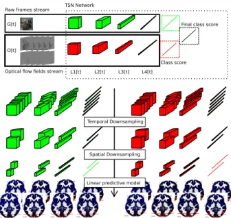
G[t]
O[t]
Final class score Raw frames stream
Optical flow fields stream TSN Network
L1[t] L2[t] L3[t] L4[t] Class score
Temporal DownsamplingTemporal Downsampling
Temporal DownsamplingSpatial Downsampling
Temporal DownsamplingLinear predictive model
Figure 1: Feature extraction and regression scheme: at each time frame we compute and extract the activities of four layers
L1, · · · , L4of the temporal segment network on a single frame
and on a stack of 5 consecutive optical flow fields. The ex-tracted activities are spatially and temporally down-sampled and then used to predict brain activity of subjects exposed to the video stimuli.
0.1. This procedure leads to different parameter values
de-pending on the chosen layer activities.
Figure 1 gives an overview of the pipeline used to extract and process deep video features to estimate the brain activity of subjects.
Results
The extracted deep network features lead to different pre-diction performance depending on the down-sampling proce-dure, the stream used and the localization of target voxels.
An efficient spatial compression scheme
We show that preserving the channel structure of the network during spatial compression procedure is key for developing an efficient compression scheme.
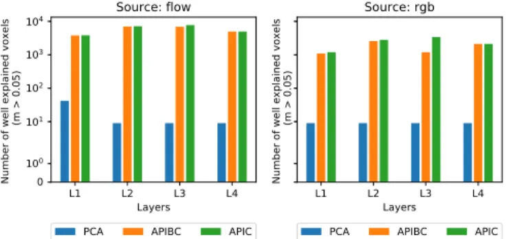
We compare three spatial compression schemes for net-work activities: (1) Standard principal component analysis
(PCA) with2000components; the transformation is learned
on training sessions before it is applied to all sessions. (2) Av-erage pooling inside channels (APIC) which computes local means of activities located in the same channel. (3) Average pooling inside and between convolution layers (APBIC) which is used to get the same number of output features for all layers while minimizing the number of convolutions between chan-nels. It allows us to check that the performance of the predic-tive algorithm is not merely driven by the number of features.
down-L1 L2 L3 L4 Layers 0 100 101 102 103 104
Number of well explained voxels
(m > 0.05)
Source: flow
PCA APIBC APIC
L1 L2 L3 L4 Layers
Number of well explained voxels
(m > 0.05)
Source: rgb
PCA APIBC APIC
Figure 2: Comparison of the different neural network com-pression streams. The APIC approach slightly outperforms APIBC, and both strongly outperform PCA. When using APIC or APIBC we predict correctly up to 850 times more voxels than when using PCA.
sampling and brain activity prediction is not changed while the spatial compression scheme varies. The benchmark is per-formed using a leave-one-out cross-validation procedure with two splits in three subjects.
Figure 2 shows that both approaches preserving channel organization structure outperform PCA by a large margin.
These results suggest that data stored in the same channel are similar and that mixing data between channels tends to destroy valuable information. In our pipeline, we average only inside same channels (APIC) because it yields the best per-formance. Choosing APBIC would be trading performance for computation speed since its high compression rate enables a much faster training of the prediction algorithm.
Data based parcellation of the brain using deep video representation
Depending on the considered region of the brain, the best fitting representation varies. We show that the compressed activities of different layers show contrasts between low-level (retinotopic) versus high-level (object-responsive) areas, but also between foveal and peripheral areas.
The difference between the prediction score from high level layer activity and low level layer activity of both streams (L4f low− L2f lowandLrgb4 − Lrgb2 ) yields a clear contrast between occipital (low-level) and lateral (high-level) areas (see Fig 3). This highlights a gradient of complexity in neural representa-tion along the ventral stream which was also found in (G ¨uc¸l ¨u & van Gerven, 2015).
The difference between predictions score from low-level layers activity of flow fields stream and high level layers activity
of raw frames stream (L1f low− Lrgb4 ) yields a contrast that does
not match boundaries between visual areas; instead, it does coincide with the retinotopic map displaying preferred eccen-tricity (see Figure 4). Intuitively this means that regions where brain activity is better predicted from the highest layer of opti-cal flow fields than from the lowest layer of raw frames stream are involved in peripheric vision whereas regions where ac-tivity is better predicted from the lowest layer of raw frames
Figure 3: High level and low level areas contrasts: Difference between predictions score from high level layer activity and
low level activity of the raw frames streamLrgb4 −Lrgb2 (top) and
flow fields streamL4f low− L2f low (bottom). The results show
a clear contrast between occipital areas better predicted by lower level layers (blue) and lateral areas better predicted from highest level layers (red), illustrating a gradient of complexity across areas. x=-6 L R z=0 -6 -3 0 3 6 L R y=-94 L1, flow - L4, rgb x=-6 L R z=0 -3.1 -1.6 0 1.6 3.1 L R y=-94 eccentricity
Figure 4: The difference between predictions score from low-level layers activity of flow fields and high-low-level layers activity
of raw frames streamL1f low− Lrgb4 (top) resembles the
pre-ferred eccentricity map of the same subject (bottom). Areas that are better predicted from low level flow fields streams are mostly involved in peripheric vision whereas areas better pre-dicted from high level raw frames stream are mainly foveal.
stream than from the highest layer of optical flow fields are mainly foveal.
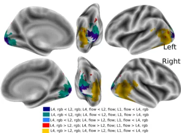
We use the contrasts between high level layers and low level layers, and the eccentricity related contrast to construct a parcellation of the brain based on these contrasts (see Fig-ure 5). From the 8 possible resulting profiles, three major clus-ters stand out allowing us to successfully depict a clustering of the voxels using contrasts from deep representation of the stimuli.
Discussion
Reproducing the results of (G ¨uc¸l ¨u & van Gerven, 2015) we have shown that lateral areas are best predicted by the last layers of both streams whereas occipital areas are best pre-dicted by first layers of both streams. We have also shown that foveal areas are best predicted by last layers of the raw
Figure 5: Parcellation summarizing artificial-biological corre-spondences: The set of active voxels were split into sub-groups according to their differential response to three
con-trasts: L2f low− L4f low, L2rgb− L4rgb, and L1f low− L4rgb.
From the 8 possible resulting profiles, 3 major clusters stand
out: deep blue,L2f low> L4f low,L2rgb> L4rgb, andL1f low<
L4rgb; it corresponds to a voxel set in primary visual areas that
has low eccentricity (foveal regions); green,L2f low> L4f low,
L2rgb> L4rgb, andL1f low> L4rgb, it corresponds to the same visual areas, but for voxels with higher eccentricity
(periph-eric voxels); yellow , L2f low < L4f low, L2rgb < L4rgb, and
L1f low< L4rgb, it corresponds to lateral and lateral visual ar-eas that encode more abstract representations of the objects.
frames stream and that peripheric areas are best predicted by the first layers of the flow fields stream. We have introduced a compression procedure for video representation that does not alter too much the channel structure of the network, yielding tremendous gains in performance compared to PCA.
The linear prediction from deep video features yields pre-dictions scores that are far better than chance. However the TVL1 algorithm (Zach, Pock, & Bischof, 2007) used in the TSN network does not produce high quality flow fields. Using more recent algorithms to compute optical flow such as Flownet 2 (Ilg et al., 2017), our performance could be further improved. The TSN Network would have to be retrained though.
In contrast to (G ¨uc¸l ¨u & van Gerven, 2017), the data used to train the network are not the same as the data presented to the subjects. We rely in fact on transfer between computer vision datasets and the visual content used for visual stimu-lation. This transfer is imperfect: the Berkeley video dataset contains videos of landscapes and animated pictures that are not present in the Kinetic dataset, which introduces some noise.
In conclusion, our study provides key insights that areas have a role linked to their retinotopic representation when per-forming action recognition. Future studies should focus on finessing this result by using a network tuned for other tasks.
Acknowledgments
This project has received funding from the European Union’s Horizon 2020 Research and Innovation Programme under Grant Agreement No. 720270 (HBP SGA1).
References
Eickenberg, M., Gramfort, A., Varoquaux, G., & Thirion, B. (2017). Seeing it all: Convolutional network layers map the function of the human visual system. NeuroImage, 152, 184–194.
G ¨uc¸l ¨u, U., & van Gerven, M. A. (2015). Deep neural networks reveal a gradient in the complexity of neural representations across the ventral stream. Journal of Neuroscience, 35(27), 10005–10014.
G ¨uc¸l ¨u, U., & van Gerven, M. A. (2017). Increasingly complex representations of natural movies across the dorsal stream are shared between subjects. NeuroImage, 145, 329–336. Ilg, E., Mayer, N., Saikia, T., Keuper, M., Dosovitskiy, A., &
Brox, T. (2017). Flownet 2.0: Evolution of optical flow esti-mation with deep networks. In Ieee conference on computer vision and pattern recognition (cvpr) (Vol. 2).
Kay, W., Carreira, J., Simonyan, K., Zhang, B., Hillier, C., Vi-jayanarasimhan, S., . . . others (2017). The kinetics human action video dataset. arXiv preprint arXiv:1705.06950. Lin, M., Chen, Q., & Yan, S. (2013). Network in network. arXiv
preprint arXiv:1312.4400.
Nishimoto, S., Vu, A., Naselaris, T., Benjamini, Y., Yu, B., & Gallant, J. L. (2011). Reconstructing visual experiences from brain activity evoked by natural movies. Current Biol-ogy , 21(19), 1641–1646.
Pinho, A., Amadon, A., Ruest, T., Fabre, M., Dohma-tob, I., E.and Denghien, Ginisty, C., . . . Thirion, B.
(2018). Individual brain charting. Retrieved 2018, from
https://project.inria.fr/IBC/
Poline, J.-B., & Brett, M. (2012, Aug). The general linear model and fmri: does love last forever? Neuroimage, 62(2), 871–880.
Simonyan, K., & Zisserman, A. (2014). Two-stream convolu-tional networks for action recognition in videos. In Advances in neural information processing systems (pp. 568–576). Szegedy, C., Vanhoucke, V., Ioffe, S., Shlens, J., & Wojna, Z.
(2016). Rethinking the inception architecture for computer vision. In Proceedings of the ieee conference on computer vision and pattern recognition (pp. 2818–2826).
Wang, L., Xiong, Y., Wang, Z., Qiao, Y., Lin, D., Tang, X., & Van Gool, L. (2016). Temporal segment networks: Towards good practices for deep action recognition. In European conference on computer vision (pp. 20–36).
Zach, C., Pock, T., & Bischof, H. (2007). A duality based approach for realtime tv-l 1 optical flow. In Joint pattern recognition symposium (pp. 214–223).