HAL Id: tel-01809518
https://tel.archives-ouvertes.fr/tel-01809518
Submitted on 6 Jun 2018HAL is a multi-disciplinary open access archive for the deposit and dissemination of sci-entific research documents, whether they are pub-lished or not. The documents may come from teaching and research institutions in France or abroad, or from public or private research centers.
L’archive ouverte pluridisciplinaire HAL, est destinée au dépôt et à la diffusion de documents scientifiques de niveau recherche, publiés ou non, émanant des établissements d’enseignement et de recherche français ou étrangers, des laboratoires publics ou privés.
data problems
Julio Toss
To cite this version:
Julio Toss. Parallel algorithms and data structures for interactive data problems. Distributed, Parallel, and Cluster Computing [cs.DC]. Université Grenoble Alpes; Universidade Federal do Rio Grande do Sul (Porto Alegre, Brésil), 2017. English. �NNT : 2017GREAM056�. �tel-01809518�
Pour obtenir le grade de
DOCTEUR DE LA COMMUNAUTE UNIVERSITE
GRENOBLE ALPES
préparée dans le cadre d’une cotutelle entre la
Communauté Université Grenoble Alpes
et
l’Universidade Federal do Rio Grande do Sul
Spécialité : Mathématiques, sciences et technologies de l’information, informatique
Arrêté ministériel : 25 mai 2016
Présentée par
Julio TOSS
Thèse dirigée par Bruno RAFFIN et João L. Dhil COMBA préparée au sein des Laboratoires LIG, INRIA et Inf UFRGS dans les Écoles Doctorales MSTII (UGA) et PPGC (UFRGS)
Algorithmes et Structures de
Données Parallèles pour
Applications Interactives
Thèse soutenue publiquement le 26 Octobre 2017,
devant le jury composé de : M. Bruno, RAFFIN
Directeur de Recherche, Université Grenoble Alpes, Directeur de thèse
M. João L. Dhil, COMBA
Maître de Conférences, Universidade Federal do Rio Grande do Sul, Directeur de thèse
M. Claudio, ESPERANÇA
Professeur, Universidade Federal do Rio de Janerio, Rapporteur
Mme. Carla Dal Sasso, FREITAS
Professeur, Universidade Federal do Rio Grande do Sul, Présidente
M. Luis Gustavo, NONATO
Professeur, Universidade de São Paulo, Rapporteur
M. Lucas M., Schnorr
Maître de Conférences, Universidade Federal do Rio Grande do Sul, Examinateur
PROGRAMA DE PÓS-GRADUAÇÃO EM COMPUTAÇÃO
JULIO TOSS
Parallel Algorithms and Data Structures for
Interactive Applications
Thesis prepared in a co-tutelle aggreement and presented in partial fulfillment
of the requirements for the degree of Doctor of Computer Science
Advisor (UFRGS):
Prof. Dr. João Luiz Dhil Comba Co-tutelle advisor (UGA):
Prof. Dr. Bruno Raffin
Porto Alegre August 2017
Toss, Julio
Parallel Algorithms and Data Structures for Interactive Appli-cations / Julio Toss. – Porto Alegre: PPGC da UFRGS, 2017.
83f.: il.
Thesis (Ph.D.) – Universidade Federal do Rio Grande do Sul. Programa de Pós-Graduação em Computação, Porto Alegre, BR– RS, 2017. Advisor: João Luiz Dhil Comba; Coadvisor: Bruno Raffin.
I. Dhil Comba, João Luiz. II. Raffin, Bruno. III. Título.
UNIVERSIDADE FEDERAL DO RIO GRANDE DO SUL Reitor: Prof. Rui Vicente Oppermann
Vice-Reitora: Profa. Jane Fraga Tutikian
Pró-Reitor de Pós-Graduação: Prof. Celso Giannetti Loureiro Chaves Diretora do Instituto de Informática: Profa. Carla Maria Dal Sasso Freitas
Coordenador do PPGC: Prof. João Luiz Dihl Comba
The quest for performance has been a constant through the history of computing systems. It has been more than a decade now since the sequential processing model had shown its first signs of exhaustion to keep performance improvements. Walls to the sequential com-putation pushed a paradigm shift and established the parallel processing as the standard in modern computing systems. With the widespread adoption of parallel computers, many algorithms and applications have been ported to fit these new architectures. However, in unconventional applications, with interactivity and real-time requirements, achieving efficient parallelizations is still a major challenge.
Real-time performance requirement shows up, for instance, in user-interactive simulations where the system must be able to react to the user’s input within a computation time-step of the simulation loop. The same kind of constraint appears in streaming data monitoring applications. For instance, when an external source of data, such as traffic sensors or social media posts, provides a continuous flow of information to be consumed by an on-line analysis system. The consumer system has to keep a controlled memory budget and deliver a fast processed information about the stream.
Common optimizations relying on pre-computed models or static index of data are not possible in these highly dynamic scenarios. The dynamic nature of the data brings up several performance issues originated from the problem decomposition for parallel pro-cessing and from the data locality maintenance for efficient cache utilization.
In this thesis we address data-dependent problems on two different applications: one on physically based simulations and another on streaming data analysis. To deal with the simulation problem, we present a parallel GPU algorithm for computing multiple shortest paths and Voronoi diagrams on a grid-like graph. Our contribution to the streaming data analysis problem is a parallelizable data structure, based on packed memory arrays, for indexing dynamic geo-located data while keeping good memory locality.
Keywords: Parallel processing. data locality. stream processing. real-time processing. physically based simulation.
RESUMO
A busca por desempenho tem sido uma constante na história dos sistemas computacio-nais. Ha mais de uma década, o modelo de processamento sequencial já mostrava seus primeiro sinais de exaustão pare suprir a crescente exigência por performance. Houve-ram "barreiras"para a computação sequencial que levaHouve-ram a uma mudança de paradigma e estabeleceram o processamento paralelo como padrão nos sistemas computacionais mo-dernos. Com a adoção generalizada de computadores paralelos, novos algoritmos foram desenvolvidos e aplicações reprojetadas para se adequar às características dessas novas arquiteturas. No entanto, em aplicações menos convencionais, com características de in-teratividade e tempo real, alcançar paralelizações eficientes ainda representa um grande desafio.
O requisito por desempenho de tempo real apresenta-se, por exemplo, em simulações in-terativas onde o sistema deve ser capaz de reagir às entradas do usuário dentro do tempo de uma iteração da simulação. O mesmo tipo de exigência aparece em aplicações de monitoramento de fluxos contínuos de dados (streams). Por exemplo, quando dados pro-venientes de sensores de tráfego ou postagens em redes sociais são produzidos em fluxo contínuo, o sistema de análise on-line deve ser capaz de processar essas informações em tempo real e ao mesmo tempo manter um consumo de memória controlada.
A natureza dinâmica desses dados traz diversos problemas de performance, tais como a decomposição do problema para processamento em paralelo e a manutenção da localidade de dados para uma utilização eficiente da memória cache. As estratégias de otimização tradicionais, que dependem de modelos pré-computados ou de índices estáticos sobre os dados, não atendem às exigências de performance necessárias nesses cenários.
Nesta tese, abordamos os problemas dependentes de dados em dois contextos diferen-tes: um na área de simulações baseada em física e outro em análise de dados em fluxo contínuo. Para o problema de simulação, apresentamos um algoritmo paralelo, em GPU, para computar múltiplos caminhos mínimos e diagramas de Voronoi em um grafo com topologia de grade. Para o problema de análise de fluxos de dados, apresentamos uma estrutura de dados paralelizável, baseada em Packed Memory Arrays, para indexar dados dinâmicos geo-localizados ao passo que mantém uma boa localidade de memória.
Palavras-chave: algoritmos paralelos, localidade de dados, processamento de fluxo de dados, processamento em tempo real, simulação baseada em física.
RÉSUMÉ
La quête de performance a été une constante à travers l’histoire des systèmes informa-tiques. Il y a plus d’une décennie maintenant, le modèle de traitement séquentiel montrait ses premiers signes d’épuisement pour satisfaire les exigences de performance. Les bar-rières du calcul séquentiel ont poussé à un changement de paradigme et ont établi le traitement parallèle comme standard dans les systèmes informatiques modernes. Avec l’adoption généralisée d’ordinateurs parallèles, de nombreux algorithmes et applications ont été développés pour s’adapter à ces nouvelles architectures. Cependant, dans des ap-plications non conventionnelles, avec des exigences d’interactivité et de temps réel, la parallélisation efficace est encore un défi majeur.
L’exigence de performance en temps réel apparaît, par exemple, dans les simulations in-teractives où le système doit prendre en compte l’entrée de l’utilisateur dans une itération de calcul de la boucle de simulation. Le même type de contrainte apparaît dans les ap-plications d’analyse de données en continu. Par exemple, lorsque des donnes issues de capteurs de trafic ou de messages de réseaux sociaux sont produites en flux continu, le système d’analyse doit être capable de traiter ces données à la volée rapidement sur ce flux tout en conservant un budget de mémoire contrôlé.
La caractéristique dynamique des données soulève plusieurs problèmes de performance tel que la décomposition du problème pour le traitement en parallèle et la maintenance de la localité mémoire pour une utilisation efficace du cache. Les optimisations classiques qui reposent sur des modèles pré-calculés ou sur l’indexation statique des données ne conduisent pas aux performances souhaitées.
Dans cette thèse, nous abordons les problèmes dépendants de données sur deux applica-tions différentes : la première dans le domaine de la simulation physique interactive et la seconde sur l’analyse des données en continu. Pour le problème de simulation, nous pré-sentons un algorithme GPU parallèle pour calculer les multiples plus courts chemins et des diagrammes de Voronoi sur un graphe en forme de grille. Pour le problème d’analyse de données en continu, nous présentons une structure de données parallélisable, basée sur des Packed Memory Arrays, pour indexer des données dynamiques géo-référencées tout en conservant une bonne localité de mémoire.
Mots clés: algorithmes parallèles, localité de données, traitement de flux de données, traitement en temps réel, simulation physique.
Figure 2.1 Voronoi diagram in Euclidean space for a given set of seeds...21
Figure 2.2 Sample shape function with two DoFs ...22
Figure 2.3 Frame-based simulation of complex deformable objects ...23
Figure 2.4 JFA: Jumping Flood Algorithm, step-by-step. ...25
Figure 2.5 Voronoi computation: labels encoding ...28
Figure 2.6 Scatter updates: label propagation to neighbor vertices ...29
Figure 2.7 Evolution of the updates in the thread activity mask...31
Figure 2.8 Voronoi diagram comparison with different mateial maps...32
Figure 2.9 GPU speed-up with varing input sizes...34
Figure 2.10 Trace of active threads by iteration of the RelaxKernel ...34
Figure 2.11 Average GPU speed-up with varing number of Voronoi seeds ...35
Figure 2.12 Stream compression algorithm ...37
Figure 2.13 Coarse stream compression algorithm...38
Figure 2.14 2D plan view of the activity mask with stream compression ...38
Figure 2.15 Profiling of stream compression optimization...39
Figure 2.16 NNI query example...42
Figure 2.17 Comparison of Sibson and Distance-ratio interpolation methods ...43
Figure 2.18 Parallel Sibson Interpolation Analysis...46
Figure 3.1 Example of PMA structure and densities ...51
Figure 3.2 Z-curve ordering with Morton codes...53
Figure 3.3 Examples of linear quadtrees and codes of each cell. ...54
Figure 3.4 PMQ: data structure overview ...59
Figure 3.5 PMQ: user interface overview ...64
Figure 3.6 Performance comparison of spatial data management solutions...69
Figure 3.7 PMQ insertion performance using Explicit indexing ...71
Figure 3.8 PMQ Insertion peformance in steady phase ...74
Figure 3.9 Performance comparison for range queries operations ...76
Figure 3.10 Performance comparison of Top-K queries...77
Figure 3.11 User interface demonstration: dynamic heatmap updates ...78
Figure 3.12 User interface demonstration: zooming and range selections ...79
Table 2.1 Summary of the performance benchmarks...33
Table 2.2 Computation time for parallel NNI queries...45
Table 3.1 PMQ insertion performance using Implicit indexing...71
Table 3.2 PMQ insertion time with varying time horizon...73
2.1 Shortest path computation: relaxation algorithm...27
2.2 Parallel Voronoi computation in CUDA (host code). ...30
2.3 CUDA kernel for the relaxation algorithm ...30
2.4 CUDA kernel for update and terminus verification ...30
1 INTRODUCTION...11
1.1 Outline...13
1.2 General Context And Motivations ...13
1.2.1 Walls to Sequential Computation...14
1.2.2 Big Data and Exascale Computing ...15
1.2.3 In-memory Big Data Processing...15
1.2.4 A Use Case Problem: Interactive Exploration of Geo-Located Data Streams. ...16
2 A PROBLEM ON PHYSICALLY BASED SIMULATIONS ...18
2.1 Context...18
2.2 Background ...20
2.2.1 Sofa - Simulation Framework ...20
2.2.2 Voronoi Diagrams ...20
2.2.3 Shape Functions in Numerical Simulation ...21
2.2.4 Material-Aware Shape Functions...23
2.3 Related Work...24
2.3.1 Parallel Voronoi Computations ...24
2.3.2 The Shortest Path Computation ...26
2.3.3 Existing Implementations of SSSP Algorithms...27
2.4 Parallel Graph Voronoi on GPU...27
2.4.1 Data Structure ...28
2.4.2 Parallel Algorithm...29
2.4.3 Experimental Evaluation...31
2.4.4 Results and Discussion ...32
2.4.5 Optimization with Stream Compression...36
2.4.6 Stream Compression Evaluation...37
2.4.7 Conclusion ...40
2.5 Parallel Voronoi-based Interpolations ...40
2.5.1 The Natural Neighbor Interpolation Method ...41
2.5.2 Voronoi Based Interpolation Methods ...41
2.5.3 Parallel NNI Algorithm...43
2.5.4 Performance Evaluation...45
2.5.5 Conclusions...46
3 A PROBLEM ON STREAMING DATA VISUALIZATION...48
3.1 Context...48
3.2 Background ...49
3.2.1 The Packed Memory Array (PMA) ...49
3.2.2 Z-curve...53
3.2.3 Linear Quadtrees...53
3.3 Related Work...54
3.3.1 Adaptive Sorting Algorithms ...55
3.3.2 Tree-Based Indexes...56
3.3.3 Cache-Oblivious Data Structures...56
3.3.4 Visual Analytics Data Structures ...57
3.4 The Packed-Memory Quadtree ...58
3.4.1 Overview...58
3.4.2 Implicit PMQ ...60
3.5.2 Range Queries...65
3.5.3 Top-K Queries...65
3.6 Implementation Details ...66
3.7 Performance Evaluation...67
3.7.1 Experimental protocol...68
3.7.2 Standard Database Solutions...68
3.7.3 PMQ Insertions ...70
3.7.4 Temporal Deletions...72
3.7.5 Range Queries...75
3.7.6 Top-K Performance...76
3.8 Closing Remarks on Performance...77
3.9 Use Cases of Interactive Exploration ...79
3.10 Conclusion ...81
4 FINAL REMARKS...82
1 INTRODUCTION
Since the invention of early computers, we have seen an impressive growth in the amount of applications and problems that could be solved by these machines. The role of computers have nowadays by far surpassed the applications thought by their inven-tors. A long road has been traveled, from the first calculation machines up to the modern supercomputers. Practical limits of what we can do with computers are still unknown. For every technology improvement made to the computing systems, new possibilities and challenges arise pushing the frontier of what can be done on these pieces of silicon. At the same time, scientists have created a kind of "chicken-egg" problem. For every new improvement made to current computing systems, larger problems and more demanding applications require the development of a new generation of computers. The quest for performance has been a constant through the computing history.
Amongst the fascinating possibilities, computers can simulate our world, capture information from it, process the data and output it back to the world in a glimpse of eyes. For a large class of applications, performance is closely related to the reactivity of the sys-tem, the ability to process information within a negligible time. Real-time processing for example happens in interactive simulation systems where the user can interact with a vir-tual model of the world without experiencing unrealistic delays. For instance, such kind of systems is common in medical simulation applications. The realism and complexity of the model to simulate is limited by the real-time processing power that the computing system is able to deliver.
Not only user-interactive systems require real-time processing. In big-data sys-tems, for instance, sensors from road networks or even social media on the web generate massive amounts of data every second. On-line data processing systems must be able to process the continuous stream of data to produce valuable information in real-time. In such cases, the maximum affordable computing performance limits the amount of infor-mation that can be digested on-the-fly.
Until recently, solutions to the performance requirements of these problems could rely on the sequential processing paradigm backed by a constant improvement on the sequential hardware architectures. This model of computing has now reached a point of exhaustion and is not able anymore to continue delivering the same growth in processing speed. Pushed by physics limitations, the computing paradigm made a shift to the parallel processing model. Nowadays, and until quantum computers become viable, any hope
for performance to keep the pace with the continuous increase of problems scale passes through the parallel computing paradigm.
Parallel processing capabilities are nowadays widespread and available in every computing device whatever its scale. Current operating systems already do a good job in scheduling different sequential applications to run concurrently on multicore processors. However the OS alone can’t provide individual applications. Application performance de-pend on how well the problem can be decomposed into indede-pendent tasks to benefit from parallel architectures. Generally, effective parallelization depends on two main aspects: Computation decomposition: how the amount of computation can be evenly distributed
among all the processing cores;
Memory access and locality: How to keep data close to the cores to reduce access la-tency, and how to maintain data locality during an interactive computation.
Some applications are trivially parallelizable, like on image processing, where fil-ters and transformations can be applied independently on each pixel in a data parallel style, also known as SIMD (Single Instruction Multiple Data). These problems are char-acterized by very limited data-dependency and by a balanced amount of computation of each piece of data, which make it simple to split and schedule for parallel execution. The computation to be executed and corresponding data are known since the beginning of the execution, allowing to optimize the data partitioning and scheduling on processors.
Unfortunately for the majority of applications, data partitioning and computation parallelization are not straightforward. In the case of interactive computation, like user-interactive physically based simulations or on-line streaming processing, data and com-putation are subject to the interactions of an external agent hard to predict. The chal-lenges presented on these domains require special data-structures and algorithms capable of adapting to the dynamic nature of the problems while still keeping good properties of memory locality and computational load balance.
In this research we tackle the challenges of parallelizing and keeping data locality in unconventional problems like interactive simulation and streaming data processing. Each problem has its particular characteristics but share a similar performance issue that has its roots on how to deal with data dependent computations dynamically. We deal with the performance problem of these two applications. To address it we propose two techniques, one targeting graphics parallel processors (GPUs) and another focusing in a dynamic data organization structure to maintain locality of references.
1.1 Outline
The core of this document is organized in chapters according to the contributions proposed:
• The first problem is related to physically based simulations: it involves a user-interactive system that changes the state of the data in a virtual model. Challenges on how to update data to keep the real-time execution of the simulation are ad-dressed by parallelizing the underlying data structures on the GPU. We present this problem and the associated contributions inChapter 2.
• The second one is on Big and Fast data processing: the real-time requirement in this case comes from the need of a data exploration system to keep the pace with a continuous real-time data stream. We propose a data-structure that stores the incoming information and is able to keep a good memory organization favoring data locality and speed-up queries on the data. The contributions are presented in
Chapter 3.
Additionally, before diving into the specific contribution topics, we provide further context that motivates our work on Section 1.2. Finally, the last chapter provides final remarks and perspectives for possible continuations of this work (Chapter 4).
1.2 General Context And Motivations
In this work we face problems of how to enhance the computation of data depen-dent problems. In the context of physically based simulations, we need to compute values based on neighborhood data. As we will see later inSection 2.3.3, the arithmetic opera-tions executed over them are simple and represent a much lower cost than accessing the data itself. Keeping data locality during the simulation is paramount.
One main characteristic of this problem is that with the right underlying data-structure we are able to expose the data parallelism underneath it. This leads us to propose efficient solutions based on the SIMT (Single Instruction Multiple Threads) paradigm of modern massively parallel architectures (GPUs). However optimizing load balance and occupation of these data-dependent programs still represents a major challenge. Effec-tively placing data in memory to speed-up locality access is a major concern to keep all the processors busy.
volume of data to process can change during execution and the pre-computed data de-pendency relations can be modified in unpredictable ways. Exploration of large datasets requires structure and organization of data to reduce memory access latency. Maintain-ing this organization when the dataset is dynamic and when the system has to respect real-time constraints is a challenging task. We refer to this problems as dynamic-data problems.
In the next sections we discuss the more fundamental problem of keeping the computational efficiency on dynamic-data problems. To understand the role that memory plays in computation and how historically computers turned into the parallel processing paradigm, we start with a brief review of how memory and computation capacities evolved over the past years and what are the boundaries they are facing. Finally we also present the current perspectives towards the era of exascale computing and big data problems that motivates our contribution on the development of new dynamic data structures for parallel machines.
1.2.1 Walls to Sequential Computation
The evolution from the sequential programming paradigm to the current parallel paradigm happened relatively recently in the past two decades (MCCOOL et al., 2012). The idea of parallel computation however is much older that this. There were factors that pushed a shift in the computing paradigm that are commonly know as the "three walls to sequential computation":
The Power wall refers to unacceptable increases in power consumption of the chip with the increase of processor clock rates. The maximum frequency at which a processor can operate has reached a limit and is now generally around 3Ghz. With the Moore’s law still holding true, the industry kept increasing the amount of transistors per unit area, which led to the design of multicore chips.
The Instruction-level parallelism (ILP) wall refers to a set of parallel techniques used at chip level that for some years allowed to speed-up sequential programs. Tech-niques like instruction pipelining, superescalar execution, out-of-order execution, register renaming, branch prediction, and speculative execution have fulfilled to a very large extent their potential.
The Memory wall is the consequence of several years of improvements in CPU process-ing speed that were not followed at the same rate by improvements in the memory speed. The memory and communication problems are related to two "speeds": la-tency and bandwidth . Latency is the time spent for starting a transaction. Once the transfer has started the bandwidth is the rate at which data is delivered at the destination. The use of larger caches allowed to temporarily cope with these prob-lems, however, latency is difficult to decrease due to fundamental physical limits such as the speed-of-light. On sequential processing streams the latency for a mem-ory access could not be hidden anymore causing the processor to stall waiting for data. Bandwidth on the other hand is easier to improve by increasing the number of lanes and sending big chunks of data at a time. This favored parallel executions for example in the SIMD computation paradigm.
1.2.2 Big Data and Exascale Computing
In the scientific and engineering community, exascale computing refers to com-puting systems able to process 1018
operations per second. To achieve this goal, industry and scientific community still have several challenges to tackle (REED; DONGARRA,
2015).
Big data is one of the main use cases that will benefit from exascale computing systems. Processing the enormous quantity of data generated today poses several chal-lenges in different fields. In the exascale regime, the energy cost to move a unit of data will exceed the cost of a floating-point operation (REED; DONGARRA,2015). Improve-ments on the hardware will continue to enhance memory features. New advanced memory technologies will provide large capacities and a high performance interconnect will pro-vide energy efficient, low-latency and high-bandwidth data exchange among hundreds of thousands of processors.
However, hardware improvements alone will fail to provide application speed-ups. At the software level there is still a need for locality aware algorithms to improve computation efficiency and reduce energy needs.
1.2.3 In-memory Big Data Processing
Big data has become widespread in industry with several systems being designed to address a wide range of problems (ZHANG et al.,2015). More recently, with the
cur-rent improvements in memory technologies like Non Volatile Memories (e.g. SSD) and larger capacities of DRAMs, traditional disk-base database systems have been shifting to a heavier use of in-memory storage and processing.
We may differentiate these data processing systems into "classes" according to the structureand dynamicity of data. Data-processing can be well structured like relational databases, semi-structured like graph processing, or completely unstructured as in texts. The dynamicity refers to the amount of insertion, deletion and update operations that are applied on the data. Such datasets can vary from a static set of records with regular updates with low insertion ratio, up to completely dynamic elements as in real-time streams of data. Each scenario requires different memory optimization techniques and often presents a trade-off between efficient indexing and querying of records. In this work we will focus on the problem of keeping an efficient update ratio on dynamic data while keeping good access performanceby favoring spatial locality.
1.2.4 A Use Case Problem: Interactive Exploration of Geo-Located Data Streams.
Several business applications rely on stream processing to get real-time knowl-edge about events currently happening and take fast decisions, such as in the stock mar-ket, sensor networks or in social networks. These systems often employ Complex Event Processing (CEP) to identify patterns of events in the stream and if needed triggers the appropriate alarm. The main characteristic of this stream processing is that historic data is usually not stored due to the high unbounded amount of data that a stream generates. This comes with the drawback that we must know in advance what kind of event we are expecting to setup a continuous query that will filter the incoming stream. Once an auto-matic alarm is triggered we have lost access to the previous historic raw data, which could have been useful for a more detailed analysis by a specialist.
For instance, a system that monitors microblogs streams such as twitter could de-tect natural disaster and point the location where humanitarian aids should be deployed with priority (SAKAKI et al., 2010). While storing full history of tweets would be un-practical and out of purpose, having a significant time window of past tweets stored about the area of interest would enable a more detailed analysis after a natural disaster alarm is triggered.
The real-time nature of such systems requires data to be resident in memory. This not only allows fast answer time of exploratory queries but also keeps a high rate of
in-sertions and index update capable of processing the incoming data stream. Furthermore, geo-spatial data must be indexed and stored in a way to provide fast access time. While several types of spatial-indices exist, it is important in real-time systems to avoid expen-sive updates and physical reorganization of data in memory.
2 A PROBLEM ON PHYSICALLY BASED SIMULATIONS
2.1 Context
Physically based simulations are widely used in several domains of applications. Digital animation, as used in films and games, rely on physical models to try to reproduce their behavior as realistically as possible to achieve the best visual effects. Physical mod-els, traditionally used in scientific computing and visualization domains, are also largely applied in the engineering industry. Here, the use of virtual models can help to anticipate problems in the project of a new product still in the earliest stages of conception, before going to production. For example, the automobile industry uses physically based simu-lations on virtual car models to perform crash tests, which permits reducing the number of expensive real crash tests. More recently, another growing field using this kind of sim-ulation is that of medical applications such as computer-assisted surgery. In this case, a physically based simulation can be used for planning and training surgical procedures reducing costs and avoiding complications during the real surgery.
On the other hand, the algorithms used in physically based simulations usually face a compromise between speed and accuracy (COURTECUISSE, 2011). This led us to analyze these application fields with different requirements. Computer games for ex-ample have a strong requirement for speed as it has to be done in real-time while accu-racy just needs to be approximated using a visually correct simulation. In contrast, virtual crash tests simulations, for example, require very accurate results but can be done offline. Surgery simulation is, perhaps, the most challenging field. Here, we have an equal in-terest for efficiency, to enable real-time, and accuracy to get valid simulation results that corresponds to the actual surgery on a human body.
Many methods have been proposed over the past decades for simulation of de-formable objects. A good survey on physically based dede-formable objects can be found in
(NEALEN et al.,2006). A common problem of these methods is the sampling size used.
Accuracy of simulation greatly depends on how many samples are used in the model. This is a major problem when we need to simulate deformations of a complex object composed of many different materials with various degrees of stiffness. Softer regions would require higher sampling than stiffer ones and would incur in higher computation costs.
In (FAURE et al., 2011) a new frame-based method is proposed to simulate
with sparse sampling combined with specific functions, called shape functions, to inter-polate deformations within the simulation nodes. Their major contribution was the use of a novel material-aware shape function that computes distances based on compliance. This approach allows to have fewer simulation nodes and still capture the most relevant defor-mation modes to achieve good realism. Computation of shape functions and placement of simulation nodes are done at initialization steps. After initialization, the simulation can efficiently run in real-time at interactive frame rates. However, if any topology mod-ification is applied to the object during the simulation, the initialization step needs to be recomputed. The overhead added by on-line modifications of the model is prohibitive for an interactive simulation. For example, if we simulate a cut of an organ during a virtual surgery, the whole distribution of simulation nodes and shape functions has to be recom-puted on-the-fly. Therefore, a major concern of this method is to speed up the computation of shape functions to allow real-time simulations.
At the same time, the hardware technology of modern computers has evolved con-siderably. Over the last decade, parallel computers have become ubiquitous and it is now usual to have multiple processors in the same computer. Massively parallel hardware such as Graphics Processing Units (GPU) are becoming commodity processors and can easily be found in general desktop computers. This clear trend of increasing the core count of modern processors has direct implications at the software and programming levels. Ef-ficiently programming applications for this kind of platform requires an extra amount of effort from programmers. Algorithms and data structures have to be carefully designed to harvest the benefits of parallelism. As a consequence, new parallel languages and pro-gramming tools have been developed to help on such tasks.
In this chapter we look into the method of sparse meshless simulation proposed by
Faure et al.(2011) and study a parallel approach to the costly initialization steps where
the shape functions are computed. Material-aware shape function computation involves computing a special kind of Voronoi diagram on a graph with grid topology. We will abstract the concepts from the physically based simulation domain and focus on the algo-rithms. As we will see, the underlying problem is strongly related to the Multiple-Source Shortest Path (MSSP) problem.
In the next sections we will present in more details how shape functions are com-puted and what kind of algorithms are used (Section 2.2). InSection 2.3we review the related works about parallel computation of Voronoi diagrams and shortest-paths.
2.2 Background
2.2.1 Sofa - Simulation Framework
The work described in this chapter is part of the real-time simulation framework called SOFA (2017). It results from a cooperation work with the IMAGINE research team1 from Inria-Alpes, one of the main contributors to the development of SOFA.
The Simulation Open Framework Architecture (SOFA, 2017) seeks to reduce complexity in interactive physically based simulations by providing a well-defined com-mon interface for physical algorithms. Its goal is to improve research collaborations, al-lowing to reuse and easily compare a variety of available methods. Although the primary target application of SOFA is medical simulation such as in virtual surgery, applications from different domains also rely on this framework. Examples include motion planning and control in robotics simulations (LARGILLIERE et al., 2015; RODRIGUEZ et al.,
2017), augmented reality in deformable objects (PAULUS et al., 2015) and virtual im-mersion environments (PETIT et al.,2009).
The current SOFA implementation targets execution on a single machine, with some extensions allowing parallel applications on multicore and GPUs, but not on clus-ters or supercompuclus-ters architectures. The use of parallelism in this framework is highly desirable as a way of enhancing the performance of its simulation algorithms. The con-tribution we bring to the SOFA project is a new parallel algorithm for Voronoi-shape functions computation.
2.2.2 Voronoi Diagrams
The Voronoi diagram is a data structure extensively studied in the context of com-putational geometry for many different applications, but most of the time on a contiguous Euclidean space (RONG et al., 2011) or computing its discrete approximation (HOFF
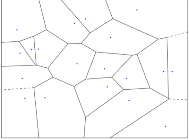
et al., 1999; RONG; TAN, 2006). Originally the Voronoi diagram (Figure 2.1) was
de-fined for a set of seed points P = {p1, p2, ..., pn} as the partitioning of the space into n
cells such that every seed pk is the closest one to any other point enclosed in the cell k,
according to a distance metric (usually Euclidean distance)(BERG et al.,2008).
Another particular type of Voronoi diagram is the Centroidal Voronoi Diagram, also known as Centroidal Voronoi Tessellation (CVT). In this case, the seeds must be the
Figure 2.1: Voronoi diagram in Euclidean space for a given set of seeds (blue dots).
centroids of their cells. The computation of a CVT is usually done using the Lloyd’s algorithm. In this iterative method, seeds are moved to the current center of each cell and the Voronoi diagram is recomputed at each iteration until convergence.
Although most works found on the literature study Voronoi diagrams on the Eu-clidean space, there are situations where a distance is defined using other metrics, such as the distance between vertices in a graph (ERWIG, 2000; HURTADO et al., 2004). In this context, the distance metric considered corresponds to the shortest path (also re-ferred as geodesic) between two vertices. This formulation of Voronoi diagrams arises, for instance, in the problem of facility location, where clients and suppliers lie in an inter-connection network. Computing these Voronoi diagrams basically consists in computing the shortest paths on a weighted graph.
The Parallel Dijkstra algorithm proposed byErwig(2000) is a variant to the Dijk-stra algorithm for computing the Voronoi diagram on directed weighted graphs. The term "Parallel" in this algorithm refers to the fact that the shortest-path trees, rooted at each Voronoi seed, grow rather simultaneously, although the algorithm is still sequential.
2.2.3 Shape Functions in Numerical Simulation
In computer graphics, the numerical simulation of continuous deformable objects is based on a set of independent control points called Degrees of Freedom (DoFs). For instance, in the popular Finite Element Method (FEM), the DoFs are the vertices of the mesh representing the discretized model.
In this work we deal with another particular class of methods for modeling de-formable objects know as meshless models. In particular, in the meshless frame-based models proposed byGilles et al.(2011), the simulation does not use any underlying
struc-Figure 2.2: Example of an object with two Degrees of Freedom (q0 and q1) and their
corresponding shape functions (W0 and W1). Displacement of a point u is the weighted
sum of sampled displacements at q0and q1.
q
0u
Shape function W0q
1u
Shape function W1 0.0 0.5 1.0ture like a mesh. In this case, the DoFs are unstructured control points called frames to which are associated shape functions. For each control point of the model there is a cor-responding shape function that defines a region of influence. The design of theses shape functions plays a central role in the simulation. It will determine how the displacements captured at different control points will be combined to result in the final deformation of the object.
Consider the following steps when simulating the deformation on an object sub-jected to some forces. The displacement of the object is sampled at the control points (DoFs). Each DoF and associated shape function define where and how other points in the object are influenced. This region of influence is commonly referred as the support of the shape function, i.e. the region of the object where the function is defined. The evaluation of the shape function at any point within the support results in a normalized weight that encodes the influence of the corresponding DoF at that point. In general, these weights decrease with the distance to the control point. For instance, inFigure 2.2
there are two control points in the object (red dots). The shape function of each one is defined everywhere within the object boundaries. Their normalized weights are shown by a heatmap and varies from 1, at each respective frame’s location, down to zero at the coordinates of the other frames. The displacement at any point u (green dot), parame-terized with coordinates x in the object, is therefore computed by a weighted sum of the displacements sampled at the DoFs (Equation 2.1).
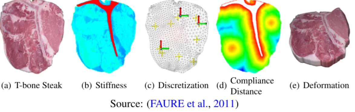
Figure 2.3: A frame-based method to simulate complex deformable solids composed with heterogeneous material properties.
(a) T-bone Steak (b) Stiffness (c) Discretization (d) Compliance
Distance (e) Deformation
Source: (FAURE et al.,2011)
Finally, it remains the problem of defining how weights should be computed for a given placement of control nodes. These weights describe how shape functions from dif-ferent DoFs are blended on the rest of the domain. In (FAURE et al.,2011), these weights are computed using a novel method based on Voronoi diagrams, called the Voronoi Shape Functions. We conceptually explain their method in the next section. A more detailed dis-cussion on shape functions is deferred toSection 2.5where we describe different schemes for interpolating node values using the Voronoi diagram generated from the simulation nodes.
2.2.4 Material-Aware Shape Functions
This section briefly introduces the frame-based simulation method presented in
(FAURE et al.,2011), which is the motivation problem of this chapter.
Shape functions are a fundamental part in the simulation of deformable solids. They are used to compute the displacement in the object within the simulation nodes. The displacement applied to simulation nodes is combined according to their shape functions (also called weights) and is interpolated inside the deformed object.
A material-aware shape function takes into account the material properties, such as stiffness, to compute the displacement. This is particularly interesting in objects com-posed with various types of materials, with different stiffness, as these regions will not deform in the same way or with the same intensity. For example, a steak composed of bones, fat and flesh will present different degrees of deformation in each material region (Figure 2.3).
The input data for this method is given as a 3D voxel map of material properties and a quantity of simulation nodes according to the expected execution time. The prob-lem consists in defining the placement of nodes and the shape function associated. A
major challenge here is to define a proper region of influence of each shape function. For example, consider the steak object fromFigure 2.3, a deformation applied to a node on the left side of the rigid bone should not be propagated to the other side.
To limit this kind of unrealistic behaviour, the authors create Voronoi partitions of the voxelized material property map. Similarly, the problem of placement of simulation nodes can be approached as the Centroidal Voronoi Diagram computation on a weighted graph. The distances used to compute the Voronoi diagrams are based on the values of compliance (inverse of stiffness) of each voxel. The compliance distance, as referred in their work, is the length (compliance) of the shortest (stiffest) path from one point to the other.
We highlight some specific features in this problem that differs from a general Voronoi computation. First of all, it should be noted that the Voronoi diagram here is not computed on the Euclidean space. This means that distances between any two points cannot be computed directly. Instead, we have a geodesic on a 3D discrete voxel map where each voxel knows the local distances (compliance distance computed from the material property map) in its 26-neighborhood. Each voxel is mapped to a vertex of the graph and is connected with the 26 vertices corresponding to the adjacent voxels in a 3D image 2. Finally, edges are weighted according to the compliance value of the pair of
adjacent voxels.
2.3 Related Work
2.3.1 Parallel Voronoi Computations
The parallelization of Voronoi diagram computations has been studied through several works in literature with a lot of different approaches. Early studies used graphics hardware to compute an approximation of these diagrams using the OpenGL graphics library, before the proposal of the CUDA or OpenCL architecture (HOFF et al., 1999). For most works found in the literature, a discrete approximation of the Voronoi diagram is sufficient to fulfill the precision requirements of its applications. Approximations can be either computed by the Euclidean distance on 2D pixel-maps and in 3D surfaces using the Euclidean distance between 3D-coordinates of sampled points over the surface (RONG et
al.,2011).
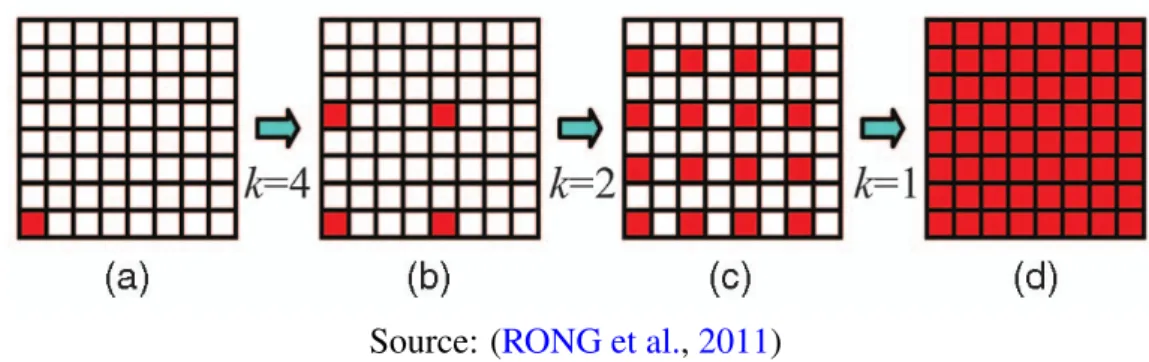
Figure 2.4: JFA: starts propagating the information from the seed (bottom left corner). At each step, the neighbours with coordinates offset k are reached and start propagating the data about the seed.
Source: (RONG et al.,2011)
The many parallel approaches vary in the way the information of proximity from the Voronoi centers is propagated to each pixel.
Rong and Tan(2006) propose jump flooding (JFA) as an algorithmic paradigm for
GPGPU and show its application on Voronoi diagram computation. In JFA, the seeds start propagating their coordinates to neighbour pixels according to a pattern that halves the offset at each step (Figure 2.4). Each pixel compares the new information received with the previous one and keep the coordinates of the closest seed. In this case, distances can easily be computed on the Euclidean plane.
Weber et al. (2008) introduce an interesting parallel algorithm called parallel
marching method (PMM)to compute distances on surfaces with application on Voronoi diagrams. This method is indeed an extension of the fast marching method, which is based on a priority-queue. However, this kind of data structure is difficult to be efficiently parallelized. Instead, their method replaces it by using a specific traversing order of the grid, called raster scan, and show an efficient parallelization algorithm.
Reem(2012) proposed a substantially different method from previous ones. It uses a combinatorial approach to compute the exact polygons that form each cell of the Voronoi diagram in parallel. This work, however, is mainly theoretical, focusing on formal proofs of correctness and complexity analysis while leaving aside the implementation issues and experimental results.
All of these works only consider distance computation on the Euclidean space. None of them were found to deal with Voronoi diagrams on graph space. In those contexts the shortest distance is always a straight line, hence these methods cannot be directly applied on graph problems. Nonetheless,Weber et al.(2008) show that PMM can also be used to compute distance on curved domains by repeating Niteriterations of raster scans,
2.3.2 The Shortest Path Computation
Clearly, the shortest-path problem is an essential building-block for Voronoi dia-gram computation on graphs. Efficiently finding shortest paths on graphs is a well known problem widely studied in the literature for a plethora of applications. Probably the best known sequential algorithm for Single-Source Shortest-Path (SSSP) was developed by Dijkstra. The original Dijkstra’s algorithm has O(V2
) complexity on the number of ver-tices, while the min-priority-queue based version shows O(E + V logV ) where E is the number of edges (CORMEN et al.,2009).
Naturally, the use of parallel processors to compute shortest paths has attracted a lot of attention from researchers. Early implementation of a parallel Dijkstra’s SSSP is reported in (CRAUSER et al.,1998). However, this is an inherently sequential algorithm with lots of synchronizations leaving no possibility for an efficient PRAM implementation
(HARISH et al., 2009). As an alternative,Kumar et al.(2011), worked on parallel SSSP
based on Bellman-Ford’s algorithm, which is less efficient than Dijkstra on sequential implementations but has a higher degree of parallelism.
Most of the parallel SSSP algorithms introduced in the literature have to deal with a trade-off between the amount of parallelism exposed and the extra work generated.
Madduri et al.(2006) proposes a parallel ∆−stepping method that shows a good
compro-mise between these two factors. They report an implementation exhibiting 30x speed-up on a CRAY MTA-2 shared memory architecture with 40 processors.
Implementations on Graphics Processors also showed to be a viable and relatively cheap solution for SSSP computation (HARISH et al., 2009; HARISH; NARAYANAN,
2007). On massively dense graphs, Kumar et al. (2011) use a modified Bellman-Ford algorithm on GPU and reports 10 to 12 times speedup over previous work for SSSP com-putation.
Edmonds et al.(2006) introduce the Parallel Boost Graph Library (Parallel BGL),
a library of graph algorithms for distributed-memory computation on large graphs. Their implementation of SSSP extends Dijkstra by allowing to remove several vertices at once from the top of the priority queue. This technique is used to expose more parallelism but introduces unnecessary computation of edges.
Regarding the graph topologies, the literature shows that, in general, the pro-posed methods scale better on random-topology graphs with regular vertex-degrees than on structured graphs (grid-like topology) or scale-free graphs (containing few vertices
with very high degree and a large majority with small degree) (EDMONDS et al., 2006;
HARISH et al.,2009;HARISH; NARAYANAN,2007).
2.3.3 Existing Implementations of SSSP Algorithms
Several GPU implementations have been proposed over the last years for differ-ent graph algorithms (HARISH et al., 2009). For the shortest path problem specifically, Dijkstra-based parallelizations are more frequently used (MADDURI et al.,2006;
HAR-ISH et al., 2009; ORTEGA-ARRANZ et al., 2013). Even so, there are also other
ap-proaches based on the Bellman-Ford algorithm, like on (KUMAR et al., 2011) targeting dense graphs on GPUs.
In general, Dijkstra based algorithms use a technique known as edge relaxation. In this technique, each vertex maintains a shortest-path estimate with distance v.d. The process of relaxation consists of trying to improve this estimate by going from vertex u to v through an edge of weight w(u, v) (Algorithm 2.1).
Algorithm 2.1 Shortest path computation: relaxation algorithm
1: procedure RELAX(u, v, w) 2: if v.d > u.d + w(u, v) then 3: v.d ← u.d + w(u, v) 4: end if
5: end procedure
When done in parallel, each vertex u is assigned to threads that may update v.d concurrently, thus creating a critical section. Consequently, lines2-4, ofAlgorithm 2.1, have to be protected in an atomic region. In modern CUDA devices this atomic region can be efficiently implemented by the single atomic instruction atomic_min(addr, val) .
atomic_min(addr, val) reads word old located at the address addr,
com-putes the minimum ofoldandval, and stores the result back to memory at the
same address. These three operations are performed in one atomic transaction (NVIDIA,2017).
2.4 Parallel Graph Voronoi on GPU
We present in this section our parallel algorithm for computing Voronoi diagrams on graphs. As mentioned previously, the Graph Voronoi can be seen as an extension of the shortest path problem. However, its parallelization poses additional problems of con-current access to shared variables. In the Voronoi diagram problem, each voxel has to
Figure 2.5: Encoding information of distance and Voronoi index in a single word. Values dand k can be changed to adjust precision.
Distance estimate Voronoi Index
32-bit word
d bits k bits
keep the distance estimate value to the seed and an extra variable for its Voronoi cell in-dex. These variables would then be updated serially in the relaxation procedure, which, if executed by two threads in parallel, could lead to any combination of results in these variables. On concurrent programming this is a classical case of race condition. The straightforward solution for this problem would be to enclose the whole critical section (Algorithm 2.1) within mutex locks. However, mutexes are expensive structures to imple-ment on GPUs. To deal with this problem, we choose to encode both variables, Voronoi index and distance estimate, in a single 32-bit word (Figure 2.5) that can then be atomi-cally updated in a single atomic_min() instruction. Our encoding can be adjusted to bal-ance distbal-ance precision and maximum number of Voronoi cells. In our implementation, we reserved 24 bits for the distance and 8 bits for the Voronoi region index.
2.4.1 Data Structure
Our data representation in memory substantially differs from the classical graph data structures. Instead of using adjacency matrices or lists for the shortest path compu-tation, like in (HARISH et al., 2009), we are dealing directly with 3D images of voxels. In order to use the graph nomenclature, we refer to voxels as nodes of a graph. Each node has in general 26 neighbors (except at the image boundaries). Information stored at each node contains its compliance value, Voronoi cell index, and distance to a Voronoi source. The weight of each edge is given by some generalized distance function, dist(Cv, Cu),
defined for every pair of voxels (v, u) as long as they are adjacent in the image. In this work specifically, we employ the compliance scaled distance function used by Faure et Al. (FAURE et al., 2011). In this case, the distance between two adjacent nodes is a function of the measure of compliance of the material at each node.
Figure 2.6: Scatter updates: each active thread propagates its current information about distance and Voronoi index to its neighbors.
2.4.2 Parallel Algorithm
Our algorithm uses five internal arrays, C0, C1, Vor, Mask and Mat, stored on the
GPU global memory. Each one has the same size of the input volume (Algorithm 2.2). The Mat matrix contains the discretized material map, and is used to computed the dis-tance between neighbor voxels. The cost arrays C0 and C1 are used to keep the
shortest-path estimates of each voxel. They are initialized with 0 at the seeds and ∞ (maximum unsigned integer value) everywhere else. The Voronoi diagram, stored on array Vor, is initially empty on every voxel, except for those corresponding to the seed’s coordinate that are initialized with a unique Voronoi cell index. Finally, the boolean array Mask is used as activity mask to mark which voxels have an updated cost estimate indicating that it will be relaxed on the next step.
We assign one thread to every voxel. The execution then follows a scatter approach (Figure 2.6) where each active thread, marked on Mask, will relax the cost estimate of its neighbors and set their correct Voronoi index. The algorithm is divided in two par-allel phases: relaxation and update. The host code (Algorithm 2.2) initializes the data structures and then iteratively calls the GPU kernels RELAXKERNEL (Algorithm 2.3),
add UPDATEKERNEL (Algorithm 2.4), until the termination condition is satisfied. The
distance function, at line5in RELAXKERNEL, computes the local distance between two
neighbor voxels based on their compliance values in the material map (FAURE et al.,
2011). At each iteration, C1 maintains the intermediate values computed during the
and the activity mask is updated. The duplication of these cost matrices is needed to avoid read-after-write hazards when writing to global memory.
Algorithm 2.2 Parallel Voronoi computation in CUDA (host code).
1: procedure VORONOI(Seeds,Vor,Mat) 2: for all v ∈ Mat do
3: C0[v] ← ∞; C1[v] ← ∞ 4: end for
5: for all s ∈ Seeds do 6: C0[s] ← 0; C1[s] ← 0 7: Mask[s] ← true
8: Vor[s] ← idx + +
9: end for 10: repeat
11: RELAXKERNEL(Mask,C0,C1,Mat) 12: TERM ← true
13: UPDATEKERNEL(Mask,C0,C1) 14: until TERM
15: end procedure
Algorithm 2.3 CUDA kernel for the relaxation algorithm: atomically updates the current shortest path estimates and the closest Voronoi seed.
1: procedure RELAXKERNEL 2: tid ← getV oxelIndex() 3: if Mask[tid] then
4: for all neighbors nid of tid do
5: dnew ← C0[tid] + localDist(tid, nid, M at)
6: AtomicMin((C1[nid]|Vor[nid]), (dnew|Vor[tid])) 7: end for
8: Mask[tid] ← false
9: end if 10: end procedure
Algorithm 2.4 CUDA update kernel: verifies the termination condition and updates the activity mask.
1: procedure UPDATEKERNEL 2: tid ← getT hreadIndex() 3: if C0[tid] > C1[tid] then 4: C0[tid] ← C1[tid] 5: Mask[tid] ← true
6: TERM ← false
7: end if 8: end procedure
Figure 2.7: At each iteration, the thread activity mask is updated. This process triggers propagation waves leaving from each Voronoi seed (red dots). As the distances are not linear some pixels will be recomputed causing the effect of "thicker waves" (b).
(a) Iteration 3 (b) Iteration 17 (c) Iteration 42
The propagation of distance and cell Id starts simultaneously at each seed and, for each iteration of lines11to13inAlgorithm 2.2, are expanded one step further away. Plot-ting the trace of thread activations at each step generates the wave-like pattern shown in the 2D plan ofFigure 2.7. The algorithm finishes when the Voronoi diagram computation reaches a fixed point, where no more voxel is updated.
2.4.3 Experimental Evaluation
Several benchmarks were performed to evaluate the performance of our algorithm. In the following sections we describe our test environment and input instances used for the experiments.
2.4.3.1 Test Environment
The platform used for the CPU benchmarks was an Intel CoreTM i7 CPU model
930 with 4 cores running at 2.89Ghz and 12 GB memory. Despite the multi-core archi-tecture, the CPU implementation is strictly sequential.
The results of our GPU algorithm were obtained on a NVIDIA GPU GTX480 with 1.5 GBytes of global memory and 15 Multiprocessors with 32 cores each, totaling 480 CUDA cores. The CPU codes were compiled with GCC 4.8 using -O2 optimization flags. The CUDA driver is version 6 while the run-time is version 5.5.
Figure 2.8: Comparison of Voronoi diagrams generated with the same set of seeds on two different material maps. Left: with an uniform stiffness. Right: with a stiffness gradient.
2.4.3.2 Input Instances
The input dataset differs on 3 different parameters: volume size, material map topology and number of Voronoi seeds. For the material map topologies we considered both synthetic and real-application data. The synthetic topologies represents a cube vol-ume with (a) an uniform constant stiffness and (b) a gradient stiffness varying uniformly from left to right (called Gradient). In these topologies, we variate the volume from 323
to 2563voxels, which are the common discretization sizes used for physically based
simula-tions in (FAURE et al.,2011). For each volume size, a placement of seeds was randomly generated and kept constant for each run of the benchmark. We note that, due to the compliance-scaled distance function employed, the same set of seeds actually generate very different Voronoi diagrams, depending on the topology of the material map used (seeFigure 2.8).
The real-application dataset is the discretized material map of the T-bone steak (Figure 2.3). The map of the steak has a volume of size 64x64x15 voxels and exhibits non-uniform stiffness distribution. The data of the steak is freely available for download with the SOFA framework (SOFA,2017;FAURE et al.,2012).
2.4.4 Results and Discussion
In this section we evaluate the implementation described in the previous sections. Performance of Voronoi computation is analyzed regarding 3 main parameters: volume size, topology of the material map and number seeds of the diagram. Following these
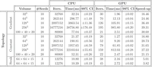
Table 2.1: Benchmark results with execution times and speed-up obtained with the base GPU algorithm.
CPU GPU
Volume #Seeds Iters. Time(ms) 99% CI Iters. Time(ms) 99% CI Speed-up
T o p o lo g y G ra d ie n t 32 3 10 32768 32.24 ±0.23 30 1.96 ±0.02 16.46 643 10 262144 296.77 ±1.48 70 12.13 ±0.04 24.46 1283 10 2097152 3863.54 ±11.36 126 105.91 ±0.15 36.48 2563 10 16777216 38756.80 ±176.48 195 985.80 ±0.20 39.31 100 × 40 × 20 20 80000 77.04 ±0.37 21 2.51 ±0.02 30.68 C o n st a n t 32 3 10 32768 21.37 ±0.19 20 1.27 ±0.01 16.80 643 10 262144 190.81 ±0.56 52 9.20 ±0.03 20.73 1283 10 2097152 1957.65 ±6.59 79 61.85 ±0.02 31.65 2563 10 16777216 22103.64 ±55.85 159 812.03 ±0.28 27.22 100 × 40 × 20 20 80000 52.31 ±0.26 22 2.47 ±0.01 21.15 S te a k 64 × 64 × 15 3 12276 10.80 ±0.10 38 2.16 ±0.03 5.01 64 × 64 × 15 10 12276 10.39 ±0.19 45 2.72 ±0.02 3.82
results we proposed an enhancement to the base algorithm which will be presented on
Section 2.4.5.
2.4.4.1 Base Algorithm Speed-up
We start by comparing our parallel algorithm with its sequential reference imple-mentation on CPU. For each input instance, we ran the benchmark 10 times, for the CPU and GPU algorithms, and computed the mean execution time. The obtained means and 99% confidence intervals are reported inTable 2.1.
Figure 2.9 presents the speed-ups obtained with GPU implementation over the sequential one on CPU. Each bar represents a different input instance where labels cube32310s, cube643
10s , cube1283
10s and cube2563
10s denote a cube with gradient topology with dimensions 32, 64, 128 and 256 respectively, each with 10 seeds. The plate 100x40x10 20sinput is a plate of stiffness gradient with 20 seeds. Both steak instances have a bounding volume of 64x64x15 voxels.
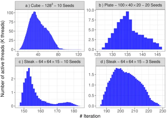
In this benchmark the speedup achieved varies from 3.8x for small volumes (Steak) up to almost 40x for bigger ones. These results show that our algorithm bene-fits from bigger input sizes, because they expose more parallelism. This observation is also confirmed by the trace of thread activity shown inFigure 2.10. Notice for instance the different scale on y-axis between facets (a) and (b) (Figure 2.10) showing a higher maximum of active parallel threads in the Cube volume of size 1283 than in the Plate
Figure 2.9: Speed-up for different input sizes. Gradient and constant topologies are presented for synthetic benchmarks only. Steak’s topology corresponds to the real data-set ofFigure 2.3. 0 10 20 30 40 Cube 32³ 10s Cube 64³ 10s Cube 128³ 10s Cube 256³ 10s Plate 100x40x20 20s Steak 64x64x15 3s Steak 64x64x15 10s Benchmark instances Speed-up CPU/GPU
Topology: Constant Gradient Steak
Figure 2.10: Trace of the number of active threads running in RELAXKERNEL at each
each iteration ofAlgorithm 2.2. (threads counted in thousands on the y axis)}
c ) Steak − 64 × 64 × 15 − 10 Seeds d ) Steak − 64 × 64 × 15 − 3 Seeds a ) Cube − 1283 − 10 Seeds b ) Plate − 100 × 40 × 20 − 20 Seeds
150 160 170 180 190 200 210 220 230 0 40 80 120 125 130 135 140 145 0.0 2.5 5.0 7.5 10.0 0.0 0.5 1.0 1.5 0 25 50 75 100 0 1 2 # Iteration Number of activ e threads (K threads)
Figure 2.11: Average speed-up when increasing the number of seeds of the Voronoi diagram. Standard deviations are shown on top of each bar.
0 20 40 60
1 2 4 8 16 32 64 128 256
Number of seeds of the Voronoi diagram
A
ver
age Speed−up CPU/GPU
2.4.4.2 Voronoi Seeds
On a second scenario, we investigated the impact of the number of seeds in the performance. For this benchmark we fixed the volume size at 1283
and used the same gradient topology to vary the number of seeds. For each number, we randomly generated 10 different seed placements.
The execution time was measured for each configuration of seeds and the speed-up was computed. Each reported value in the bar plot ofFigure 2.11is an average of the speed-ups over 10 different seed placements. The standard deviation plotted on top of each bar gives a notion of the variability of the speed-up according to the placement of seeds in the object. With more than 4 seeds, these results suggest that for larger amounts of seeds the speed-up generally increases. Indeed, having more Voronoi seeds has the effect of allowing more active threads right at the first iterations. Moreover, assuming a uniform distribution of seeds, the number of iterations of the algorithm tends to reduce as more Voronoi cells expand concurrently. Notice the different number of iterations (x-axis) shown onFigure 2.10, facets (c) and (d) (same volume with 10 and 3 seeds respectively). In real scenarios, more sophisticated algorithms are used to configure the place-ment of seeds. However, the rationale behind them is usually to keep a uniform
dis-tribution over the material map. Therefore, the random placement strategy used in this experiment remains a fair choice for our synthetic benchmarks.
2.4.5 Optimization with Stream Compression
The base implementation presented on the previous section already exhibits con-siderable speed-up over the sequential algorithm. The mapping from voxels on the volume to CUDA threads is done directly. This means that for a volume of dimensions 323
, there will be 323 threads, one for each voxel, deployed every iteration of the algorithm. This
direct mapping from pixels to threads is a common practice on GPU algorithms and bene-fits from their lightweight thread scheduling features. Nonetheless, as observed in picture
Figure 2.10andFigure 2.7, the number of threads that are actually updating values at each iteration is much smaller than the total size of the volume (i.e. the amount of threads de-ployed at each iteration).Figure 2.7shows how the computation propagates to neighbors in a wave-like form. The black front indicates, at each step, which threads are set to true in the activity mask at the beginning of the relaxation kernel (line3 in Algorithm 2.3). Over the execution of the algorithm, the number of active threads is much lower than the total grid size and varies considerably along time (Figure 2.10). This causes our thread blocks to be very inefficient as most of the threads will actually evaluate the conditional to false, without computing anything (line3,Algorithm 2.3) .
One might question if a finer control of the number of threads reflects in a better utilization of the GPU with consequent performance enhancements. To tackle this is-sue, we proposed a modification to our base algorithm that applies a technique known as stream compression(HOBEROCK et al.,2009;HARISH et al.,2009).
With stream compression, we perform an extra pass on the activity mask to count the number of voxels marked for update and to generate a new indirect mapping from thread Ids to voxel Ids. This way, the active threads are grouped in fewer and more com-pact blocks, thus reducing branch divergence and runtime overhead of scheduling idle threads. Stream compression is achieved by a Scan operation over the activity mask fol-lowed by a Scatter as shown inFigure 2.12. These operations can be easily implemented in CUDA using the Thrust template library (HOBEROCK; BELL, 2011). The result of the compression is an array mapping thread indices to voxel coordinates, that are used in the RELAXKERNELto retrieve the correct data (Algorithm 2.3line2).
super-Figure 2.12: Stream compression can be used to deploy only the exact amount of threads required to update the active voxels.
0 1 1 0 0 0 1 1 0 1 2 3 4 5 6 7 0 0 1 2 2 2 2 3 1 2 6 7 0 1 2 3 Voxel Ids / Thread Ids Scan output: Parallel Scan
Parallel scatter: copy voxel ids to these positions
Activity Mask (Active Threads) :
Map to active voxels:
Old Voxels Ids New Thread Ids
Deploy this 4 threads
sede the gains of performance. To be able to balance the trade-off between performance gains of compression and time spent by the scan+scatter process, we implemented a coarse grain compression. This optimization defines a coarser subdivision over the activ-ity mask as shown inFigure 2.14(in 2D) and detailed inFigure 2.13. The coarser mask is parametrized by a grain size. The algorithm then scans the coarser mask, identifying which grains contain active threads and launches only this amount of threads. Note that the coarser the grain used, the more idle threads will be deployed. As we are dealing with 3D volumes, the granularity of the mask is defined by their x, y and z dimensions. We use the notation dimx× dimy× dimzto refer to different grains used in our performance
analysis.
2.4.6 Stream Compression Evaluation
As explained in the previous section, stream compression optimization can be parametrized by setting the grain dimensions used for the subdivision of the coarser mask (Figure 2.14). We used the CUDA profiling tools to analyze the trade-off between over-head of stream compression and gained performance at several grains. We summarized the most representative result in the stacked histogram ofFigure 2.15, which shows results for a volume size of 1283
with gradient topology and a set of 10 fixed seeds. The bars are sorted by total execution time and each grain size is indicated on the x axis, where "static" refers to the base algorithm (without stream compression).
Figure 2.13: A coarser activity mask is used to reduce overhead of stream compression. 0 1 1 0 0 0 1 1 0 1 2 3 4 5 6 7 0 1 2 2 0 1 2 3 6 7 0 1 2 3 4 5 Voxel Id / Thread Id Scan output: Parallel Scan Activity Mask (Active Threads) :
Map to voxels: Old Voxels Ids
New Thread Ids Deploy a grid of 6 threads
1 1 0 1
0 1 2 3
Coarse Mask (grain 2) :
0 1 3
Coarse Map: Voxels grouped by “2” Parallel Scatter
Figure 2.14: View in the 2D plan of the activity mask with stream compression at a coarse grain size.