The key role of topography in altering North Atlantic atmospheric circulation during the last glacial period

HAL Id: hal-02931766

https://hal.archives-ouvertes.fr/hal-02931766

Submitted on 8 Sep 2020

HAL is a multi-disciplinary open access

archive for the deposit and dissemination of

sci-entific research documents, whether they are

pub-lished or not. The documents may come from

teaching and research institutions in France or

abroad, or from public or private research centers.

L’archive ouverte pluridisciplinaire HAL, est

destinée au dépôt et à la diffusion de documents

scientifiques de niveau recherche, publiés ou non,

émanant des établissements d’enseignement et de

recherche français ou étrangers, des laboratoires

publics ou privés.

atmospheric circulation during the last glacial period

F. Pausata, C. Li, J. Wettstein, M. Kageyama, K. Nisancioglu

To cite this version:

F. Pausata, C. Li, J. Wettstein, M. Kageyama, K. Nisancioglu. The key role of topography in altering

North Atlantic atmospheric circulation during the last glacial period. Climate of the Past, European

Geosciences Union (EGU), 2011, 7 (4), pp.1089-1101. �10.5194/cp-7-1089-2011�. �hal-02931766�

www.clim-past.net/7/1089/2011/ doi:10.5194/cp-7-1089-2011

© Author(s) 2011. CC Attribution 3.0 License.

Climate

of the Past

The key role of topography in altering North Atlantic atmospheric

circulation during the last glacial period

F. S. R. Pausata1,2,*, C. Li1,3,4, J. J. Wettstein1,4,6, M. Kageyama5, and K. H. Nisancioglu1,4

1_{Bjerknes Centre for Climate Research, Bergen, Norway} 2_{Geophysical Institute, University of Bergen, Bergen, Norway} 3_{Department of Earth Science, University of Bergen, Bergen, Norway} 4_{UNI Bjerknes Centre, Bergen, Norway}

5_{Laboratoire des Sciences du Climat et de l’Environnement/IPSL, UMR8212 CEA-CNRS-UVSQ, Gif-sur-Yvette, France} 6_{Climate and Global Dyamics, National Center for Atmospheric Research, Boulder, USA}

*_{now at: the European Commission, Joint Research Center, Institute for Environment and Sustainability, Ispra (VA), Italy}

Received: 30 January 2011 – Published in Clim. Past Discuss.: 16 February 2011

Revised: 22 September 2011 – Accepted: 22 September 2011 – Published: 18 October 2011

Abstract. The Last Glacial Maximum (LGM; 21 000 yr

be-fore present) was a period of low atmospheric greenhouse gas concentrations, when vast ice sheets covered large parts of North America and Europe. Paleoclimate reconstructions and modeling studies suggest that the atmospheric circula-tion was substantially altered compared to today, both in terms of its mean state and its variability. Here we present a suite of coupled model simulations designed to investigate both the separate and combined influences of the main LGM boundary condition changes (greenhouse gases, ice sheet to-pography and ice sheet albedo) on the mean state and vari-ability of the atmospheric circulation as represented by sea level pressure (SLP) and 200-hPa zonal wind in the North Atlantic sector. We find that ice sheet topography accounts for most of the simulated changes during the LGM. Green-house gases and ice sheet albedo affect the SLP gradient in the North Atlantic, but the overall placement of high and low pressure centers is controlled by topography. Additional analysis shows that North Atlantic sea surface temperatures and sea ice edge position do not substantially influence the pattern of the climatological-mean SLP field, SLP variability or the position of the North Atlantic jet in the LGM.

1 Introduction

The Last Glacial Maximum (LGM), approximately 21 000 yr before present (21 ka), was the time of maximum land ice volume during the last glacial period (Yokoyama et al., 2000) when global mean surface temperature was 4 to 5 K lower

Correspondence to: F. S. R. Pausata (francesco.pausata@jrc.ec.europa.eu)

than today (Braconnot et al., 2007; Roche et al., 2007). The main boundary condition changes for the LGM compared to the present climate are in the extent and height of conti-nental ice sheets, and in atmospheric greenhouse gas (GHG) concentrations. Incoming solar radiation was also different, but not greatly so because the geometry of the Earth’s orbit around the Sun was close to its present configuration (Ta-ble 1). The small insolation differences cannot explain the differences between the LGM and the modern climate, in particular the magnitude of the global mean cooling (Hewitt and Mitchell, 1997; Chiang et al., 2003). On the other hand, the presence of massive ice sheets over North America and Eurasia (Peltier, 2004) and the reduced atmospheric GHG concentrations (Fl¨uckiger et al., 1999; Dallenbach et al., 2000; Monnin et al., 2001; Table 1) represent large boundary condition changes for the atmospheric circulation. For exam-ple, the atmospheric concentration of carbon dioxide (CO2)

was almost 100 ppm lower than pre-industrial (PI, 1750 AD) values, as shown by trace gas analysis from ice cores (Mon-nin et al., 2001). The volume of water stored in the ice sheets during the LGM is equivalent to 130 m of relative sea level drop (Yokoyama et al., 2000), which is enough to generate ice sheets over North America and Eurasia up to 5 km thick (Peltier, 2004).

Previous studies have investigated the simultaneous im-pact of all these boundary conditions on the LGM climate. For example, using an atmosphere general circulation model (AGCM) forced with proxy-based sea surface temperature (SST) reconstructions, Hansen et al. (1984) showed that most of the global mean LGM cooling is due to the presence of ice sheets and increased sea ice cover. The role of ice sheets in LGM simulations has been further investigated us-ing AGCMs coupled to static slab oceans, with a focus on regional versus global effects as well as on the particular

Table 1. Boundary conditions for pre-industrial (PI) and Last Glacial Maximum (LGM) simulations. The ranges in square brackets represent

the range of possible values for the obliquity and eccentricity of Earth’s orbit.

Ice sheet Vegetation CO2 CH4 N2O Obliquity Angular Eccentricity

(ppmv) (ppbv) (ppbv) (◦) precession

[22.0–24.5] (◦) [0.0034–0.058]

PI Modern Modern 280 760 270 23.4 102 0.017

LGM ICE-5G Modern 185 350 200 22.9 114 0.019

importance of ice sheet extent (albedo) for surface cooling (Manabe and Broccoli, 1985; Felzer et al., 1996; Hewitt and Mitchell, 1997; Felzer et al., 1998).

Other studies investigated details of the atmospheric circu-lation response to each LGM boundary condition. An early study using a coarse resolution (8◦×10◦) AGCM found that the various boundary conditions can have opposite influences on the intensity and the location of transient and stationary eddies (Rind, 1987); however, the boundary conditions were applied sequentially rather than tested individually. More recently, Justino et al. (2005) performed a suite of experi-ments using an Earth system model of intermediate complex-ity (EMIC) to isolate the individual boundary condition ef-fects. They found that topography is most important for con-trolling large-scale atmospheric flow, at least in the simpli-fied, coarse resolution atmosphere (5.6◦×5.6◦) of the EMIC. Langen and Vinther (2009) used an AGCM to separate the impact of topography and sea surface temperature (SST) on atmospheric circulation and found that the stationary wave pattern is controlled by ice sheet topography. However, none of these studies used fully-coupled atmosphere-ocean GCMs (AOGCMs), and thus they did not include the influence of a dynamically interactive ocean or sea ice cover. Using an AOGCM, Kim et al. (2004) argued that much of the high latitude cooling and sea ice expansion is in fact due to the dynamical ocean response to reduced GHG concentrations alone.

In an intercomparison study of four coupled climate mod-els belonging to the Paleoclimate Modelling Intercomparison Project phase II (PMIP2, http://pmip2.lsce.ipsl.fr), Pausata et al. (2009) analyzed changes in Northern Hemisphere sea level pressure (SLP) and SLP variability in the LGM sim-ulations compared to the preindustrial (1750 AD) simula-tions. Together with uncoupled sensitivity experiments using one atmosphere GCM, the simulations suggest that ice sheet topography is the most important factor influencing SLP changes, while surface ocean properties (SST and sea ice) play only a minor role. The findings of Pausata et al. (2009) are at variance with those of Byrkjedal et al. (2006), who showed that the LGM position of the Icelandic low in a dif-ferent atmosphere GCM is affected by the North Atlantic sea ice edge. However, the uncoupled nature of the sensitivity experiments in both these studies and the fact that only one

atmosphere GCM was used in each makes it difficult to draw more definitive conclusions.

Most of the studies examining the influence of LGM boundary conditions on the atmospheric circulation are lim-ited by the absence of a fully interactive ocean: either they use a slab ocean model (e.g. Manabe and Broccoli, 1985; Felzer et al., 1996) in which the ocean is highly simplified, or, more commonly, they use an AGCM (e.g. Rind, 1987; Pausata et al., 2009) in which the ocean is treated as a bound-ary condition rather than as an interactive component of the climate system. A fully interactive ocean allows for a dynam-ical ocean response to the GHG and land ice boundary con-ditions that can potentially feed back onto the atmospheric circulation and its variability. The current study aims to fur-ther investigate the separate and combined influence of LGM ice sheet topography, ice sheet albedo and GHG concentra-tions in a suite of fully coupled experiments. The goal is to reevaluate the dominant role of ice sheet topography sug-gested by Pausata et al. (2009) but in a coupled rather than uncoupled framework.

2 Model and experiments

The model used in the current study is the Institut Pierre-Simon Laplace coupled atmosphere-ocean general circula-tion model (IPSL-CM4-V1, Marti et al., 2010). This model took part in PMIP2, a model intercomparison project with coordinated simulations for the LGM and mid-Holocene cli-mate states (Braconnot et al., 2007). The atmospheric com-ponent has a horizontal resolution of 2.5◦×3.75◦ on a reg-ular latitude by longitude grid and 19 vertical levels. The ocean component has 31 vertical levels and a horizontal res-olution of about 2◦×2◦with a refined grid near the equator and in the Nordic Seas. In this study, the control simula-tion is the PI climate in which insolasimula-tion corresponds to a 1950 AD orbital configuration and the GHG concentrations correspond to those that existed around 1750 AD (Table 1). For the LGM simulation, the orbital parameters are set to 21 ka and GHG concentrations are lower than today, corre-sponding to the LGM values inferred from the Greenland and Antarctic ice cores (Fl¨uckiger et al., 1999; Dallenbach et al., 2000; Monnin et al., 2001). In the full LGM, the coastline and topography are set following the ICE-5G reconstruction

(Peltier, 2004) and sea level is about 130 m lower than in the PI. To close the LGM fresh water budget, Kageyama et al. (2009) compensated for small and nearly constant imbal-ances in the atmospheric convection scheme and in snow ac-cumulation on the ice sheets by introducing a surface fresh water flux of 0.08 Sv to the North Atlantic and Arctic. In all simulations, a modern distribution of vegetation is prescribed (except in the glaciated LGM grid boxes).

In addition to the control (PI) and full LGM simula-tions, four sensitivity experiments have been performed in which each LGM boundary condition has been applied sep-arately with all other boundary conditions set to PI values: (1) LGM GHG concentrations (LGMghg); (2) LGM land albedo with PI topography (LGMalb); (3) LGM topogra-phy with PI albedo (LGMtopo); and (4) LGM topogratopogra-phy and albedo (LGMice). The change in coastlines associated with the 130 m drop in sea level under LGM conditions has been applied for all the experiments with ice sheet forcing (LGMice, LGMtopo, LGMalb), whereas for the LGMghg the sea level is the same as that in the PI simulation. Table 2 summarizes the boundary conditions used in the sensitivity experiments.

We have chosen to apply the changes in boundary condi-tions in separate experiments with respect to a common refer-ence state: the pre-industrial control. This is different from a suite of experiments applying each forcing sequentially as in Rind (1987) and allows an easier comparison of the impact of each boundary condition change by considering changes rel-ative to a unique reference experiment. The extent to which the full LGM response is different from the sum of the sepa-rate boundary condition responses allows for an examination of the non-linearity of the LGM climate response.

The full LGM simulation has an active (∼15 Sv) Atlantic Meridional Overturning Circulation and therefore relatively warm North Atlantic sea surface temperatures. In an attempt to isolate the response of the LGM atmospheric circulation to a surface ocean temperature anomaly, an additional ex-periment (LGMfw) has been analyzed. The LGMfw exper-iment is a simulation where an additional 0.1 Sv fresh wa-ter flux is added into the North Atlantic and Arctic Oceans throughout the simulation, causing a collapse of the Atlantic Meridional Overturning Circulation, cooling of the North Atlantic and an expansion of sea ice in the northern North Atlantic. The LGMfw experiment has been integrated for 420 yr starting from year 150 of the full LGM simulation. The LGMfw experiment is described in detail in Kageyama et al. (2009). The experiments labelled LGM and LGMfw in the present study are labelled LGMb and LGMc, respec-tively, in Kageyama et al. (2009).

Each equilibrium experiment is 500 yr long and the last 100 yr of monthly SLP, 200-hPa zonal wind and surface tem-perature data from 20◦–90◦N are analyzed. The century-scale trend in the global mean surface air temperature (an in-dicator of model drift in the simulation) over the last 300 yr of each simulation is less than 0.05 K/100 yr in absolute value,

Table 2. Boundary conditions and coastlines used in the sensitivity

experiments.

LGMghg LGMalb LGMtopo LGMice

GHGs LGM PI PI PI

Albedo PI LGM PI LGM

Topography PI PI LGM LGM

Coastline PI LGM LGM LGM

with the exception of the LGMfw experiment, which un-dergoes continuous freshwater forcing throughout the sim-ulation (Table 3). The century-scale trend in global abyssal ocean temperature (below 2000 m) for the last 300 yr of each simulation is shown in Table 3: only the LGMtopo and LGMice experiments show a temperature drift greater than 0.1 K/100 yr. These trends (∼0.13 K/100 yr) are compara-ble to the 0.15 K/100 yr trend in abyssal ocean temperature found in a different AOGCM LGM simulation in the slow adjustment period just prior to attaining the full equilibrium (Brandefelt and Otto-Bliesner, 2009). Hence, it is possible that the LGMtopo and LGMice simulations described here have also not reached full equilibrium. However, the surface temperature and atmospheric features we are focusing on are stable over the analyzed period (Table 3), even compared to the surface air temperature trend in the pre-equilibrium pe-riod of Brandefelt and Otto-Bliesner (2009) (cf. Table 3 with Fig. 1 in Brandefelt and Otto-Bliesner, 2009).

Anomalies are calculated based on monthly departures from the climatological-mean seasonal cycle to focus on in-terannual variability. Standard Empirical Orthogonal Func-tion (EOF)/Principal Component (PC) analysis has been ap-plied to SLP anomalies to calculate the leading pattern of SLP variability in the North Atlantic. Simulated differences from the control (PI) for both surface temperature and SLP are almost everywhere significant with 95 % confidence.

3 Results

The results presented here describe the effects of the LGM boundary conditions on the mean state and variability of the Northern Hemisphere atmospheric circulation, with a par-ticular focus on the North Atlantic sector. The results are presented in three sections. The first section investigates in a fully coupled framework the suggestion of Pausata et al. (2009) that key features of the large-scale LGM SLP re-sponse are determined by topography. In this section, we first examine general features of the Northern Hemisphere and then focus on the Atlantic sector. To allow for a direct comparison with Pausata et al. (2009), the spatial distribu-tion of annual mean SLP and the leading patterns of North Atlantic SLP variability are analyzed. The second section ex-tends the analysis from the surface to the upper troposphere

Table 3. Global surface air and deep ocean temperature drifts over the last 300 yr of each simulation.

PI LGM LGMghg LGMalb LGMtopo LGMice LGMfw

K 100 yr−1

Atmosphere 0.025 0.001 0.033 0.015 0.016 0.025 0.078

Ocean 0.066 0.025 0.015 0.087 0.135 0.133 0.009

by examining the 200-hPa wind response in the North At-lantic. The third section shows the surface temperature re-sponse to various LGM boundary conditions and discusses the influence of surface ocean forcing on the North Atlantic SLP field.

3.1 Effects of LGM boundary conditions on SLP 3.1.1 Northern Hemisphere

A robust feature of LGM model simulations is a southward shift of the climatological-mean SLP patterns and a general reduction in the interannual variance of SLP in the extratrop-ical Northern Hemisphere (e.g. Pausata et al., 2009; Laˆın´e et al., 2009). Consistent with these previous studies, we note a southward shift of the climatological high (hereafter “sub-tropical high”) and low (hereafter “subpolar low”) SLP cen-ters in the North Atlantic (i.e. the Icelandic low and Azores high) and North Pacific (i.e. the Aleutian low and North Pacific high) in our full LGM relative to the PI simulation (Fig. 1 and Table 4). The climatological-mean SLP gradient between the subtropical high and subpolar low weakens in the North Pacific, whereas it strengthens substantially in the North Atlantic in the full LGM simulation compared to the PI simulation (Table 5).

An examination of the sensitivity experiments reveals that topography is the boundary condition that alone creates a SLP distribution most similar to the full LGM simulation (compare LGM and LGMtopo in Fig. 1; also shown in con-tours for the North Atlantic sector only in Fig. 2). However, the SLP gradient in the Pacific sector is weaker in LGMtopo compared to the full LGM simulation (Table 5). Conversely, the LGMghg and LGMalb simulations exhibit stronger SLP gradients compared to the control simulation, but less change in the location of the subtropical highs and subpolar lows. Thus, the main effect of both greenhouse gases and albedo changes at the LGM is to increase the midlatitude SLP gra-dient, whereas ice sheet topography shifts the location of the climatological SLP features (Fig. 1, Tables 4 and 5).

3.1.2 North Atlantic

In addition to the general reduction in SLP variance, Pausata et al. (2009) reported a reduction in the dominance of the leading pattern of North Atlantic SLP variability in the LGM relative to the PI simulation.

The sensitivity experiments presented here indicate that changes in SLP variability are driven almost entirely by changes in topography (Figs. 1 and 2). Topography is re-sponsible for the change in the pattern of SLP variability, producing a broad decrease in both interannual variability at high latitudes (Fig. 1) and in the total interannual variance explained by the leading pattern (EOF1, Fig. 2), as well as a less defined North Atlantic dipole in EOF1 (Fig. 2). In con-trast, both reduced GHG concentrations and increased albedo at the LGM produce a small increase in the SLP standard de-viation at mid-to-high latitudes (Fig. 1) and a stronger North Atlantic dipole pattern in EOF1 (Fig. 2). In fact, the lead-ing EOFs in the PI, LGMghg and LGMalb simulations (i.e. the experiments without LGM ice sheet topography, left pan-els of Fig. 2) resemble the latitudinal shifting of atmospheric mass described by the well-known North Atlantic Oscilla-tion (NAO; Walker and Bliss, 1932). The leading EOFs in the LGM, LGMice and LGMtopo simulations (i.e. the ex-periments with LGM ice sheet topography) instead represent mostly a change in the intensity and longitudinal extent of the Icelandic low. Similar changes in the NAO/Arctic Os-cillation were found in a study by Rivi`ere et. al. (2010) by examining the distribution of Rossby wave breaking events in PI and LGM simulations.

In summary, these coupled model experiments support the suggestion of Pausata et al. (2009), based on uncoupled AGCM experiments, that topography is key in altering the main features of the SLP field. In the full LGM simula-tion, the pattern of the climatological-mean SLP field, the pattern of SLP variability, and the leading EOF of SLP vari-ability (Fig. 2, Tables 4 and 5) are set almost entirely by the ice sheet topography alone. The GHG and ice sheet albedo boundary conditions are responsible for changes in the SLP gradient and relatively smaller changes in SLP variability and the leading pattern of SLP variability.

3.2 Effects of LGM boundary conditions in 200-hPa zonal winds

In this section, we analyze the 200-hPa zonal wind in the North Atlantic sector in order to better characterize the at-mospheric circulation response to LGM boundary conditions through the depth of the troposphere.

The full LGM simulation has a strengthened, sharpened and distinctly northward shifted 200-hPa zonal wind maxi-mum compared to the control PI simulation (Fig. 3). The

Fig. 1. The top left panel shows the climatological-mean SLP (contours: 4 hPa interval from 1000 to 1040 hPa; bold contour denotes

1016 hPa) and standard deviation of monthly SLP anomalies (colored shading: 1 hPa interval) using data from all months in the control (PI) simulation. The other panels show the difference in the annual mean SLP (contours: 4 hPa interval; blue contours denote negative values, red positive values; the zero line is omitted) and the difference in the monthly SLP standard deviation (colored shading) between the indicated experiment and the control simulation (PI). Dots show the locations of the subpolar lows and subtropical highs in the Pacific and Atlantic sectors for the control simulation (black) and the indicated experiment (green).

Table 4. Annual-mean position of the subpolar lows and subtropical highs in the Atlantic and Pacific basins for the control (PI) simulation,

and the differences between each sensitivity experiment and the PI simulation in degrees N or E. The locations of SLP lows and highs have been determined by calculating the SLP climatology and then finding the lowest and highest value in each ocean basin (Atlantic: 20–65◦N, 0–60◦W; Pacific: 20–60◦N; 120–180◦W).

Positions 1Positions

PI LGM LGMghg LGMalb LGMtopo LGMice

Atlantic Low 57.0◦N/48.5◦W −5.0◦/+14.5◦ 0◦/+11.0◦ 0◦/+11.0◦ −2.5◦/+14.5◦ −2.5◦/+14.5◦ High 31.7◦N/37.5◦W −2.5◦/−7.5◦ 0◦/+3.75◦ 0◦/−3.75◦ −2.5◦/−7.5◦ −2.5◦/−3.75◦

Pacific Low 52.0◦N/172.5◦W −2.5◦/−3.75◦ 0◦/−3.75◦ 0◦/−3.75◦ −2.5◦/−7.0◦ −2.5◦/−3.75◦ High 31.7◦N/135.0◦W −2.5◦/+3.75◦ 0◦/0◦ 0◦/+3.75◦ 0◦/+3.75◦ −2.5◦/+3.75◦

Table 5. Annual-mean SLP gradient between subpolar lows and subtropical highs in the Atlantic and Pacific sectors for the control (PI)

simulation, and the differences between each sensitivity experiment and the PI simulation. Positive differences indicate a stronger SLP gradient. The SLP gradient has been calculated as the difference between the SLP low and high centers divided by the distance between the centers.

∇SLP (Pa km−1) ∇SLP difference (Pa km−1)

PI LGM LGMghg LGMalb LGMtopo LGMice

Atlantic 0.50 +0.21 +0.06 +0.18 0.0 +0.19

Pacific 0.59 −0.04 −0.05 −0.02 −0.15 −0.06

broader PI maximum results from a more tilted SW-NE ori-entation of the Atlantic jet and greater variability in jet po-sition around its climatological mean relative to the LGM simulations (not shown).

The complicated relationship between changes in tropo-spheric temperature gradients and upper level circulation is beyond the scope of this study, but we do note that whereas topography effects dominate the 200-hpa wind profile in win-ter, albedo is the major player in summer (Figs. 3 and 4).

LGMtopo has a much lower summer albedo over North America than the full LGM simulation, whereas the albedo in LGMalb is almost the same as in the full LGM simulation throughout the year. Thus, LGMtopo exhibits large surface heating compared to LGMalb and LGM in summer, leading to a weaker meridional temperature gradient between low and mid latitudes at the surface and in the free troposphere (Fig. 4) and, via thermal wind balance, weaker upper level winds.

In winter, the fact that surface albedo changes associated with the ice sheets are not explicitly included in the LGM-topo boundary conditions is not as important because (1) the presence of snow cover increases the albedo in LGMtopo to values similar to those in LGMalb/LGM, and (2) solar inso-lation is greatly reduced for much of the season. As a result, the winter LGM-PI changes in 200-hPa zonal wind are al-most entirely explained by topography changes (LGMtopo, Fig. 3). In fact, the shape of the zonally averaged zonal wind

profiles and the positions of the maxima are nearly identi-cal in the LGMtopo experiment and the full LGM simulation during winter (Fig. 3).

In the annual mean, the combined effects of ice sheet albedo and topography in LGMice thus produce most of the strengthening and northward shift of the jet seen in the glacial climate compared to the modern climate.

As seen in Sect. 3.1, SLP mean state and variability changes are most strongly associated with changes in topog-raphy. This section has shown that topography is also the leading factor in determining the upper tropospheric zonal wind field (orientation, shape and intensity) during winter, and that both LGM albedo and topography affect the upper-tropospheric zonal winds during the summer months.

3.3 Surface temperature

In the coupled experiments performed for this study, the SST field is calculated as part of the model’s response to the im-posed GHG, topography and/or albedo boundary conditions. SST is known to have an important influence on the atmo-sphere, able to alter features of its mean state, its variability, and the persistence of atmospheric anomalies (e.g. Czaja and Frankignoul, 1999; Watanabe and Kimoto, 2000; Frankig-noul and Kestenare, 2005; Rhines et al., 2008). Thus, an ex-amination of the surface temperature response in each of the sensitivity experiments is of interest to our discussion about atmospheric variability. We will show surface temperature

Fig. 2. Leading EOF of monthly SLP anomalies (colored shading: hPa/standard deviation of PC) within the domain shown, using data

from all months and SLP climatology (contours: 4 hPa interval from 1000 to 1040 hPa; higher values omitted for clarity; bold contour denotes 1016 hPa) in the North Atlantic sector for the control (PI) and LGM simulations, and for the sensitivity experiments. Numbers show the amount of variance explained by the first EOF both as a percentage of the total variance (λ₁) and as a standard deviation σNAin hPa

( q

λ1σNA2 ).

(TS), which over the ocean is defined to be equal to SST (ex-cept over sea ice) in the IPSL model and provides informa-tion about large-scale atmospheric features (e.g. subsidence warming at the edges of the ice sheets) that will be revisited in the discussion section.

The full LGM simulation shows generally cooler surface temperature relative to PI (Fig. 5) over the whole Atlantic sector. The cooling is concentrated over the ice sheets mostly due to higher topography (LGMtopo) and changed albedo (LGMalb), and at high latitudes due to a polar amplified tem-perature response associated with sea ice expansion.

Surprisingly, there is a large and widespread warming as well as a sea ice edge retreat over the North Atlantic in the LGMtopo experiment relative to the PI simulation (Fig. 5).

We note that LGMtopo shows increased Atlantic northward heat transport by the atmosphere and ocean, compared to the PI simulation (Fig. 6). The full LGM simulation also shows increased Atlantic heat transports, but does not exhibit sur-face warming compared to the PI simulation (Fig. 5), prob-ably because of the cooling effect of lower GHG concentra-tions and increased albedo at high latitudes.

The simulated increase in the Atlantic northward heat transport in the full LGM simulation may not be supported by proxies (Lynch-Stieglitz et al., 2007) and could therefore be a questionable response of the model to topographic forcing. However, there are few proxies for the strength of the At-lantic Meridional Overturning Circulation and their interpre-tation is not straightforward since the total transport cannot

0 10 20 30 40 50 20 30 40 50 60 70 80 ANNUAL speed (m/s) 0 10 20 30 20 30 40 50 60 70 80 MJJASO speed (m/s) 0 10 20 30 40 50 20 30 40 50 60 70 80 speed (m/s) Latitude NDJFMA PI LGM LGMghg LGMalb LGMtopo LGMice U 200 hPa - ATL (90°W - 30°W)

Fig. 3. Climatological-mean zonal wind speed distribution at 200-hPa averaged over the longitudes (90◦W–30◦W) in the Atlantic sector for the different experiments in winter (November to April, left), summer (May to October, middle) and for all months (right). The longitudinal domain is chosen to focus on the jet core.

Fig. 4. November to April (left), May to October (middle) and annual (right) 500 hPa zonal temperature gradients (90◦W-30◦W) as a function of latitude for each experiment. Temperature gradients are calculated over the same longitudinal domain used for the 200-hPa zonal winds in Fig. 3.

be inferred from isolated sections (Wunsch, 2003). In addi-tion, there is no agreement among AOGCMs about the sim-ulated Atlantic Meridional Overturning Circulation during the LGM compared to PI. Some models produce a stronger overturning cell associated with the North Atlantic Deep Wa-ter formation that either descends deeper into the waWa-ter col-umn or is unchanged in vertical extent (Otto-Bliesner et al., 2007; Weber et al., 2007); other models produce a weaker and shallower overturning cell associated with the North At-lantic Deep Water formation (Otto-Bliesner et al., 2007; We-ber et al., 2007; Brandefelt and Otto-Bliesner, 2009).

Even though the LGMtopo experiment has a substantially warmer North Atlantic, the large-scale atmospheric circula-tion features of LGMtopo resemble those of the full LGM

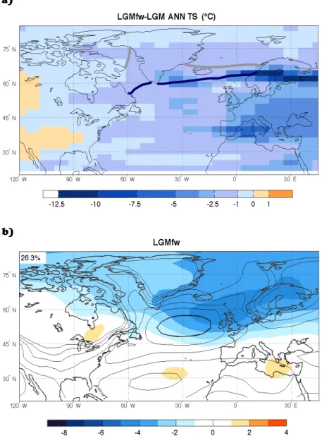
simulation, as shown in the previous sections. This result suggests that surface ocean temperatures do not greatly affect the mean atmospheric circulation in the presence of large to-pographic features such as the Laurentide ice sheet. The ad-ditional fresh water experiment (LGMfw) corroborates this result. The LGMfw experiment exhibits widespread cooling over the entire North Atlantic and an expansion of the sea ice edge relative to the full LGM (cf. Figs. 5 and 7a), but the SLP pattern and the leading pattern of SLP variability resem-ble the full LGM simulation (cf. Figs. 2 and 7b).

ghg

Fig. 5. Anomalies in annual mean surface temperature (TS) relative to the PI climate for each sensitivity experiment. Areas where the

topography difference between the experiments and the PI is greater than 500 m are masked out in white. The annual mean 50 % ice concentration line is indicated by the gray dashed line for the control (PI) experiment and the solid line for each experiment.

4 Discussion

We have presented results from sensitivity experiments car-ried out with a coupled atmosphere-ocean general circulation model showing the impact of various LGM boundary condi-tions on the mean state and variability of the atmospheric circulation. Each LGM boundary condition has been ap-plied separately to investigate its individual impact relative to a control PI simulation.

Our study shows that ice sheet topography plays a dom-inant role in altering the mean state and variability of the large-scale atmospheric circulation, particularly in the North Atlantic. This is consistent with previous model studies (Li, 2007; Li and Battisti, 2008; Pausata et al., 2009; Langen and Vinther, 2009), including those (Kageyama et al., 1999;

Justino et al., 2005) that used alternative ice sheet reconstruc-tions such as ICE-4G (Peltier, 1994). Ice sheet topography also influences SSTs, causing a widespread surface warm-ing over the North Atlantic (experiment LGMtopo). Despite this SST warming, features such as the winter 200-hPa zonal wind field, the annual mean SLP distribution and SLP vari-ability are very similar in LGMtopo and the full LGM simu-lation (Sect. 3.3).

Uncoupled AGCM studies (e.g. Rind, 1987) and studies with AGCMs coupled to a slab ocean (e.g. Manabe and Broccoli, 1985; Felzer et al., 1996, 1998) have already re-ported a warming in the presence of North American and Fennoscandian ice sheets, particularly in the regions south of the ice sheets and in the northernmost North Atlantic, east of Greenland. They attribute this localized warming to

-90 -60 -30 0 30 60 90 -8 -6 -4 -2 0 2 4 6 8 PI LGMtopo LGM Atmospheric transport -90 -60 -30 0 30 60 90 -0.5 0 0.5 1 1.5

Total Atlantic transport

-90 -60 -30 0 30 60 90 -0.5 0 0.5 1 1.5

Atlantic transport by overturning

Fig. 6. Northward heat transport (PW, vertical axis) in the

atmo-sphere (upper), in the North Atlantic ocean (middle), and by the North Atlantic overturning circulation (lower) as a function of lati-tude (horizontal axis).

thermal anticyclones (over the ice sheets), which are associ-ated with subsidence; reduced summer cloud cover; and a generally deeper Icelandic low in winter, which is associated with stronger southwesterly winds and a consequent ing in the northernmost North Atlantic. However, the warm-ing observed in our experiment (LGMtopo) is much broader than the warming observed in these previous uncoupled or partially coupled studies, suggesting that the proposed expla-nations (subsidence downstream of ice sheets and deepening of the Icelandic low) are insufficient for explaining the re-sponse in the fully coupled framework of our experiments. The increased atmosphere and ocean heat transport into the North Atlantic (Fig. 6) likely provides an additional contri-bution to the warming.

The other boundary conditions, such as GHG concen-trations and land ice albedo, have a much smaller and sometimes opposite influence to that of topography, de-pending on the season and latitude band of interest. The

main atmospheric responses to the reduced GHGs are a widespread surface cooling that is more intense at high lat-itudes (Fig. 5) and a more zonally oriented 200-hPa wind structure in the Atlantic sector relative to the control PI sim-ulation (Fig. 8). There is little change in the strength of the jet itself in LGMghg compared to PI (Fig. 3), consis-tent with the fact that there is also little change in the mid-tropospheric temperature gradients (Fig. 4). The importance of mid-tropospheric changes for determining jet strength has also been noted in future scenarios with increased GHG con-centrations, where it appears that strengthened mid-to-upper tropospheric gradients are often simulated to win out over weakened surface gradients to increase jet-level wind speeds (as shown for example in R¨ais¨anen, 2003).

While this study has corroborated the suggestion of Pausata et al. (2009) that surface ocean changes play a sec-ondary role to topography in determining the large scale atmospheric circulation features at the LGM, unresolved questions remain. In this particular coupled model (IPSL), widespread North Atlantic warming (LGMtopo) or cooling (LGMfw) along with the associated sea ice changes do not greatly affect the climatological SLP field or its leading pat-tern of variability under LGM boundary conditions. A simi-lar insensitivity of SLP and SLP variability to surface ocean changes was also found in an uncoupled atmosphere model (CAM3, Collins et al., 2006), not only under LGM bound-ary conditions but also with modern (PI) topography (Pausata et al., 2009, Fig. 6). In contrast, Byrkjedal et al. (2006) found substantial changes in LGM SLP variability associated with SST/sea ice changes, also in an uncoupled set up. Possible reasons for the discrepancy are the use of a different atmo-sphere model (ARPEGE, D´equ´e et al., 1994), or the fact that the Byrkjedal et al. (2006) experiments include large sea ice changes quite far south (down to 45◦N) in the North Atlantic compared to all the experiments in this study and in Pausata et al. (2009), all of which remain relatively ice-free south of 55◦N except in the Labrador Sea. Indeed, Kageyama et al. (1999) showed a strong link between the sea-ice edge and the upper level jet-stream in PMIP1 experiments with pre-scribed or computed (via a slab ocean) SSTs and sea ice as long as the sea ice edge was far enough south, in the mid-latitude North Atlantic.

Together with previous studies, the results presented here highlight some major challenges for model intercomparisons of LGM simulations. Pausata et al. (2009) found that SLP and SLP variability were different in LGM simulations per-formed with different coupled climate models, but seemingly not because of differences in SST/sea ice distributions (Fig. 6 in Pausata et al., 2009). This led to a speculation that sim-ulated large-scale flow characteristics in drastically altered climate states may differ from model to model because of the model-dependent treatment of the topographic bound-ary condition. The present study has reinforced the primbound-ary role of topography over the other boundary conditions in set-ting the atmospheric circulation (even when coupled ocean

a)

b)

Fig. 7. (a) Changes in the LGMfw annual mean surface temperature (TS) relative to the LGM climate and b) the leading EOF of monthly

SLP anomalies (colored shading: hPa/standard deviation of PC) using all months shown along with the SLP climatology (contours: 4 hPa interval from 1000 to 1040 hPa; higher values omitted for clarity; bold contour denotes 1016 hPa) in the North Atlantic sector for the LGMfw simulation. The annual mean 50 % sea ice concentration line is indicated by the gray line for the LGM experiment and by the blue line for the LGMfw experiment. The leading EOF of SLP variability explains 26.3 % of the total variance, as indicated.

feedbacks come into play). It has also reinforced the fact that a direct link between SST/sea ice changes and fundamental features of the atmospheric circulation is not clear in coupled LGM simulations. Given that Pausata et al. (2009) showed a similar lack of a well-defined ocean-atmosphere relation-ship for uncoupled LGM and PI simulations, it is possible that presumed links between SST and atmospheric circula-tion in a future, enhanced GHG world may be similarly ob-fuscated. Systematic studies using suites of coupled and un-coupled models are needed to further clarify the reasons for the model-dependence of the large scale circulation response in simulations of the LGM.

5 Conclusions

In this study, we analyze how gross features of the atmo-spheric general circulation are altered by each Last Glacial Maximum (LGM) boundary condition in a coupled climate model. The main findings are:

– Ice sheet topography sets many features of the SLP

field, including the location of the subtropical highs and subpolar lows, the interannual variability, and the lead-ing pattern of variability in the North Atlantic sector. Topography further controls the position, strength and

Fig. 8. Winter (November to April) 200-hPa zonal winds for the control (PI) simulation (contours: 5 m s−1interval from 5 to 50 m s−1; bold contour at 35 m s−1) and the difference (shading) between the LGMghg experiment and the control run (LGMghg-PI).

shape of the zonal wind field at 200 hPa in the North Atlantic, especially during winter, while in summer the albedo is also a leading factor.

– Applying LGM GHG and ice sheet albedo boundary

conditions to a PI simulation increases the gradient be-tween subpolar low and subtropical high SLP centers, whereas LGM topography is less important to this as-pect of atmospheric circulation in the North Atlantic sector.

– SST plays only a secondary role in setting the

climatological-mean SLP pattern, 200-hPa zonal winds, the interannual variability of SLP, or the leading pattern of SLP variability in the North Atlantic, supporting the suggestions proposed by Pausata et al. (2009).

Acknowledgements. This work is part of the ARCTREC project and funded by the Norwegian Research Council. The simulations were performed on the NEC-SX8 computer at Centre de Calcul Recherche et Technologie (CCRT), Commissariat `a l’Energie Atomique (CEA). This is publication no. A335 from the Bjerknes Centre for Climate Research.

Edited by: H. Renssen

References

Braconnot, P., Otto-Bliesner, B., Harrison, S., Joussaume, S., Pe-terchmitt, J.-Y., Abe-Ouchi, A., Crucifix, M., Driesschaert, E., Fichefet, Th., Hewitt, C. D., Kageyama, M., Kitoh, A., Lan, A., Loutre, M.-F., Marti, O., Merkel, U., Ramstein, G., Valdes, P., Weber, S. L., Yu, Y., and Zhao, Y.: Results of PMIP2 coupled simulations of the Mid-Holocene and Last Glacial Maximum –

Part 1: experiments and large-scale features, Clim. Past, 3, 261– 277, doi:10.5194/cp-3-261-2007, 2007.

Brandefelt, J. and Otto-Bliesner, B. L.: Equilibration and variabil-ity in a Last Glacial maximum climate simulation with CCSM3, Geophys. Res. Lett., 36, L19712, doi:10.1029/2009GL040364, 2009.

Byrkjedal, O., Kvamsto, N., Meland, M., and Jansen, E.: Sensitiv-ity of last glacial maximum climate to sea ice conditions in the Nordic Seas, Clim. Dynam., 26, 473–487, doi:10.1007/s00382-005-0096-2, 2006.

Chiang, J. C. H., Biasutti, M., and Battisti, D. S.: Sensitivity of the Atlantic Intertropical Convergence Zone to Last Glacial Maximum boundary conditions, Paleoceanography, 18, 1094, doi:10.1029/2003PA000916, 2003.

Collins, W. D., Rasch, P. J., Boville, B. A., Hack, J. J., McCaa, J. R., Williamson, D. L., Briegleb, B. P., Bitz, C. M., Lin, S. J., and Zhang, M. H.: The formulation and atmospheric simulation of the Community Atmosphere Model version 3 (CAM3), J. Cli-mate, 19, 2144–2161, 2006.

Czaja, A. and Frankignoul, C.: Influence of the North Atlantic SST on the atmospheric circulation, Geophys. Res. Lett., 26, 2969– 2972, 1999.

Dallenbach, A., Blunier, T., Fluckiger, J., Stauffer, B., Chappellaz, J., and Raynaud, D.: Changes in the atmospheric CH4 gradient between Greenland and Antarctica during the Last Glacial and the transition to the Holocene, Geophys. Res. Lett., 27, 1005– 1008, 2000.

D´equ´e, M., Dreveton, C., Braun, A., and Cariolle, D.: The ARPEGE/IFS atmosphere model – a contribution to the french community climate modeling., Clim. Dynam., 10, 249–266, 1994.

Felzer, B., Oglesby, R. J., Webb, T., and Hyman, D. E.: Sensitivity of a general circulation model to changes in northern hemisphere ice sheets, J. Geophys. Res.-Atmos., 101, 19077–19092, 1996. Felzer, B., Webb, T., and Oglesby, R. J.: The impact of ice sheets,

Sensi-tivity experiments with a general circulation model, Quat. Sci. Rev., 17, 507–534, 1998.

Fl¨uckiger, J., Dallenbach, A., Blunier, T., Stauffer, B., Stocker, T. F., Raynaud, D., and Barnola, J. M.: Variations in atmospheric N2O concentration during abrupt climatic changes, Science, 285,

227–230, 1999.

Frankignoul, C. and Kestenare, E.: Observed Atlantic SST anomaly impact on the NAO: An update, J. Climate, 18, 4089–4094, 2005. Hansen, J., Lacis, A., Rind, D., Russell, G., Stone, P., Fung, I., Ruedy, R., and Lerner, J.: Climate sensitivity: Analysis of feed-back mechanisms, AGU monograph, 130–163, 1984.

Hewitt, C. D. and Mitchell, J. F. B.: Radiative forcing and response of a GCM to ice age boundary conditions: cloud feedback and climate sensitivity, Clim. Dynam., 13, 821–834, 1997.

Justino, F., Timmermann, A., Merkel, U., and Souza, E. P.: Synop-tic Reorganization of Atmospheric Flow during the Last Glacial Maximum, J. Climate, 18, 2826–2846, 2005.

Kageyama, M., D’Andrea, F., Ramstein, G., Valdes, P. J., and Vautard, R.: Weather regimes in past climate atmospheric gen-eral circulation model simulations, Clim. Dynam., 15, 773–793, 1999.

Kageyama, M., Mignot, J., Swingedouw, D., Marzin, C., Alkama, R., and Marti, O.: Glacial climate sensitivity to different states of the Atlantic Meridional Overturning Circulation: results from the IPSL model, Clim. Past, 5, 551–570, doi:10.5194/cp-5-551-2009, 2009.

Kim, S. J.: The effect of atmospheric CO2 and ice sheet

to-pography on LGM climate, Clim. Dynam., 22, 639–651, doi:10.1007/s00382-004-0412-2, 2004.

Laˆın´e, A., Kageyama, M., Salas-M`elia, D., Voldoire, A., Rivi`ere, G., Ramstein, G., Planton, S., Tyteca, S., and Petershmitt, J. Y.: Northern hemisphere storm tracks during the last glacial max-imum in PMIP2 ocean-atmosphere coupled models: energetic study, seasonal cycle, precipitation, Clim. Dynam., 32, 593–614, 2009.

Langen, P. L. and Vinther, B. M.: Response in atmospheric circula-tion and sources of Greenland precipitacircula-tion to glacial boundary conditions, Clim. Dynam., 32, 1035–1054, 2009.

Li, C.: A general circulation modelling perspective on abrupt cli-mate change during glacial times, Ph.D. thesis, University of Washington, 2007.

Li, C. and Battisti, D. S.: Reduced Atlantic storminess during Last Glacial Maximum: Evidence from a coupled climate model, J. Climate, 21, 3561–3579, doi:10.1175/2007JCLI2166.1, 2008. Lynch-Stieglitz, J., Adkins, J. F., Curry, W. B., Dokken, T.,

Hall, I. R., Herguera, J. C., Hirschi, J. J. M., Ivanova, E. V., Kissel, C., Marchal, O., Marchitto, T. M., McCave, I. N., Mc-Manus, J. F., Mulitza, S., Ninnemann, U., Peeters, F., Yu, E.-F., and Zahn, R.: Atlantic meridional overturning circula-tion during the Last Glacial Maximum, Science, 316, 66–69, doi:10.1126/science.1137127, 2007.

Manabe, S. and Broccoli, A. J.: The influence of continental ice sheets on the climate of an ice-age, J. Geophys. Res.-Atmos., 90, 2167–2190, 1985.

Marti, O., Braconnot, P., Dufresne, J. L., Bellier, J., Benshila, R., Bony, S., Brockmann, P., Cadule, P., Caubel, A., Codron, F., De Noblet, N., Denvil, S., Fairhead, L., Fichefet, T., Foujols, M. A., Friedlingstein, P., Goosse, H., Grandpeix, J. Y., Guil-yardi, E., Hourdin, F., Idelkadi, A., Kageyama, M., G., K., Levy,

C., Madec, G., Mignot, J., Musat, I., Swingedouw, D., and Ta-landier, C.: Key features of the IPSL ocean atmosphere model and its sesntivity to atmospheric resolution, Clim. Dynam., 34, 1–26, 2010.

Monnin, E., Indermuhle, A., Dallenbach, A., Fluckiger, J., Stauf-fer, B., Stocker, T., Raynaud, D., and Barnola, J.: Atmospheric CO2concentrations over the last glacial termination, Science,

291, 112–114, 2001.

Otto-Bliesner, B. L., Hewitt, C. D., Marchitto, T. M., Brady, E., Abe-Ouchi, A., Crucifix, M., Murakami, S., and Weber, S. L.: Last Glacial Maximum ocean thermohaline circulation: PMIP2 model intercomparisons and data constraints, Geophys. Res. Lett., 34, L12706, doi:10.1029/2007GL029475, 2007.

Pausata, F. S. R., Li, C., Wettstein, J. J., Nisancioglu, K. H., and Battisti, D. S.: Changes in atmospheric variability in a glacial climate and the impacts on proxy data: a model intercomparison, Clim. Past, 5, 489–502, doi:10.5194/cp-5-489-2009, 2009. Peltier, W. R.: Ice Age Paleotopography, Science, 265, 195–201,

1994.

Peltier, W. R.: Global glacial isostasy and the surface of the ice-age Earth: The ICE-5G (VM2) model and GRACE, Annu. Rev. Earth Planet. Sci., 32, 111–149, doi:10.1146/annurev.earth.32.082503.144359, 2004.

R¨ais¨anen, J.: CO2-induced changes in atmospheric angular

momen-tum in CMIP2 experiments, J. Climate, 16, 132–143, 2003. Rhines, P., H¨akkinen, S., and Josey, S. A.: Is oceanic heat transport

significant in the climate system?, Springer, ch. 4, 2008. Rind, D.: Components of the ice-age circulation, J. Geophys.

Res.-Atmos., 92, 4241–4281, 1987.

Rivi`ere, G., Laˆın´e, A., Salas-M`elia, D., and Kageyama, M.: Link between Rossby Wave Breaking and the North Atlantic Oscillation-Arctic Oscillation in Present-Day and Last Glacial Maximum Climate Simulations, J. Climate, 23, 2987–3008, 2010.

Roche, D. M., Dokken, T. M., Goosse, H., Renssen, H., and We-ber, S. L.: Climate of the Last Glacial Maximum: sensitivity studies and model-data comparison with the LOVECLIM cou-pled model, Clim. Past, 3, 205–224, doi:10.5194/cp-3-205-2007, 2007.

Walker, G. T. and Bliss, E. W.: World Weather, V. Mem. R. Meteo-rol. Soc., 4, 53–83, 1932.

Watanabe, M. and Kimoto, M.: Atmosphere-ocean thermal cou-pling in the North Atlantic: A positive feedback, Q. J. R. Meteo-rol. Soc., 126, 3343–3369, 2000.

Weber, S. L., Drijfhout, S. S., Abe-Ouchi, A., Crucifix, M., Eby, M., Ganopolski, A., Murakami, S., Otto-Bliesner, B., and Peltier, W. R.: The modern and glacial overturning circulation in the At-lantic ocean in PMIP coupled model simulations, Clim. Past, 3, 51–64, doi:10.5194/cp-3-51-2007, 2007.

Wunsch, C.: Determining paleoceanographic circulations, with em-phasis on the Last Glacial Maximum, Quat. Sci. Rev., 22, 371– 385, 2003.

Yokoyama, Y., Lambeck, K., De Deckker, P., Johnston, P., and Fi-field, L. K.: Timing of the Last Glacial Maximum from observed sea-level minima, Nature, 406, 713–716, 2000.