HAL Id: hal-02416237
https://hal.archives-ouvertes.fr/hal-02416237
Submitted on 17 Dec 2019
HAL is a multi-disciplinary open access
archive for the deposit and dissemination of sci-entific research documents, whether they are pub-lished or not. The documents may come from teaching and research institutions in France or abroad, or from public or private research centers.
L’archive ouverte pluridisciplinaire HAL, est destinée au dépôt et à la diffusion de documents scientifiques de niveau recherche, publiés ou non, émanant des établissements d’enseignement et de recherche français ou étrangers, des laboratoires publics ou privés.
temporal variation of the thermal stratification in the
cold leg during emergency core cooling injection
U. Bieder, Mg. Rodio
To cite this version:
U. Bieder, Mg. Rodio. temporal variation of the thermal stratification in the cold leg during emergency core cooling injection. IHTC-16 - 16th International Heat Transfer Conference, Aug 2018, Pekin, China. �hal-02416237�
IHTC16-23148
*Corresponding Author: ulrich.bieder@cea.fr
1
TEMPORAL VARIATION OF THE THERMAL STRATIFICATION IN THE
COLD LEG DURING EMERGENCY CORE COOLING INJECTION
Ulrich Bieder*, Maria Giovanna Rodio
DEN-STMF, CEA, Université Paris-Saclay, 91191 Gif-sur-Yvette, France
ABSTRACT
The aging of the reactor pressure vessel (RPV) can be a limiting factor in life time extension of pressurized water reactors. Important thermal stresses can be generated in the RPV in the case of loss of coolant accidents. Cold emergency core cooling (ECC) water will be injected under high pressure conditions into the cold leg (horizontal pipe) and can come in contact with the hot RPV wall. This process is called pressurized thermal shock (PTS). The efficiency of the PTS is dependent on the mixing between cold ECC water and the hot coolant inventory in the cold leg and the upper downcomer (annular space). Several PTS scenarios have been analyzed experimentally in the TOPFLOW-PTS facility, situated at Helmholtz Zentrum Dresden Rossendorf (HZDR), Germany. The experimental objective was reproducing whole scenarios of PTS events under realistic small break loss of coolant accident thermal hydraulic conditions. A single phase TOPFLOW experiment is analyzed numerically by two different numerical approaches in order to get access to detailed information on the temporal development of both thermal stratification and flow behavior in the cold leg and the upper downcomer: Large Eddy Simulations with two approaches to account for thermal effects: incompressible fluid hypothesis with Boussinesq approximation and dilatable fluid hypothesis. The CEA in-house CFD code TrioCFD is used. Calculated temperature profiles in the cold leg are compared to detailed temperature measurements for a 400 s ECC injection transient. The dilatable approach reproduces well the experimental results.
KEY WORDS:
Numerical simulation and super-computing, Turbulent transport, Nonlinear thermal fluid phenomena, Nuclear energy, Thermal-hydraulics, Fluid mixing1. INTRODUCTION
The modelling of high pressure mixing of fluids at different temperatures is analysed on the example of the primary circuit of nuclear power plants. The aging of the reactor pressure vessel (RPV) can be a limiting factor in life time extension of pressurized water reactors (PWR). Important thermal stresses can be generated in the RPV in the case of loss of coolant accidents. Cold emergency core cooling (ECC) water will be injected under high pressure conditions into the cold leg and can come in contact with the hot RPV wall. This process is called pressurized thermal shock (PTS). The intensity of the PTS is dependent on the mixing between cold ECC water and the hot coolant inventory in cold leg and upper downcomer.
Low pressure mixing phenomena related to PTS have been analysed experimentally in the ROCOM test facility, situated at Helmholz Zentrum Dresden Rossendorf (HZDR), Germany [1]. Some of these experiments have been used for CFD validation, focusing on the mixing of cold ECC water with a natural-, mixed-, or forced convection flow in hot leg, downcomer and lower plenum of PWR [2]. The main attention was turned hereby to downcomer and lower plenum.
High pressure mixing phenomena related to PTS have been analysed experimentally in the TOPFLOW facility, situated at HZDR [3]. The TOPFLOW facility represents a simplified part of the primary circuit of a
IHTC16-23148
2
French 900 MWe PWR. The facility was co-financed by HZDR and three French organizations, namely Alternative and Atomic Energy Commission (CEA), Radio-protection and Nuclear Safety Institute (IRSN) and Electricity of France (EDF). The facility was built to investigate the flow behaviour in both cold leg and downcomer during ECC water injection. The objective was reproducing whole scenarios of PTS events under realistic small break loss of coolant accident thermal hydraulic conditions.
Only analysis of steady state TOPFLOW experiments have been published to date in order to validate numerical codes [3, 4], with the exception of the work of Mérigoux [5], who has analysed a transient experiment. Thus, only very limited published results exist to date on the physical and numerical analysis of unsteady mixing phenomena in the TOPFLOW facility.
PTS events are strongly influenced by the flow mixing evolution between cold and saturated water streams. In such cases, the flow mixing is incomplete and thermal stratification is created. Moreover, the backflow of hot coolant from the downcomer region to the ECC injection region was observed experimentally. This phenomenon is not completely understood to date. It is thus evident that a detailed analysis of unsteady TOPFLOW experiments is mandatory in order to have a more clear comprehension of the phenomena that influences PTS events. In this context, it is important to define the model hypothesis which are appropriate to reproduce stratification and backflow. This paper aims comparing the dilatable and incompressible modelling approach for reproducing the unsteady TOPFLOW test case PTS TSW 3-4. The objective is showing the efficacy of two hypotheses of buoyancy modelling for liquid flow at high pressure and large temperature differences thermodynamic conditions, which are typical for a PWR during ECC injection.
2. THE TOPFLOW FACILITY
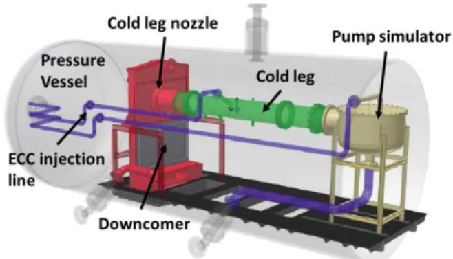
The TOPFLOW facility represents in a simplified way a part of the primary circuit of a French CPY 900 MWe PWR at a scale of 1/2.5 [1, 5]. As shown in Fig. 1, the facility consists of four principal reactor components which are placed in a pressure vessel: pump simulator, cold leg, ECC injection line and downcomer. The TOPFLOW facility allows investigating the flow behaviour in the cold leg and the downcomer under realistic thermal hydraulic conditions. The vessel can be pressurized up to 5 MPa, corresponding to a water saturation temperature of 264°C.
Since the TOPFLOW test case PTS TSW 3-4 was intended as single phase experiment, steam is only present in the upper part of downcomer in order to assure that the steam/water level was located always above the cold leg nozzle. Steam could never enter into the cold leg. Both pump simulator exits were closed and form dead branches. All water injected by the ECC line is evacuated via the downcomer outlet branch. Six thermocouple lances are used to follow the thermal stratification in the cold leg. They are mounted vertically across the centre line of the cold leg. In this paper, only the measurements of the lances LA1, LA2, LA3 and LA4 are used, each equipped with 25 thermocouples. Their axial location is given in Fig. 2.
Fig. 1 Main components of the TOPFLOW facility
located in a pressure vessel
Fig. 2 Side view of the TOPFLOW facility and
3
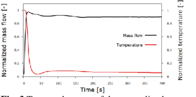
The analysed experiment was performed in the following way: In initial state, the whole facility was filled with immobile water at saturation temperature. The system pressure is at 5 MPa.
The ECC water injection was activated at t=0 s. The ECC mass flow increases linearly to reach the
maximum value at about t = 30 s.
Then, the ECC mass flow decreases non-linearly to reach the target value at about t= 100 s.
The ECC water temperature decreases to the minimum value at t = 40 s.
Then, the temperature increases to reach a local maximum at t = 90 s.
After t=100 s, the temperature is decreasing almost linearly with about 1°C per minute.
3. NUMERICAL SOLUTION OF THE CONSERVATION EQUATIONS
The TrioCFD1 is a general 3D single phase CFD code developed at CEA-Saclay [2, 6]. In the study
presented here, turbulence is treated by large eddy simulations (LES) and two approaches were tested to account for buoyancy effects, the model for incompressible fluid with the Boussinesq approximation, and the model for dilatable fluid.
3.1 Incompressible Fluid
The fluid is assumed to be Newtonian and the density is assumed to be constant. Buoyancy effects are taken into account only in the gravity term by linearizing the dependency of the density on temperature (Boussinesq’s approximation) [7]. This approach is valid in the limit of <0.1, what is not totally justified in the analyzed experiment where <0.2. The instantaneous field of the filtered velocity
u
is defined by the equation of mass conservation (eq.1) and the equation of momentum conservation (eq.2). Einstein’s notation is used.0 j j x u (1)
0 0 1 T T g x u x u x x P x u u t u i i j j i eff j i j j i i (2)The effective kinematic viscosity eff is based on the kinematic viscosity of the fluid and the kinematic
eddy viscosity defined by the sub-grid scale model SGS. Both, dynamic viscosity and thermal expansion
coefficient are taken as temperature dependent. The reference value of density 0 is taken for the lowest
temperature in the system T0.
3.2 Dilatable Fluid
The fluid is assumed to be Newtonian. The aim of the dilatable fluid model is to take into account density variations related to temperature variations and to avoid the presence of acoustic waves [8]. The dilatable fluid model is based on the hypothesis of splitting the pressure P into two parts:
1 http://www-trio-u.cea.fr/
Fig. 3 Temporal course of the normalized
temperature and mass flow in the first 400 seconds of ECC injection
IHTC16-23148
4
P(t,x)Pth(t)Ph(t,x) (3)
Ph is the hydrodynamic pressure and Pth denotes the thermodynamic pressure which is constant in the case of
the analyzed test. Thus, the density is assumed to be a function of temperature but not of the pressure and can be calculated by a simplified equation of state. The instantaneous field of the filtered velocity
u
can be predicted from the equation of mass conservation (eq.4) and the equation of momentum conservation (eq.5):0 j j x u t (4)
i i j j i eff j i h j j i i g x u x u x x P x u u t u (5)The effective dynamic viscosity eff is based on the dynamic viscosity of the fluid and the dynamic eddy
viscosity defined by the sub grid scale model SGS. The dynamic viscosity is taken as temperature dependent.
3.3 Turbulence Modelling
In large eddy simulations (LES), a filtering operation is applied to the instantaneous turbulent quantities [7] what leads to the filtered conservation equations (eqs.1, 2, 4, 5). The sub-grid-scale stress tensor ij, which
appears in the momentum equations, is calculated by using the analogy to Boussinesq’s eddy viscosity concept (filtering operation is shown by the overbar) and by introducing the sub-grid scale kinematic viscosity SGS:
ii ij i j j i SGS j i j i ij x u x u u u u u 3 1 (6)With the aim of better reproducing the transition from laminar to turbulent flow and obtaining a correct wall-asymptotic-behavior of the turbulent viscosity, the WALE sub-grid model [9] is applied.
3.4 Energy Conservation Equation
The reversible rate of internal energy change due to compression as well as viscous dissipation is not taken into account in the energy equation. In the conservation equation of the inner energy, only convection as well as molecular and turbulent diffusion is taken into account. Diffusion related to external forces, pressure gradients and thermophoresis is neglected [7]. The conservation of the internal energy is written for a constant thermodynamic pressure as:
j eff j j j p x T k x x T u t T c (7)The effective thermal conductivity keff is calculated from the thermal conductivity k, the sub-grid scale
dynamic viscosity SGS, and the turbulent Prandtl number Prt (Prt=0.7) according to keff = k + SGS/Prt. The
thermal conductivity is taken as temperature dependent whereas the specific heat capacity is taken as constant (4305 J/(kgK)).
3.5 Numerical Solution of the Conservation Equations
TrioCFD [2, 6] uses a finite volume based finite element approach on tetrahedral cells to integrate in conservative form all conservation equations over the control volumes belonging to the calculation domain. As in the classical Crouzeix–Raviart element, both vector and scalar quantities are located in the centers of the faces. The pressure, however, is located in the vertices and at the center of gravity of a tetrahedral element, as shown in [6] for the 2D case. This discretization leads to very good pressure/velocity coupling and has a very
5
dense divergence free basis. Along this staggered mesh arrangement, the unknowns, i.e. the vector and scalar values, are expressed using non-conforming linear shape-functions. The shape function for the pressure is constant for the center of the element and linear for the vertices.
A slightly stabilized 2nd order centered convection scheme [10] is applied to avoid numerical instabilities in
regions of high velocity gradients. The diffusion term is discretized by a 2nd order centered scheme. For the
incompressible fluid, the 2nd order explicit Adams-Bashforth scheme is used for time integration while for
dilatable fluid, the 1st order Euler explicit scheme is used. The time steps always respect the
Courant-Friedrichs-Levy stability criteria (CFL) of CFL < 0.8. The discretized momentum conservation equations are solved following the SOLA pressure projection method [7]. The resulting Poisson equation is solved with a conjugate gradient method using a symmetric successive over relaxation technique to improve convergence.
3.6 Setup of the calculation
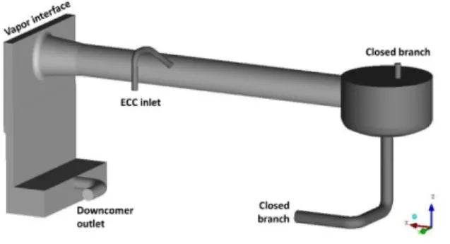
The CAD model is shown in Fig. 4. It was realized with SALOME2. Besides downcomer and cold leg, the
two closed branches and the pump simulator are modeled as these regions can represent significant reservoirs of hot fluid during the transient. The downcomer above the cold leg nozzle has been limited in height at the position 5 mm above the cold leg nozzle. The horizontal surface generated in this way represents the vapor/water interface which was located in the experiment always above the cold leg nozzle.
Fig. 4 View on the TOPFLOW geometry Fig. 5 Meshing in a vertical plane cut through ECC
line and cold leg
The CAD model was imported in “step” format in ANSYS-ICEMCFD. In a first step a surface meshing with triangles was created; then the volume was filled with tetrahedrons using the Delaunay method. The nodes on the internal walls were doubled to define boundary conditions on both sides these walls. The meshing on all solid walls is twice as fine as the maximum size of the volume mesh in order to better resolve boundary layers. A meshing of 22 million tetrahedral cells was created this way. The resulting meshing is visualized in Fig. 5 on the example of a vertical plane, cut through the ECC injection line and the cold leg.
As initial condition, the whole facility was filled with immobile saturated water at 263 °C. The calculation started with the beginning of ECC injection at t = 0 s. The following boundary conditions were used:
ECC injection: Dirichlet boundary conditions were used for mass flow and temperature at the inflow faces of the ECC line. The time dependent courses are shown in Fig. 3.
Downcomer outlet: Von Neumann conditions with an imposed pressure are applied at the outflow faces of the downcomer outlet. P = 0 Pa is used for the incompressible model and P=5 MPa for the dilatable model.
Solid walls: Standard wall functions are used to model momentum exchange between solid walls and fluid. All solid walls are treated as adiabatic.
IHTC16-23148
6
Vapor/vapor interface: This interface is located in the downcomer above the cold leg nozzle (see Fig.4). A constant flux of condensing steam is simulated by a constant vertical velocity of 0.2 mm/s.
All calculations were performed on 1008 processor cores of the HPC computer OCCIGEN of CINES, a BULL cluster of 85824 computing cores with a peak power of 3.5 Pflop/s. In order to simulate the ECC injection transient, 200 000 CPU hours were necessary to simulate 400 s with the incompressible hypothesis and 600.000 CPU hours to simulate 200 s with the dilatable hypothesis.
4. ANALYSIS OF THE TOPFLOW PTS EXPERIMENT
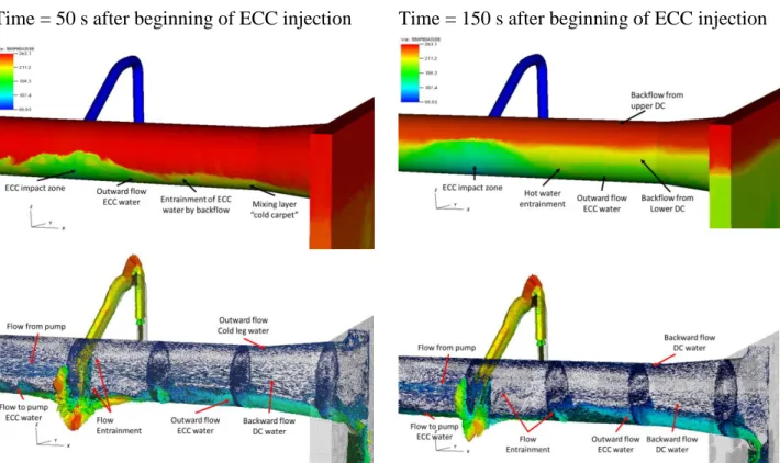
The TOPFLOW single phase experiment PTS TWS 3-4 lasted for about 3000 seconds. The first 400 seconds have been analyzed numerically as fast mixing phenomena take place in this period. Cold ECC water impacts in this period on the cold leg wall, mixes partly with the hot inventory of the cold leg and forms a stable thermal stratification in the cold leg. This flow behavior is shown in Fig.6 on the example of the temperature distribution in the early and subsequent injection phase at 50 s and 150 s after the beginning of ECC injection, respectively. The corresponding velocity fields in the center of the cold leg are added to this figure.
Time = 50 s after beginning of ECC injection
Time = 150 s after beginning of ECC injection
Fig. 6 Instantaneous temperature field at the cold leg surface and velocity field in the center of the cold leg for
the early (50s) and subsequent (150 s) injection phase
In the early injection phase at t= 50 s the jet of cold ECC water impacts on the cold leg wall and mixes efficiently by turbulence with the hot cold leg inventory. This process produces a layer of mixed ECC water which accumulates on the bottom of the cold leg due to buoyancy effects forming a cold carpet on the lower cold leg wall. The downcomer is still close to initial saturation temperature. The mixed ECC water is transported as cold streams in the directions of downcomer and pump. The impact of the cold ECC water on the cold leg wall and the formation of the outward flow in direction of the downcomer is well visible. It is also visible that cold entrained water is transported by backflow of downcomer water into the cold leg. Due to the mixing of cold ECC water with the cold leg inventory, the mass of cooled down water in the cold leg exceeds the mass of injected water. This cold inventory flows to the downcomer. In order to compensate the outward flow from the cold leg to the downcomer, a significant flow back into the cold leg from the downcomer establishes.
7
In the subsequent injection phase both cold leg and downcomer are filled with cooled down water up to the middle of the cold leg. Three temperature layers in the cold leg can be distinguished:
1. The top layer has a temperature slightly below saturation temperature. This layer is connected to the upper downcomer region which is at saturation temperature due to the presence of the water/vapor interface. The top layer is associated to backflow of hot downcomer inventory to the cold leg.
2. The lower layer representing ECC water mixed with the cold leg inventory associated to the cold carped flowing out of the cold leg.
3. The central layer with a temperature of around 180 °C associated to backflow of colder downcomer inventory to the cold leg.
It is also visible that hot water of the central layer is locally entrained into the lower layer. The backflow reaches its maximum and forms two flow regions: the center and the top of the cold leg (the cold ECC water flows out of the cold leg at the bottom of the pipe).
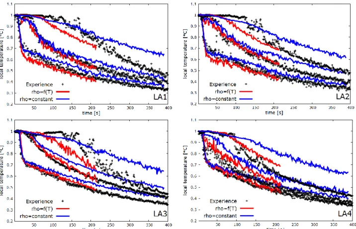
The temporal development of the fluid temperature is measured along the four vertical thermocouple lances LA1, LA2, LA3 and LA4, which are placed in the central vertical plane of the cold leg (location see Fig. 2). For each axial position, measured and calculated temperatures are compared for three selected vertical locations in the cold leg: one near the top, one in the middle and one neat the bottom. The vertical positions can easily be distinguished; the top position is represented in all figures by the hottest temperature whereas the bottom position is represented by the coldest temperatures.
Fig. 7 Comparison of measured temperature courses to values calculated with the Boussinesq hypothesis and the
dilatable approach for four thermocouple lances LA1, LA2, LA3 and LA4. Values are given near the top, in the center and near the bottom of the cold leg.
The results obtained by the dilatable hypothesis generally reproduce well the experimental data for the three vertical thermocouples locations on the four thermocouples lances. However, the incompressible hypothesis generally overestimates the fluid temperature with more important deviations from the measurements,
IHTC16-23148
8
especially for the location close to the top of the cold-leg. Significant temperature fluctuations exist already about 20 seconds after the start of ECC water injection. The stratification front reaches the cold leg center already after about 55 s of ECC injection (LA2 location). This comparison clearly shows the limitation of the Boussinesq approximation for liquids in thermodynamic conditions of high pressure and high temperature differences. In such conditions it is mandatory to include the dependency of the density on the temperature in the model hypothesis.
6. CONCLUSIONS
When cold ECC water is injected under high pressure conditions into the cold leg, this cold ECC water can come in contact with hot RPV wall initiating the so called pressurized thermal shock. The risk of a thermal shock is dependent on the mixing in the cold leg. This mixing is analyzed by CFD calculations of a TOPFLOW experiment. The TOPFLOW facility represents a simplified part of the primary circuit of a French 900 MWe PWR. Two flow hypothesis were used to take into account buoyancy effects: incompressible flow with the Boussinesq approximation and dilatable flow. Turbulence is treated by LES.
Measured temperature profiles were compared to the calculations; three elevations and four axial locations in the cold leg were selected for the comparison which shows an agreement to the experiment which is supposed to be good for dilatable modelling and still acceptable with the Boussinesq approximation. The different approaches show the same phenomenological behavior for the period analyzed.
The backflow starts in the early injection phase (first 60 s after the start of ECC injection) in the center of the cold leg. Due to the mixing of cold ECC water with the cold leg inventory, the mass of cooled down water in the cold leg exceeds the mass of injected water. This cold inventory flows to the downcomer, accelerated by buoyancy. In order to compensate the outward flow from the cold leg to the downcomer, a significant flow back into the cold leg from the downcomer establishes. This backflow reaches its maximum at about 150 s after start of ECC injection and forms two flow regions: the center and the top of the cold leg (the cold ECC water flows out of the cold leg at the bottom of the pipe).
ACKNOWLEDGMENT
This work was granted access to the HPC resources of CINES under the allocation A0012A07571 made by GENCI.
REFERENCES
[1] H.-M. Prasser, G. Grunwald, T. Höhne, S. Kliem, U. Rohde, F.P. Weiss, “Coolant mixing in a PWR - deboration transients, steam line breaks and emergency core cooling injection - experiments and analyses”, Nuclear Technology, vol. 143 (1), pp. 37-56 (2003)
[2] T. Höhne, S. Kliem, and U. Bieder, “Numerical modelling of a buoyancy-driven flow experiment at the ROCOM test facility using the CFD codes CFX and Trio_U”, Nuclear Engineering and Design, 236 (12), pp. 1309-1325, (2006)
[3] P. Apanasevich, P. Coste, B. Niceno, C. Heib, D. Lucas, “Comparison of CFD simulations on two-phase pressurized thermal shock scenarios”, Nuclear Engineering and Design, 266, pp. 112–128, (2014)
[4] P. Apanasevich, D. Lucas, M. Beyer, L. Szalinski, “CFD based approach for modelling direct contact condensation heat transfer in two-phase turbulent stratified flow”, Int. J. Therm. Sci. 95, pp.123–135, (2015)
[5] N. Mérigoux, P. Apanasevich, J.-P. Mehlhoop, D. Lucas, C. Raynaud, A. Badillo, “CFD codes benchmark on TOPFLOW-PTS experiment”. Nuclear Engineering and Design, 321, pp 288–300, (2017)
[6] P.-E. Angeli, M.-A. Puscas, G. Fauchet and A. Cartalade, “FVCA8 Benchmark for the Stokes and Navier–Stokes Equations with the TrioCFD Code—Benchmark Session”. In: Finite Volumes for Complex Applications VIII - Methods and Theoretical Aspects, New York: Springer-Verlag, pp.181-202 (2017)
[7] J. H. Ferziger and M. Peric, “Computational methods for fluid dynamics”, New York: Springer-Verlag, (2002).
[8] M. Elmo and O. Cioni, “Low Mach number model for compressible flows and application to HTR”, Nuclear Engineering and
Design, 222, pp.117–124, (2003)
[9] F. Nicoud and F. Ducros, “Subgrid-scale modelling based on the square of the velocity gradient tensor”. Flow Turbul.
Combust. 62, pp. 183–200, (1999)
[10] D. Kuzmin and S. Turek, “High-resolution FEM-TVD schemes based on a fully multidimensional flux limit”, Journal of