HAL Id: cea-02339121
https://hal-cea.archives-ouvertes.fr/cea-02339121
Submitted on 13 Dec 2019HAL is a multi-disciplinary open access archive for the deposit and dissemination of sci-entific research documents, whether they are pub-lished or not. The documents may come from teaching and research institutions in France or abroad, or from public or private research centers.
L’archive ouverte pluridisciplinaire HAL, est destinée au dépôt et à la diffusion de documents scientifiques de niveau recherche, publiés ou non, émanant des établissements d’enseignement et de recherche français ou étrangers, des laboratoires publics ou privés.
Verification and validation in LES of triple parallel jet
flow for a thermal striping investigation
P.-E. Angeli
To cite this version:
P.-E. Angeli. Verification and validation in LES of triple parallel jet flow for a thermal striping investigation. CFD4NRS-7 OECD-NEA and IAEA Workshop Application of CFD/CMFD Codes to Nuclear Reactor Safety and Design and their Experimental Validation, Sep 2018, Shanghai, China. �cea-02339121�
VERIFICATION AND VALIDATION IN LES OF TRIPLE PARALLEL JET FLOW FOR A THERMAL STRIPING INVESTIGATION
P.-E. Angeli
CEA–SACLAY, DEN/SAC/DANS/DM2S/STMF/LMSF, F-91191 Gif-sur-Yvette, France pierre-emmanuel.angeli@cea.fr
Abstract
Large Eddy Simulation (LES) consists in explicitly resolving the largest turbulent scales while the small-scale motions are taken into account by means of a subgrid-scale (SGS) model. Although it remains computationally expensive, LES seems to constitute an increasingly employed tool for engineering applications in fluid mechanics. In a nuclear context e.g., LES is a relevant approach for the numerical study and prediction of the thermal striping, which can occur during the functioning of sodium-cooled nuclear reactors and may cause some damage to the structures. Numerous experiments where three differentially heated jets mix inside a cavity were designed and conducted by the Japan Atomic Energy Agency for studying these phenomena. In order to evaluate the quality of LES using the CEA in-house TrioCFD code, a Verification and Validation study is proposed. Several LES of triple parallel jets are conducted with various grid sizes and SGS models. Following the idea of Celik et al. (2009), we look for the effective SGS kinetic energy under the form = Δ + Δ , where Δ is the grid size, the order of the numerical scheme and the order of the subgrid-scale model. In a first part, no SGS model is set and two different calculations allow to determine the values of the parameters in the above model. Then, a SGS model is added and its order of convergence is calculated. Thus, one can assess the quality of various SGS models, such as Smagorinsky and WALE. In the last part, a Validation of the results is proposed by comparing computed velocity profiles to experiment. The effects of grid resolution, SGS model and boundary conditions are discussed.
1. INTRODUCTION
Thermal striping refers to the random temperature fluctuations resulting from the mixing of non-isothermal flows and leading to thermal fatigue and crack appearance in the structures. The understanding and limitation of this phenomenon is of great interest in the nuclear reactors safety domain, and it has been the subject of various studies since the 1980s (Wood, 1980, Tokuhiro, 1999, Kimura et al., 2007). The Japan Atomic Energy Agency performed a series of experiments in water and liquid sodium to evaluate the mixing process along the jet and the transfer characteristics of temperature fluctuations from fluid to structure (Kimura et al., 2001, Miyakoshi et al., 2003). The existence of numerous associated experimental measurements gave rise to a CFD benchmark exercise which showed the overall ability of CFD codes to reproduces correctly the phenomena of interest (Angeli, 2015).
The CFD study of thermal striping requires unstationary approaches like DNS, LES or URANS to gain access to fluctuation intensity and frequency. In LES, the largest turbulent structures of the flow are calculated and the effect of small-scale motions is traduced by a subgrid-scale (SGS) model. As pointed out by Pope (2011), the ratio of resolved kinetic energy should reach 80% for a regular LES. Below the value of 80%, a LES is sometimes called VLES (Very LES) (Speziale, 1998). A value greater than 95% can be considered as a DNS (Celik, 2005). Thus, the quality of a LES can be assessed using the amount of kinetic energy in the subgrid-scales (Celik, 2009). Mathematically, this ratio can be expressed as follows:
= (1)
where is the kinetic energy of the resolved motions and the residual kinetic energy. While arises from the solution of the calculation, the estimation of requires a model. The residual kinetic energy can be related to the subgrid-scale kinematic viscosity and the local mesh size Δ:
= (2) where C is a constant depending on the SGS model. For the Smagorinsky model, Benard et al. (2016) consider the value C = 0.1 and Yoshizawa et al. (1985) the value C = 0.043, judging that a value of 0.094 is too large. Celik et al. (2009) suggest C = 0.165 and emphasizes that C can be taken within the range 0.05–0.30.
The grid convergence in LES has a particular meaning in the sense that a good LES is a DNS when the grid size tends to the Kolmogorov scale (i.e. the smallest scale in the flow). The spirit of LES to set a lower bound to the grid resolution involves the existence of a numerical viscosity which may be of the same order than the SGS viscosity (Celik et al., 2005), resulting in the deterioration of the ratio. Liu et al. (2006) note that the ratio is not necessarily improved by just reducing the grid spacing. The discrimination between the SGS contribution and the numerical discretization error is made difficult by their dependence to the grid size. Vreman et al. (1996) point out that any LES is polluted by two kinds of errors: the numerical error mentioned above, and a modelling error arising from the shortcomings of the SGS model. Following the notations of Celik et al. (2009), these two contributions write respectively, for any quantity φ:
= − (3)
= − (4)
so that the total error is:
= − = + (5)
In these definitions, is the resolved field resulting from LES on any grid, is the solution when the grid resolution tends to zero (i.e. the “exact” solution of the employed SGS model), and is the filtered DNS solution (i.e. without SGS model and when grid resolution tends to zero). It results from these definitions that if the individual errors are of opposite signs, the total error may be small (Celik et al., 2005).
Assuming that the right equations are solved, the solution of the filtered DNS should be an accurate representation of the real phenomenon. Hence the DNS solution is not needed and can be replaced by the experimental measurements. Unfortunately, obtaining the fine grid LES solution is rarely practicable in engineering applications. However it can be estimated by performing at least two simulations on different grids and using a Richardson extrapolation (Roache, 1998), based on a polynomial variation of the error:
− = ∑ Δ + Δ (6)
In this equation, the quantity is the numerical solution for the grid size ∆ and is the extrapolated solution for ∆ → 0. The assessment of the numerical and modelling errors is part of the Verification and Validation (V&V) process (Schlesinger, 1979, Roache, 1998). The Verification part copes with the resolution accuracy of the governing equations (are the equations correctly solved?), including the estimation and minimization of the discretization error . The Validation part handles the proper modelling of the physical phenomenon of interest (are the correct equations solved?) and relates to the magnitude of .
The present study is devoted to the V&V of LES of a triple parallel jet in the thermal striping context, and is focused on the hydraulic part of the phenomenon. Several LES with varying mesh sizes and SGS models are performed using the in-house CEA code TrioCFD. The case of explicit filtering is not handled. Thus the filter size and the grid size reduce to a unique parameter. The paper is divided as follows: the next section describes the experimental facility and measurement procedure. Then, the following section summarizes the numerical setup used for the simulations. Section 4 is dedicated to Verification with an estimation of the numerical errors and a discussion on the accuracy of subgrid-scale models. Section 5 relates to Validation and proposes some comparisons between CFD results and experiment with an evaluation of the discrepancies. The last section draws several conclusions and considers some perspectives.
2. EXPERIMENTAL SETUP OF THERMAL STRIPING FACILITY
The series of thermal striping experiments under consideration were performed by JAEA with varying parameters like the fluid utilized (water or liquid sodium), the velocity and the temperature of the jets. The present study is only focused on the water case under isovelocity condition. The water experiment is represented in Fig. 1. The test section is a rectangular tank limited by partition plates at front and back, and by a curved metal plate at the bottom with a raised flat part on which three nozzle outlets of rectangular cross section are designed. Their depth is 170 mm and their width is D = 20 mm. A metal test plate made of stainless steel is placed along one side wall to examine temperature fluctuations in the structure. The parallel jets are configured as one cold stream vertically flowing out from the center nozzle and two hot streams vertically flowing out from side nozzles.
Fig. 1: Sketch of the mixing cavity (left) and jet exits (right) of the triple jet facility.
The experimental conditions used in the present work are summarized in Table 1 (Tokuhiro et al., 1999, Miyakoshi et al., 2003). The velocity field is captured by Particle Image Velocimetry (PIV). The principle of PIV is recalled by Miyakoshi et al. (2003) and a schematic of the image capturing system is provided. The PIV system consists of a Nd-Yag laser, a CCD camera, a timing controller and a computer. The image size is 640 x 480 pixel and the spatial resolution is 1.3 x 1.3 mm. A field of 2520 velocity vectors is obtained with a recording time interval of 1 ms. The accuracy of image analysis is one pixel or less by using the sub-pixel method. The system has a high measurement accuracy with an order of magnitude of the velocity measurement error around 0.013 m/s, corresponding to 2.6% of the average inlet velocity.
Table 1: Experimental conditions selected for the numerical calculations. Velocity (m/s) Temperature (°C) Reynolds
Left and right jets 0.5 39 15,000
Center jet 0.5 29 13,000
The temperature in the mixing area and the thermal exchange near the adjacent steel plate are measured by movable thermocouples, yet the comparison of temperature field is not of primary interest in the present study. JAEA provided numerous velocity measurements for comparisons with the simulations, under the form of time-averaged velocity components charts at typical positions. The whole of these data represents around 150,000 measurement points.
3. NUMERICAL SETUP OF LES
3.1 Governing equations
Although the hydraulics is the phenomenon of interest here, the choice is made to solve the energy equation to account for viscosity variations due to thermal fluctuations. The dynamic viscosity is defined as a polynomial function of temperature with values ranging in the interval 0.000663–0.000814 Pa.s, being a maximal variation of 20%. Given the weak temperature difference between the jets
(Δ =10 °C), the temperature is treated as a passive scalar. In LES, the large and small-scale motions are separated by means of a spatial filtering operation denoted by an overbar. The governing equations for resolved velocity , pressure ̅ and temperature are as follows:
- Mass conservation: = 0 (7) - Momentum conservation: + = − + + + (8) - Energy conservation: + = + (9)
The SGS stress tensor in (8) is related to the SGS viscosity coefficient by the Boussinesq approximation:
≡ − = 2 ̅ + (10)
The SGS stress tensor in (9) is modeled by a simple gradient-diffusion hypothesis:
≡ − = (11)
where is the turbulent Prandtl number for which the value 0.9 is used. The rate of strain tensor in (10) is defined by:
̅ = + (12)
Two models for the SGS eddy-viscosity are considered. In the Smagorinsky model, it is expressed as:
= Δ 2 ̅ ̅ (13)
In the WALE model (Nicoud et al., 1999), the expression is:
= Δ ̅ ̅
/
̅ ̅ / ̅ ̅ / (14)
The tensor ̅ is defined by the following expression:
̅ = ̅ ̅ + Ω Ω − − Ω Ω , Ω = − (15)
The values used for the constants Cs and Cw appearing in (13) and (14) are respectively 0.18 and 0.5.
The wall shear stress and heat flux are estimated respectively with the Reichardt and Kader laws of the wall, excepted when the mesh is fine enough at walls ( < 1). In that case, no wall treatment is applied.
3.2 Numerical procedure and boundary conditions
All the calculations performed lean on a Finite Difference Volume discretization, described in Angeli (2015). The normal velocity components are located at faces and the pressure unknowns at gravity centers of the cells. This staggered arrangement avoids the creation of spurious pressure modes (“checkerboard”) compared to a collocated arrangement. The resolution is based on finite difference approximations of fluxes. A projection method is used to decouple velocity and pressure (Hirt et al., 1975): an intermediate velocity is first computed, then the mass conservation is corrected by solving a Poisson equation or pressure. The resolution of this equation uses a preconditioned conjugate gradient solver with SSOR preconditioner.
The discretization of operators consists of a second order central scheme for the diffusion term, and a QUICK scheme for the convection term. The time integration is performed by an explicit third
order Runge-Kutta scheme. A stability time step is computed at each new time step such that the Courant the number is kept lower than unity in the whole domain throughout the computation.
Short intake channels are modeled downstream the jet exits to help the boundary layer development, and uniform velocity and temperature profiles without turbulent velocity nor temperature fluctuations are applied at their inlet. The computational domain is visible in Fig. 1 at the left. The height = 0 is taken at the middle of the center intake channel. The lateral and top boundaries are outlets with a prescribed uniform reference pressure, and the other boundaries are walls. The LES solutions are time-averaged after a period of 10 physical seconds corresponding of the flow development, and over a period of 90 physical seconds in order to reach a satisfactory convergence.
3.3 Computational meshes
Three cartesian grids are constructed using blocks with non-uniform grid distribution. A preliminary RANS calculation is carried out in order to estimate the Kolmogorov scale, defined by:
= / (16)
The successive meshes are approximately refined by a factor two in the mixing region, i.e. z/D < 15. The region located at z/D > 15 downstream the nozzle exits is significantly coarsened because it is of lower interest. The main characteristics of the meshes are gathered in Table 2.
Table 2: Overview of the meshes.
Mesh 1 Mesh 2 Mesh 3 Number of elements 3,775,224 21,981,960 155,762,880 Average mesh size (mm) 1.872 1.025 0.535
Average Δ/ 27 15 8
Average time step (ms) 1.259 0.543 0.024
The range of spatial scales reachable is directly related to the mesh resolution, as shown in Fig. 2.
Fig. 2: Velocity field after two seconds in the mixing region with a 46 x 46 mm square zoom, from the mesh 1 (left) to the mesh 3 (right).
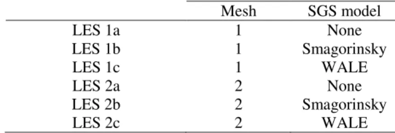
For the needs of Verification procedure, a series of LES is performed using the different grids and subgrid-scale models (Table 3). One calculation on mesh 3 is attempted but is not reported in the table, because it is still in progress.
Table 3: Summary of the LES performed for the Verification procedure. Mesh SGS model LES 1a 1 None LES 1b 1 Smagorinsky LES 1c 1 WALE LES 2a 2 None LES 2b 2 Smagorinsky LES 2c 2 WALE 4. VERIFICATION OF LES
4.1 Effective subgrid-scale kinetic energy without SGS model
In the absence of SGS model, the numerical viscosity plays implicitly the role of the SGS viscosity in the spirit of iLES (implicit LES) approaches. According to definition (3) applied to the kinetic energy as the variable φ, the numerical error on energy is approximated under the following form:
| | = − = Δ (17)
The necessity of absolute value in (17) is discussed by Celik et al. (2005): in LES, the turbulence field is not fully resolved due to the filtering process of small-scale motions. It is then expected that
is positive. However, an oscillatory convergence may happen for unclear reasons, leading to negative values of . The three unknowns in equation (17), , , and can be determined using three LES with different grid resolutions; yet this is an expensive procedure. If one assumes a value for the order of accuracy of the numerical scheme , LES 1a and LES 2a in Table 3 are sufficient. Celik et al. (2009) suggests to take = 2. According to the convergence test reported in Angeli et al. (2017) for an unstationary Navier-Stokes, = 1.5 seems to be a fair approximation with the numerical scheme employed in the present study (Fig. 3).
Fig. 3: Order of convergence for the generalized Beltrami flow. Using LES 1a and LES 2a, expression (17) leads readily to a set of two equations:
− = Δ
− = Δ (18)
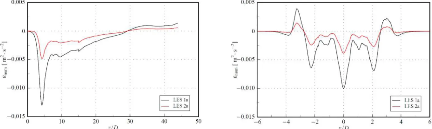
Practically, the system (18) can be numerically or analytically resolved for given values of . The numerical error for both LES are plotted in Fig. 4, confirming that it can take either positive or negative values, but the error in absolute value decreases with the grid size. However, it should be noted that the model (17) is clearly not suitable in regions where the flow is laminar, mainly because the coefficient
should depend on the local turbulence Reynolds number. Considering a uniform order of convergence may produce a negative extrapolated kinetic energy. To avoid such issues, Celik et al. (2009) suggest to apply a damping function, which has not been done here.
Fig. 4: Profiles of ε k at = 0 (left) and at ⁄ = 5 (right).
4.2 Effective subgrid-scale kinetic energy with SGS model
SGS modelling introduces an additional dissipation term which combines with the numerical dissipation. Then, the effective SGS kinetic energy is assumed to satisfy the following equation:
, = − = Δ + Δ (19)
If > (resp. < ), then the numerical error goes to zero more (resp. less) rapidly than the SGS contribution does, and the effective kinetic energy varies as Δ (resp. Δ ) when Δ → 0. If = , then both contributions have the same asymptotic behaviour. For this reason, it is postulated that equation (19) reduces to a simpler form:
, = − = Δ (20)
Using the solution computed in the previous section without SGS model, the coefficients and can be determined for Smagorinsky and WALE models using respectively LES 1b and LES 2b, LES 1c and LES 2c. The analytical solution, e.g. in the Smagorinsky case, is:
= ⁄ ln
= = (21)
Fig. 5 shows the average values of in the mixing area of the flow computed for each SGS model and various values of . It is remarkable that for the WALE model, varies roughly the same way as in the expected interval of (between 1 and 2), and remains always greater than the order of the Smagorinsky model. The interpretation is that the SGS kinetic energy decreases more rapidly with the grid size with the WALE model than with the Smagorinsky model. If =1.5, then ≈ 1.5 for the WALE model so that the numerical viscosity and SGS viscosity follow the same asymptotic behaviour. If =1.5, then ≈ 2/3 for the Smagorinsky, which is in good agreement with the evaluation made by Pope (2011) and also found by Celik et al. (2009): ~Δ ⁄ and ~Δ ⁄ (see equation (2)). This also implies that for finest grids, the effective kinetic energy is mostly contaminated by the numerical viscosity when employing the Smagorinsky model.
The definition (1) of the ratio of resolved kinetic energy is adapted under the following form: = 1 −
(22)
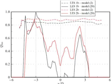
Fig. 6 shows the profiles of for the effective kinetic energy calculated according to equations (2) and (20) for the Smagorinsky model. The model (2) with = 0.043 yields a uniform ratio ranged from 80% to 90%. The unreasonable values in the central region indicates that model (20) fails. Two reasons
can be put forward. First the assumption (20) is two coarse compared to (19) where the contributions of numerical dissipation and SGS model are separated. Then the value = 1.5 is probably too pessimistic in the mixing area. The numerical convergence order is expected to increase for a decreasing local turbulent Reynolds number. The LES results on the third mesh are needed to estimate accurately the values of in the whole domain with the equation (17), as well as the other unknowns in model (19).
Fig. 5: Plot of the computed order of the SGS models in function of the numerical order of accuracy.
Fig. 6: Ratio of resolved kinetic energy for = 1.5 in the Smagorinky SGS model case, at ⁄ = 10.
5. VALIDATION OF LES
5.1 Influence of mesh size and subgrid-scale model
The flow exhibits regions of low turbulence but strong velocity gradients ( ⁄ < 2.5) and regions of strong turbulence but low velocity gradients ( ⁄ > 2.5). Fig. 7 compares the time-averaged velocity profiles at ⁄ = 2.5, ⁄ = 5 and ⁄ = 7.5 resulting from the different simulations, at midpoint between front and back plates. The profiles are normalized using the average inlet velocity = 0.5 m/s. Surprisingly, the results on mesh 1 achieve a better overall agreement with the experimental measurements. This is particularly true for the vertical component at ⁄ = 5, where the LES on the finest mesh fail at correctly reproducing the jet mixing. An attempt at explaining this behaviour is proposed in the next section. In the experiment, the velocity profiles at ⁄ = 5 are almost uniform ( ⁄ between -1 and 1), while the simulated profiles still show strong heterogeneities. As consequence, the length at which the mixing occurs is overestimated in the calculations, especially with the mesh 2. Among the SGS models, Smagorinsky yields the worst results compared to WALE and
even to the case without model. This in coherence with the well-known shortcomings of the Smagorinsky model such as: weakness in the laminar-turbulence transition and over-dissipation.
Fig. 7: Vertical and horizontal time-averaged velocity components at ⁄ = 2.5 (top), ⁄ = 5 (middle) and ⁄ = 7.5 (bottom).
5.2 Influence of wall modelling and inlet velocity conditions
The above observations are confirmed by the Table 4 where the normalized error (in norm) between the experimental and calculated points is reported for each simulation. Additional calculations using the WALE model are performed in order to evaluate the influence of wall modelling and inlet velocity profile. In the first case, the LES become wall-resolved (WR) with a refined grids at walls ( < 1) in order to account for the boundary layers without the use of wall functions. In the second case, an artificial noise is added to the velocity profile at the inlet (10% of ). A slight improvement is achieved
with these modified simulations. However, the coarsest mesh still leads to a better agreement than the finest mesh.
Table 4: Normalized norm of error between experimental and calculated values of .
Experiment Experiment LES 1a 0.1764 LES 2a 0.2371 LES 1b 0.2616 LES 2b 0.2484 LES 1c 0.1705 LES 2c 0.2384 LES 1c WR 0.1644 LES 2c WR 0.2225 LES 1c 10% 0.1684 LES 2c 10% 0.2114
Three hypotheses, not mutually exclusive, can be considered to explain the discrepancy:
- Error compensation: the numerical error and modelling error are strong with the coarse mesh but of opposite signs, leading to a relatively small total error. As a corollary, the convergence to the exact solution of the resolved equation is non-monotonic. Such a possibility is mentioned by Celik et al. (2005).
- Erroneous experimental data: this explanation seems unlikely for the two following reasons. First, it can be checked from the experimental points that they correspond to = 0.5 m/s. Second, the measurement system employed is highly accurate, as aforementioned.
- Inappropriate modelling: the equations and/or boundary conditions and/or initial conditions are unsuitable. This hypothesis is deemed to be the most probable since some tests not reported here indicate that the length at which the mixing occurs is very sensitive to whether the inlet velocity profile is flat or established. It should be confirmed by launching additional LES with established inlet velocity profiles.
6. CONCLUSIONS AND PERSPECTIVES
This study was dedicated to Verification and Validation of Large Eddy Simulations applied to triple parallel jet flow in the context of a thermal mixing investigation for nuclear reactors. In the Verification part, the numerical error was first estimated with two LES on different grids where no SGS model was set. It was shown that the kinetic energy was mostly overestimated in the mixing region of the flow, leading to a negative effective SGS kinetic energy. Then, the contribution of the SGS model was investigated. The order of convergence of the SGS kinetic energy with the Smagorinsky model was found to be in good agreement with the result of Pope (2011). The WALE model was found to converge more rapidly towards the total kinetic energy than the Smagorinsky model. However, a third LES on a finer grid is needed to refine the model, especially to compute locally the numerical order of convergence. The Validation part was made according to a set of 150,000 experimental points. The time-averaged velocity profiles were compared to the experiment and it was pointed out that the jets are mixing earlier in the experiment. Moreover, the LES on the coarsest mesh had a lower discrepancy than those on the finest mesh; the origin of this unexpected results needs to be found out. In particular, additional LES employing established inlet velocity profiles will be performed.
REFERENCES
P.-E. Angeli, “Large-Eddy Simulation of thermal striping in WAJECO and PLAJEST experiments with Trio_U”, Proc. of 16th International Topical Meeting on Nuclear Reactor Thermalhydraulics, Chicago, USA (2015).
P.-E. Angeli, “Overview of the TrioCFD code: main features, V&V procedures and typical applications to nuclear engineering”, Proc. of 16th International Topical Meeting on Nuclear Reactor
Thermalhydraulics, Chicago, USA (2015).
P.-E. Angeli et al., “FVCA8 Benchmark for the Stokes and Navier-Stokes Equations with the TrioCFD Code – Benchmark Session”. In Finite Volumes for Complex Applications VIII – Methods and
P. Benard et al., “Mesh adaptation for large-eddy simulations in complex geometries”, Int. J. Numer.
Meth. Fluids, 81, pp. 719–740 (2016).
I.B. Celik, Z.N. Cehreli and I. Yavuz, “Index of Resolution Quality for Large Eddy Simulations”, J.
Fluids Eng., 127, pp. 949–958 (2005).
I.B. Celik, M. Klein and J. Janicka, “Assessment Measures for Engineering LES Applications”, J. Fluids
Eng., 131, pp. 031102 (2009).
F. Ducros et al., “Verification and validation considerations regarding the qualification of numerical schemes for LES for dilution problems”, Nucl. Eng. Des., 240, pp. 2123–2130 (2010).
C.W. Hirt, B.D. Nichols and N.C. Romero, “SOLA – A Numerical Solution Algorithm for Transient Fluid Flows”, Technical Report LA-5852, Los Alamos National Laboratory (1975).
N. Kimura, H. Miyakoshi and H. Kamide, “Experimental investigation on transfer characteristics of temperature fluctuation from liquid sodium to wall in parallel triple-jet”, Int. J. Heat Mass Transfer, 50, pp. 2024–2036 (2007).
N. Kimura, M. Nishimura and H. Kamide, “Study on Convective Mixing for Thermal Striping phenomena – Experimental Analyses on Mixing Process in Parallel Triple-Jet and Comparisons between Numerical Methods”, Proc. of 9th International Conference on Nuclear Engineering, Nice, France (2001).
N.-S. Liu and T.-H. Shih, “Turbulence Modeling for Very Large-Eddy Simulation”, AIAA J., 44, pp. 687–697 (2006).
K. Mahesh, G. Constantinescu and P. Moin, “A numerical method for large-eddy simulation in complex geometries”, J. Comput. Phys., 197, pp. 215–240 (2004).
H. Miyakoshi et al., “Experimental Study on Thermal-Hydraulic for Thermal Striping Phenomena – Results of Temperature and Velocity Measurement among Parallel Triple Jets”, Technical Report JCN TN9410, Japan Nuclear Cycle Development Institute (2003).
J. Moureh and M. Yataghene, “Large-eddy simulation of an air curtain confining a cavity and subjected to an external lateral flow”, Comput. Fluids, 152, pp. 134–156 (2017).
F. Nicoud and F. Ducros, “Subgrid-scale stress modelling based on the square of the velocity gradient tensor”, Flow Turbul. Combust., 62, pp. 183–200 (1999).
S.B. Pope, “Ten questions concerning the large-eddy simulation of turbulent flows”, New J. Phys., 6, pp. 1–24 (2004).
S.B. Pope, “Turbulent flows”, Cambridge Univ. Press, Cambridge (2011).
P.J. Roache, “Verification and Validation in Computational Science and Engineering”, Hermosa Publishers, Albuquerque (1998).
Salome Platform, www.salome-platform.org.
S. Schlesinger, “Terminology for Model Credibility”, Simulation, 32, pp. 103–104 (1979).
C.G. Speziale, “Turbulence Modeling for Time-dependent RANS and VLES: A Review”, AIAA J., 36, pp. 173–184 (1998).
A. Tokuhiro and N. Kimura, “An experimental investigation on thermal striping. Mixing phenomena of a vertical non-buoyant jet with two adjacent buoyant jets as measured by ultrasound Doppler velocimetry”, Nucl. Eng. Des., 188, pp. 49–73 (1999).
TrioCFD, http://www-trio-u.cea.fr.
B. Vreman, B. Geurts and H. Kuerten, “Comparison of numerical schemes in Large-Eddy Simulation of the temporal mixing layer”, Int. J. Numer. Meth. Fluids, 22, pp. 297–311 (1996).
A. Yoshizawa and K. Horiuti, “A Statistically-Derived Subgrid-Scale Kinetic Energy Model for the Large-Eddy Simulation of Turbulent Flows”, J. Phys. Soc. Jpn., 54, pp. 2834–2839 (1985). D. S. Wood, “Proposal for design against thermal striping”, Nucl. Energy, 19, pp. 433–437 (1980).