Multivariate Data Analysis: The French Way
Susan Holmes∗,
Stanford University
Abstract: This paper presents exploratory techniques for multivariate data, many of them well known to French statisticians and ecologists, but few well understood in North American culture.
We present the general framework of duality diagrams which encompasses discriminant analysis, correspondence analysis and principal components and we show how this framework can be generalized to the regression of graphs on covariates.
1. Motivation
David Freedman is well known for his interest in multivariate projections [5] and his skepticism with regards to model-based multivariate inference, in particular in cases where the number of variables and observations are of the same order (see Freedman and Peters[12,13]).
Brought up in a completely foreign culture, I would like to share an alien ap- proach to some modern multivariate statistics that is not well known in North American statistical culture. I have written the paper‘the French way’with theo- rems and abstract formulation in the beginning and examples in the latter sections, Americans are welcome to skip ahead to the motivating examples.
Some French statisticians, fed Bourbakist mathematics and category theory in the 60’s and 70’s as all mathematicians were in France at the time, suffered from abstraction envy. Having completely rejected the probabilistic entreprise as useless for practical reasons, they composed their own abstract framework for talking about data in a geometrical context. I will explain the framework known as the duality diagram developed by Cazes, Caill`es, Pages, Escoufier and their followers. I will try to show how aspects of the general framework are still useful today and how much every idea from Benzecri’s correspondence analysis to Escoufier’s conjoint analysis has been rediscovered many times. Section 2.1 sets out the abstract pic- ture. Section 2.2-2.6 treat extensions of classical multivariate techniques;principal components analysis, instrument variables, cannonical correlation analysis, discrim- inant analysis, correspondence analysis from this unified view. Section 3 shows how the methods apply to the analysis of network data.
2. The Duality Diagram
Established by the French school of “Analyse des Donn´ees” in the early 1970’s this approach was only published in a few texts, [1] and technical reports [9], none of
∗Research funded by NSF-DMS-0241246
AMS 2000 subject classifications:Primary 60K35, 60K35; secondary 60K35
Keywords and phrases: duality diagram, bootstrap, correspondence analysis, STATIS, RV- coefficient
1
which were translated into English. My PhD advisor, Yves Escoufier [8][10] pub- licized the method to biologists and ecologists presenting a formulation based on his RV-coefficient, that I will develop below. The first software implementation of duality based methods described here were done inLEAS(1984) a Pascal program written for Apple II computers. The most recent implementation is the R pack- ageade-4(seeAfor a review of various implementations of the methods described here).
2.1. Notation
The data arepvariables measures onnobservations. They are recorded in a matrix X with n rows (the observations) and p columns (the variables). Dn is an nxn matrix of weights on the ”observations”, most often diagonal. We will also use a
”neighborhood” relation (thought of as a metric on the observations) defined by taking a symmetric definite positive matrix Q. For example, to standardize the variablesQcan be chosen as
Q=
1
σ21 0 0 0 ...
0 σ12 2
0 0 ...
0 0 σ12
3
0 ...
... ... ... 0 σ12
p
.
These three matrices form the essential ”triplet” (X,Q,D) defining a multivariate data analysis. As the approach here is geometrical, it is important to see that Q andD define geometries or inner products inRp andRn respectively through
xtQy=< x, y >Q x, y∈Rp xtDy=< x, y >D x, y∈Rn
From these definitions we see there is a close relation between this approach and kernel based methods, for more details see [24].Qcan be seen as a linear function fromRp toRp∗=L(Rp), the space of scalar linear functions onRp.D can be seen as a linear function fromRntoRn∗=L(Rn). Escoufier[8] proposed to associate to a data set an operator from the space of observationsRp into the dual of the space of variables Rn∗. This is summarized in the following diagram [1] which is made commutative by definingV andW as XtDX andXQXtrespectively.
R
p∗−−→
X
R
nQ x
y
V D
y
x
W
R
p←−−
Xt
R
n∗This is known as the duality diagram because knowledge of the eigendecompo- sition of XtDXQ = V Q leads to that of the dual operator XQXtD. The main consequence is an easy transition between principal components and principal axes
as we will see in the next section. The terms duality diagram or triplet are often used interchangeably.
Notes:
1. Suppose we have data and inner products defined byQand D: (x, y)∈Rp×Rp7−→xtQy=< x, y >Q∈R (x, y)∈Rn×Rn7−→xtDx=< x, y >D∈R
We say an operatorO isB-symmetric if< x, Oy >B=< Ox, y >B, or equiv- alently BO = OtB. The duality diagram is equivalent to three matrices (X,Q,D) such that X isn×pand QandD are symmetric matrices of the right size (Qisp×pand D isn×n). The operators defined asXQtXD=W D andXtDXQ=V Qare called the characteristic operators of the diagram [8], in particularV QisQ-symmetric andW DisD-symmetric.
2. V = XtDX will be the variance-covariance matrix if X is centered with regards to (D, X0D1n= 0).
3. There is an important symmetry between the rows and columns ofX in the diagram, and one can imagine situations where the role of observation or variable is not uniquely defined. For instance in microarray studies the genes can be considered either as variables or observations. This makes sense in many contemporary situations which evade the more classical notion of n observations seen as a random sample of a population. It is certainly not the case that the 30,000 probes are a sample of genes since these probes try to be an exhaustive set.
2.1.1. Properties of the Diagram
Here are some of the properties that prove useful in various settings:
• Rank of the diagramX, Xt, V QandW Dall have same rank which will usually be smaller than bothnandp.
• ForQ andD symmetric matrices V Qand W Dare diagonalisable and have the same eigenvalues. We note them in decreasing order
λ1≥λ2≥λ3≥. . .≥λr≥0≥ · · · ≥0.
• Eigendecomposition of the Diagram:
V QisQsymmetric, thus we can findZ such that
V QZ=ZΛ, ZtQZ=Ip, where Λ =diag(λ1, λ2, . . . , λp) (2.1) In practical computations, we start by finding the Cholesky decompositions ofQandD, which exist as long as these matrices are symmetric and positive definite, call theseHtH =Q and KtK =D. Here H and K are triangular.
Then we use the singular value decomposition ofKXH:
KXH=U STt, withTtT =Ip, UtU =In, S diagonal
. ThenZ = (H−1)tT satisfies (2.1) with Λ =S2. The renormalized columns ofZ,A=SZ are called the principal axes and satisfy:
AtQA= Λ
Similarly, we can defineL=K−1U that satisfies
W DL=LΛ, LtDL=In, where Λ =diag(λ1, λ2, . . . , λr,0, . . . ,0). (2.2) C=LS is usually called the matrix of principal components. It is normed so that
CtDC = Λ.
• Transition Formulæ: Of the four matrices Z, A, L and C we only have to compute one, all others are obtained by the transition formulæprovided by the duality property of the diagram.
XQZ=LS=C XtDL=ZS =A
• TheT race(V Q) =T race(W D) is often called the inertia of the diagram, (in- ertia in the sense of Huyghens inertia formula for instance). The inertia with regards to a pointAof a cloud ofpi-weighted points beingPn
i=1pid2(xi, a).
When we look at ordinary PCA withQ=Ip,D=n1In, and the variables are centered, this is the sum of the variances of all the variables, if the variables are standardizedQis the diagonal matrix of inverse variances, the intertia is the number of variablesp.
2.2. Comparing Two Diagrams: the RV coefficient
Many problems can be rephrased in terms of comparison of two ”duality diagrams”
or put more simply, two characterizing operators, built from two ”triplets”, usually with one of the triplets being a response or having constraints imposed on it. Most often what is done is to compare two such diagrams and try to get one to match the other in some optimal way.
To compare two symmetric operators there is either a vector covariance covV(O1, O2) =T r(Ot1O2) or their vector correlation[8]
RV(O1, O2) = T r(O1O2) pT r(O1tO1)tr(Ot2O2) If we were to compare the two triplets Xn×1,1,1nIn
and Yn×1,1,n1In
we would haveRV =ρ2.
P CAcan be seen as finding the matrixY which maximizes of theRV coefficient between characterizing operators that is between (Xn×p, Q, D) and (Yn×q, I, D), under the constraint thatY be of rankq < p.
RV XQXtD, Y YtD
= T r(XQXtDY YtD) q
T r(XQXtD)2T r(Y YtD)2
This maximum is attained where Y is chosen as the first q eigenvectors of XQXtD normed so thatYtDY = Λq. The maximumRV is
RV max= sPq
i=1λ2i Pp
i=1λ2i.
Of course, classical PCA has D = identity,Q= n1 identity but the extra flexibility is often useful. We define the distance between triplets (X, Q, D) and (Z, Q, M)
whereZ is alson×pas the distance deduced from the RV inner product between operatorsXQXtDandZM ZtD. In fact, the reason the French like this scheme so much is that most linear methods can be reframed in these terms. We will give a few examples such as Principal Component Analysis(ACP in French), Correspon- dence Analysis (AFC in French), Discriminant Analysis (AFD in French), PCA with regards to instrumental variable (ACPVI in French) and Canonical Correla- tion Analysis (AC).
2.3. Explaining one diagram by another
Principal Component Analysis with respect to Instrumental Variables was a tech- nique developed by C.R. Rao [25] to find the best set of coefficients in multivariate regression setting where the response is multivariate, given by a matrixY. In terms of diagrams and RV coefficients this problem can be rephrased as that of finding M to associate to X so that (X,M,D) isas close as possible to (Y,Q,D) in the RV sense.
The answer is provided by definingM such that Y QYtD=λXM XtD.
If this is possible then the two eigendecompositions of the triplet give the same answers. We simplify notation by the following abbreviations:
XtDX=Sxx YtDY =Syy XtDY =Sxy andR=Sxx−1SxyQSyxSxx−1. Then
kY QYtD−XM XtDk2=kY QYtD−XRXtDk2+kXRXtD−XM XtDk2 The first term on the right hand side does not depend onM, and the second term will be zero for the choiceM =R.
In order to have rankq <min (rank (X), rank (Y)) the optimal choice of a posi- tive definite matrixM ofM =RBBtRwhere the columns ofBare the eigenvectors ofXtDXRwith 1:
B = 1
√λ1
β1, . . . 1 pλqβq
!
XtDXRβk= λkβk
βktRβk= λk, k= 1. . . q λ1> λ2> . . . > λq
The PCA with regards to instrumental variables of rankqis equivalent to the PCA of rankqof the triplet (X, R, D)
R=Sxx−1SxyQSyxS−1xx. 2.4. One Diagram to replace Two Diagrams
Canonical correlation analysis was introduced by Hotelling[18] to find the common structure in two sets of variablesX1 and X2 measured on the same observations.
This is equivalent to merging the two matrices columnwise to form a large matrix withnrows andp1+p2 columns and taking as the weighting of the variables the matrix defined by the two diagonal blocks (X1tDX1)−1and (X2tDX2)−1
Q=
(X1tDX1)−1 0
0 (X2tDX2)−1
Rp1∗ −−−−→
X1 Rn
Ip1
x
yV1 D
y
x
W1 Rp1 ←−−−−
Xt1 Rn∗
Rp2∗ −−−−→
X2 Rn
Ip2
x
yV2 D
y
x
W2 Rp2 ←−−−−
X2t Rn∗
Rp1+p2∗ −−−−−→
[X1;X2] Rn
Q
x
yV D
y
x
W Rp1+p2 ←−−−−−−
[[X1;X2]t Rn∗
This analysis gives the same eigenvectors as the analysis of the triple
(X2tDX1,(X1tDX1)−1,(X2tDX2)−1) also known as the canonical correlation analy- sis ofX1 andX2.
2.5. Discriminant Analysis
If we want to find linear combinations of the original variablesXn×p that charac- terize the best the group structure of the points given by a zero/one group coding matrixY, with as many columns as groups, we can phrase the problem as a duality diagram. Suppose that the observations are given individual weights in the diagonal matrixD, and that the variables are centered with regards to these weights.
LetAbe theq×pmatrix of group means in each of thepvariables. This satisfies YtDX = ∆Y1qA where ∆Y is the diagonal matrix of group weights.
The variance covariance matrix will be denotedT =XtDX, with elements tjk=cov(xj, xk) =
n
X
i=1
di(xij−x¯j)(xik−x¯k) . The between group variance-covariance is
B =At∆YA.
The duality diagram for linear discriminant analysis is
R
p∗−−→
X
R
nT−1 x
yB ∆Y
y
x
AT−1At
R
p←−−
Xt
R
n∗Corresponding to the triplet (A,T−1,∆Y), because (XtDY)∆−1Y (YtDX) =At∆YA this gives equivalent results to the triplet (YtDX,T−1,∆−1Y ).
The discriminating variables are the eigenvectors of the operator At∆YAT−1
They can also be seen as the PCA with regards to instrumental variables of (Y,∆−1, D) with regards to (X, M, D).
2.6. Correspondence Analysis
Correspondence analysis can be used to analyse several types of multivariate data.
All involve some categorical variables. Here are some examples of the type of data that can be decomposed using this method:
• Contingency Tables (cross-tabulation of two categorical variables)
• Multiple Contingency Tables (cross-tabulation of several categorical vari- ables).
• Binary tables obtained by cutting continuous variables into classes and then recoding both these variables and any extra categorical variables into 0/1 tables, 1 indicating presence in that class. So for instance a continuous variable cut into three classes will provide three new binary variables of which only one can take the value one for any given observation.
To first approximation, correspondence analysis can be understood as an extension of principal components analysis (PCA) where the variance in PCA is replaced by aninertia proportional to theχ2 distance of the table from independence. CA decomposes this measure of departure from independence along axes that are or- thogonal according to a χ2 inner product. If we are comparing two categorical variables, the simplest possible model is that of independence in which case the counts in the table would obey approximately the margin products identity. For an m×p contingency table N with n = Pm
i=1
Pp
j=1nij = n·· observations and associated to the frequency matrix
F=N n Under independence the approximation
nij
=. ni·
n n·j
n n can also be written:
N .
=crtn where
r= 1
nN1p is the vector of row sums ofF andct= 1
nN01mare the column sums The departure from independence is measured by theχ2 statistic
X2=X
i,j
[(nij−ni·
n
n·j n n)2 ni·n·j
n2 n ]
Under the usual validity assumptions that the cell countsnij are not too small, this statistic is distributed as aχ2with (m−1)(p−1) degrees of freedom if the data are independent. If we do not reject independence, there is no more to be said about the table, no interaction of interest to analyse. There is in fact no ‘multivariate’
effect.
On the contrary if this statistic is large, we decompose it into one dimensional components.
Correspondence analysis is equivalent to the eigendecomposition of the triplet (X,Q,D) with
X=D−1r FD−1c −1t1,Q=Dc,D=Dr
Dc= diag(c),Dr= diag(r) X0Dr1m= 1p, the average of each column is one.
Notes:
1. Consider the matrix Dr−1FDc−1 and take the principal components with regards to the weightsDrfor the rows andDcfor the columns.
The recentered matrixDr−1FDc−1−10m1phas a generalized singular value decomposition
Dr−1FDc−1−10m1p=USV0, withU0DrU=Im,V0DcV=Ip having total inertia:
Dr(Dr−1FDc−1−10m1p)0Dc(Dr−1FDc−1−10m1p) =X2 n 2. PCA of the row profilesFDr−1
, taken with weight matrixDcwith the metric Q=Dc−1.
3. Notice that
X
i
fi·( fij fi·f·j
−1) = 0 the row and columns profiles are centered
X
j
fj˙( fij
fi·f·j −1) = 0
This method has been rediscovered many times, the most recently by Jon Klein- berg’s in his method for analysing Hubs and Authorities [19], see Fouss, Saerens and Renders, 2004[11] for a detailed comparison.
In statistics the most commonplace use of Correspondence Analysis is in ordina- tion or seriation, that is , the search for a hidden gradient in contingency tables. As an example we take data analysed by Cox and Brandwood [4] and [6] who wanted to seriate Plato’s works using the proportion of sentence endings in a given book, with a given stress pattern. We propose the use of correspondence analysis on the table of frequencies of sentence endings, for a detailed analysis see Charnomordic and Holmes[2].
The first 10 profiles (as percentages) look as follows:
Rep Laws Crit Phil Pol Soph Tim UUUUU 1.1 2.4 3.3 2.5 1.7 2.8 2.4 -UUUU 1.6 3.8 2.0 2.8 2.5 3.6 3.9 U-UUU 1.7 1.9 2.0 2.1 3.1 3.4 6.0 UU-UU 1.9 2.6 1.3 2.6 2.6 2.6 1.8 UUU-U 2.1 3.0 6.7 4.0 3.3 2.4 3.4 UUUU- 2.0 3.8 4.0 4.8 2.9 2.5 3.5 --UUU 2.1 2.7 3.3 4.3 3.3 3.3 3.4 -U-UU 2.2 1.8 2.0 1.5 2.3 4.0 3.4 -UU-U 2.8 0.6 1.3 0.7 0.4 2.1 1.7 -UUU- 4.6 8.8 6.0 6.5 4.0 2.3 3.3 ...etc (there are 32 rows in all)
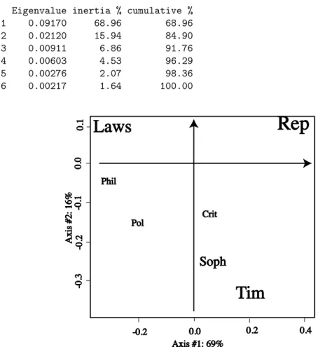
The eigenvalue decomposition (called the scree plot) of the chisquare distance matrix (see [2]) shows that two axes out of a possible 6 (the matrix is of rank 6) will provide a summary of 85% of the departure from independence, this suggests that a planar representation will provide a good visual summary of the data.
Eigenvalue inertia % cumulative %
1 0.09170 68.96 68.96
2 0.02120 15.94 84.90
3 0.00911 6.86 91.76
4 0.00603 4.53 96.29
5 0.00276 2.07 98.36
6 0.00217 1.64 100.00
Tim
Laws Rep
Soph
Phil
Pol Crit
Axis #1: 69%
Axis #2: 16%
-0.2 0.0 0.2 0.4
0.0-0.2-0.3-0.10.1
Figure 1: Correspondence Analysis of Plato’s Works
We can see from the plot that there is a seriation that as in most cases follows a parabola or arch[16] from Laws on one extreme being the latest work and Republica being the earliest among those studied.
3. From Discriminant Analysis to Networks
Consider a graph with vertices the members of a group and edges if two members interact. We suppose each vertex comes with an observation vectorxi, and that each has the same weight n1, In the extreme case of discriminant analysis, the graph is supposed to connect all the points of a group in a complete graph, and be discon- nected from the other observations. Discriminant Analysis is just the explanation of this particular graph by linear combinations of variables, what we propose here is to extend this to more general graphs in a similar way. We will suppose all the observations are the nodes of the graph and each has the same weight n1. The basic
decomposition of the variance is written cov(xj, xk) =tjk = 1
n
n
X
i=1
(xij−x¯j)(xik−x¯k) Call the group means ¯xgj = 1
ng
X
i∈Gg
xij, g= 1. . . q X
i∈Gg
(xij−x¯gj)(¯xgj−x¯k) = (¯xgj−x¯k)X
i∈Gg
(xij−x¯gj) = 0 Huyghens formula tjk=wjk+bjk
Wherewjk =
q
X
g=1
X
i∈Gg
(xij−x¯gj)(xik−x¯gk)
andbjk =
q
X
g=1
ng
n (¯xgj−x¯j)(¯xgk−x¯k) T = W +B
As we showed above, linear discriminant analysis finds the linear combinations a such that aattBaT a is maximized. This is equivalent to maximizing the quadratic form atBain a, subject to the constraintatT a= 1. As we saw above, this is solved by the solution to the eigenvalue problem
Ba=λT aor T−1Ba=λa if T−1 exists
then a0Ba = λa0T a = λ. We are going to extend this to graphs by relaxing the group definition to partition the variation into local and global components 3.1. Decomposing the Variance into Local and Global Components Lebart was a pioneer in adapting the eigenvector decompositions to cater to spatial structure in the data (see [20,21,22]).
cov(xj, xk) = 1 n
n
X
i=1
(xij−x¯j)(xik−x¯k)
= 1
2n2
n
X
i=1 n
X
i0=1
(xij−xi0j)(xik−xi0k)
var(xj) = 1 2n2
X
(i,i0)∈E
(xij−xi0j)2+ X
(i,i0)/∈E
(xij−xi0j)2
If we callM is the incidence matrix of the directed graph:mij = 1 ifipoints toj.
Suppose for the time being thatM is symmetrical (the graph is undirected). The degree of vertexiismi=Pn
i0=1mii0. We take the convention that there are no self
loops. Then another way of writing the variance formula is
var(xj) = 1 2n2
n
X
i=1 n
X
i0=1
mii0(xij−xi0j)2+ X
(i,i0)/∈E
(xij−xi0j)2
varloc(xj) = 1 2m
n
X
i=1 n
X
i0=1
mii0(xij−xi0j)2
wherem =
n
X
i=1 n
X
i0=1
mii0
The total variance is the variance of the complete graph. Geary’s ratio [14] is used to see whether the variablexjcan be considered as independent of the graph structure.
If the neighboring values ofxj seem correlated then the local variance will only be an underestimate of the variance:
G=c(xj) =varloc(xj) var(xj)
Call D the diagonal matrix with the total degrees of each node in the diagonal D=diag(mi).
For all variables taken together, j = 1, . . . p note the local covariance matrix V = 2m1 Xt(D−M)X, if the graph is just made of disjoint groups of the same size, this is proportional to the W within class variance-covariance matrix. The proportionality can be accomplished by taking the average of the sum of squares to the average of the neighboring nodes ([23]). We can generalize the Geary index to account for irregular graphs coherently. In this case we weight each node by its degree. Then we can write the Geary ratio for any n-vector x as
c(x) =xt(D−M)x
xtDx , D=
m1 0 0 0
m2 0 0 ... . .. ... . . . 0 0 mn
We can ask for the coordinate(s) that are the most correlated to the graph structure then if we want to minimize the Geary ratio, choosexsuch that c(x) is minimal, this is equivalent to minimizingxt(D−M)xunder the constraintxtDx= 1. This can be solved by finding the smallest eigenvalueµwith eigenvectorxsuch that:
(D−M)x = µDx D−1(D−M)x = µx (1−µ)x=D−1M x
This is exactly the defining equation of the correspondence analysis of the matrix M. This can be extended to as many coordinates as we like, in particular we can take the first 2 largest eigenvectors and provide the best planar representation of the graph in this way.
3.2. Regression of graphs on node covariates
The covariables measured on the nodes can be essential to understanding the fine structure of graphs. We callXthen×pmatrix of measurements at the vertices of the
graph; they may be a combination of both categorical variables (gene families, GO classes) and continuous measurements (expression scores). We can use the PCAIV method defined in section 2 to the eigenvectors of the graph defined above. This provides a method that uses the covariates inX to explain the graph. To be more precise, given a graph (V, E) with adjacency matrixM, define the Laplacian
L=D−1(M −I) D=diag(d1, d2, . . . , dn) diagonal matrix of degrees Using the eigenanalysis of the graph, we can summarize the graph with a few variables, the first few relevant eigenvectors of L, these can then be regressed on the covariates using Principal Components with respect to Instrumental Variables [25] as defined above to find the linear combination of node covariates that explain the graph variables the best.
Appendix A: Resources A.1. Reading
There are few references in English explaining the duality/operator point of view, apart from the already cited references of Escoufier[8,10]. Fr´ederique Gla¸con’s PhD thesis[15] (in French) clearly lays out the duality principle before going on to ex- plain its application to the conjoint analysis of several matrices, or data cubes. The interested reader fluent in French could also consult any one of several Masters level textbooks on the subject for many details and examples:
Brigitte Escofier and J´erˆome Pag`es[7] have a textbook with many examples, al- though their approach is geometric, they do not delve into the Duality Diagram, more than explaining on page 100 its use in transition formula between eigenbases of the different spaces.
[22] is one of the broader books on multivariate analyses, making connections be- tween modern uses of eigendecomposition techniques, clustering and segmentation.
This book is unique in its chapter on stability and validation of results (without going as far as speaking of inference).
Caillez and Pag`es [1] is hard to find, but was the first textbook completely based on the diagram approach, as was the case in the earlier literature they use transposed matrices.
A.2. Software
The methods described in this article are all available in the form ofR packages which I recommend. The most complete package is ade4[3] which covers almost all the problems I mention except that of regressing graphs on covariates, however a complete understanding of the duality diagram terminology and philosophy is necessary as these provide the building blocks for all the functions in the form a class called dudi (this actually stands for duality diagram). One of the most important features in all the‘dudi.*’functions is that when the argumentscannf is at its default valueTRUEthe first step imposed on the user is the perusal of the screeplot of eigenvalues. This can be very important, as choosing to retain 2 values by default before consulting the eigenvalues can lead to the main mistake that can be made when using these techniques: the separation of two close eigenvalues. When two eigenvalues are close the plane will be stable, but not each individual axis or
principal component resulting in erroneous results if for instance the 2nd and 3rd eigenvalues were very close and the user chose to take 2 axes[17].
Another useful addition also comes from the ecological community and is called vegan. Here is a list of suggested functions from several packages:
• Principal Components Analysis (PCA) is available inprcompand princomp in the standard packagestatsas pcain veganand asdudi.pcain ade4.
• Two versions of PCAIV are available, one is called Redundancy Analysis (RDA) and is available asrdain veganandpcaivin ade4.
• Correspondence Analysis (CA) is available inccainvegan and asdudi.coa inade4.
• Discriminant analysis is available asldainstats, as discriminin ade4
• Canonical Correlation Analysis is available incancorin stats (Bewarecca inade4 is Canonical Correspondence Analysis).
• STATIS (Conjoint analysis of several tables) is available inade4.
Acknowledgements
I would like to thank Elizabeth Purdom for discussions about multivariate analy- sis, Yves Escoufier for reading this paper and teaching much about Duality over the years, and Persi Diaconis for suggesting the Plato data in 1993 and for many conversations about the American way. This work was funded under the NSF DMS award 0241246.
References
[1] F. Cailliez and J. P. Pages.,Introduction `a l’analyse des donn´es., SMASH, Paris, 1976.
[2] B. Charnomordic and S. Holmes, Correspondence analysis for microar- rays, Statistical Graphics and Computing Newlsetter, 12 (2001).
[3] D. Chessel, A. B. Dufour, and J. Thioulouse., The ade4 package - i:
One-table methods., R News, 4 (2004), pp. 5–10.
[4] D. R. Cox and L. Brandwood, On a discriminatory problem connected with the works of plato, J. Roy. Statist. Soc. Ser. B, 21 (1959), pp. 195–200.
[5] P. Diaconis and D. Freedman,Asymptotics of graphical projection pursuit, The Annals of Statistics, 12 (1984), pp. 793–815.
[6] P. Diaconis and J. Salzmann,Projection pursuit for Discrete Data, IMS, 2006, ch. tba, p. tba.
[7] B. Escofier and J. Pag`es, Analyse factorielles simples et multiples : Ob- jectifs, m´ethodes et interpr´etation, Dunod, 1998.
[8] Y. Escoufier, Operators related to a data matrix., in Recent developments in Statistics., J. e. a. Barra, ed., North Holland,, 1977, pp. 125–131.
[9] ,Cours d’analyse des donn´ees, Cours Polycopi´e 7901, IUT, Montpellier, 1979.
[10] , The duality diagram: a means of better practical applications, in De- velopment. in numerical ecology., P. In Legendre and L. Legendre, eds., 1987, pp. 139–156.
[11] F. Fouss, J.-M. Renders, and M. Saerens, Some relationships between Kleinberg’s hubs and authorities, correspondence analysis, and thesalsaalgo- rithm, in JADT 2004, International Conference on the Statistical Analysis of Textual Data, Louvain-la-Neuve, 2004, pp. 445–455.
[12] D. A. Freedman and S. C. Peters, Bootstrapping a regression equation:
Some empirical results, Journal of the American Statistical Association, 79 (1984), pp. 97–106.
[13] ,Bootstrapping an econometric model: Some empirical results, Journal of Business & Economic Statistics, 2 (1984), pp. 150–158.
[14] R. Geary, The contiguity ratio and statistical mapping., The Incorporated Statistician, 5 (1954), pp. 115–145.
[15] F. Glac¸on,Analyse conjointe de plusieurs matrices de donn´ees. Comparaison de diff´erentes m´ethodes., PhD thesis, Grenoble, 1981.
[16] M. Hill and H. Gauch, Detrended correspondence analysis, an improved ordination technique, Vegetatio, 42 (1980), pp. 47–58.
[17] S. Holmes,Outils Informatiques pour l’Evaluation de la Pertinence d’un Re- sultat en Analyse des Donn´ees, PhD thesis, Montpellier, USTL, 1985.
[18] H. Hotelling,Relations between two sets of variables., Biometrika, 28 (1936), pp. 321–327.
[19] J. M. Kleinberg,Hubs, authorities, and communities, ACM Comput. Surv., 31 (1999), p. 5.
[20] L. Lebart,Traitement des Donn´ees Statistiques, Dunod, Paris, 1979.
[21] L. Lebart, A. Morineau, and K. M. Warwick, Multivariate Descriptive Statistical Analysis, Wiley, 1984.
[22] L. Lebart, M. Piron, and A. Morineau,Statistique exploratoire multidi- mensionnelle, Dunod, Paris, France, 2000.
[23] A. Mom, M´ethodologie statistique de la classification des r´eseaux de trans- ports., PhD thesis, Montpellier, USTL, 1988.
[24] E. Purdom,Comparative Multivariate Methods, PhD thesis, Stanford Univer- sity, Sequoia Hall, Stanford, CA 94305., 2006.
[25] C. R. Rao, The use and interpretation of principal component analysis in applied research., Sankhya A, 26 (1964), pp. 329–359.
Sequoia Hall, Stanford, CA 94305 E-mail:[email protected]