Improving the quantification of land cover pressure on stream ecological status at the riparian scale using High Spatial Resolution Imagery

HAL Id: hal-00671408

https://hal.archives-ouvertes.fr/hal-00671408

Submitted on 17 Feb 2012

HAL is a multi-disciplinary open access

archive for the deposit and dissemination of

sci-entific research documents, whether they are

pub-lished or not. The documents may come from

teaching and research institutions in France or

abroad, or from public or private research centers.

L’archive ouverte pluridisciplinaire HAL, est

destinée au dépôt et à la diffusion de documents

scientifiques de niveau recherche, publiés ou non,

émanant des établissements d’enseignement et de

recherche français ou étrangers, des laboratoires

publics ou privés.

Spatial Resolution Imagery

T. Tormos, P. Kosuth, S. Durrieu, B. Villeneuve, J.G. Wasson

To cite this version:

T. Tormos, P. Kosuth, S. Durrieu, B. Villeneuve, J.G. Wasson. Improving the quantification of

land cover pressure on stream ecological status at the riparian scale using High Spatial

Resolu-tion Imagery. Physics and Chemistry of The Earth, Elsevier, 2011, 36 (12), p. 549 - p. 559.

�10.1016/j.pce.2010.07.012�. �hal-00671408�

Improving the quantification of land cover pressure on stream ecological

status at the riparian scale using High Spatial Resolution Imagery

T. Tormos a,*_{, P. Kosuth} a_{, S. Durrieu} a_{, B. Villeneuve} b_{, J.G. Wasson}†b

a Remote Sensing & Geo-information for Environment and Land Management, cemagref, 500 rue Jean François Breton, 34093

Montpellier, France

b Laboratory of Quantitative Hydroecology, cemagref, 3 bis quai Chauveau, CggP 220, 69336 cedex 09, Lyon, France

Abstract

The aim of this paper is to demonstrate the interest of High Spatial Resolution Imagery (HSRI) and the limits of coarse land cover data such as CORINE Land Cover (CLC), for the accurate characterization of land cover structure along river corridors and of its functional links with freshwater ecological status on a large scale. For this purpose, we compared several spatial indicators built from two land cover maps of the Herault river corridor (southern France): one derived from the CLC database, the other derived from HSRI. The HSRI-derived map was obtained using a supervised object-based classification of multi-source remotely-sensed images (SPOT 5 XS-10 m and aerial photography-0.5 m) and presents an overall accuracy of 70 %. The comparison between the two sets of spatial indicators highlights that the HSRI-derived map allows more accuracy in the quantification of land cover pressures near the stream: the spatial structure of the river landscape is finely resolved and the main attributes of riparian vegetation can be quantified in a reliable way. The next challenge will consist in developing an operational methodology using HSRI for large-scale mapping of river corridor land cover,, for spatial indicator computation and for the development of related pressure/impact models, in order to improve the prediction of stream ecological status.

Keywords: Stream ecological status; Riparian Corridor; River Corridor, High Spatial Resolution imagery; Spatial Indicators; Water Framework Directive

1. Introduction

Preservation and restoration of the ecological quality of river ecosystems is a major social issue. It is the aim of several European Community actions such as the Water Framework Directive (WFD 2000) that provides a new legislative framework to manage, protect and restore surface waters in Europe. Prior to the definition of efficient management and restoration strategies and actions, an improved understanding of the mechanisms through which land use impacts stream ecosystems is needed (Allan, 2004).

Landscape ecology emphasizes the interaction between spatial patterns and ecological processes (Turner, 1989) and provides relevant conceptual and technical tools to establish relationships between land use and stream ecological status. Simple spatial (or landscape) indicators that describe the amount and arrangement of human-altered land in a watershed provide a direct way of quantifying man-induced pressure. They can be correlated with many stream indicators currently used to characterize river ecological status (Gergel et al., 2002), such as water chemistry and biotic variables. A spatial indicator is invariably defined by aggregating a landscape structure attribute over a delimited area (spatial scale). Some examples of structural attributes are the number of different cover types, the proportion of each cover type, the shape of patches, and the spatial arrangement and connectivity of patches (Li and Reynolds, 1995). They are built using land cover databases and GIS tools and provide valuable environmental information in addition to traditional physical measurements (field samples and in situ data, e.g., River Habitat Survey). They are particularly useful in the context of regional monitoring schemes whose objective is to characterize the status of a large number of aquatic systems, and the pressure on them, over broad geographic regions (Jones et al., 2001).

Riparian buffer zones, or river corridors, are located at a key interface position between land and river, and provide multiple ecological goods and services (Gregory et al., 1991; Naiman and Decamps, 1997). They play a major role in river ecological status and can therefore constitute keystone units for actions towards preservation and restoration of stream quality and ecology. However, although many studies have demonstrated that upstream land use influences stream ecological status via numerous and complex pathways (Allan et al., 1997; Stewart et al., 2001; Strayer et al., 2003; Townsend et al., 2003), findings diverge concerning the relative influence of watershed vs. riparian zones on biotic status (Gergel et al., 2002). Consequently, understanding the links between stream condition and land cover at the riparian scale is a key issue for stream restoration management.

Frimpong et al., (2005a) tried to determine optimal riparian buffer dimensions (length and width). Efforts have been made to optimise buffer dimensions incorporated into models, but none has explicitly determined a single optimum based on both longitudinal and lateral buffer dimensions. The

longitudinal dimension was conclusively determined, but the lateral dimension was optimal only with respect to the resolution of the land cover data used. Land cover maps derived from Landsat images (30 m resolution, e.g., CORINE Land Cover database) or from other moderately high resolution satellite images have been widely used to estimate the surface area of the different cover types within the riparian buffer (Goetz, 2006). However, such spatial resolutions may not be fine enough for the accurate quantification of the surface area and arrangement of land cover types along the riparian corridor, and of their impact on river ecology (Müller, 1997). For instance narrow strips (less than 10m large) of grass or tree vegetation do not appear on these maps, although they are thought to play a significant protective role.

Progress in High Spatial Resolution Imagery (HSRI) acquisition, both from satellites and from airborne platforms with digital cameras or scanner systems, and recent developments in image classification techniques, such as object-based image analysis, offer the capacity to characterize riparian land cover in greater detail (Gergel et al., 2007; Johansen et al., 2008). Given this potential, we focused in this paper on (i) the ability of HSRI to map land cover accurately along the river corridor; (ii) the development of synthetic spatial indicators and (iii) the influence of the spatial resolution of land cover data on these indicators. For this purpose, we developed an object-oriented classification approach to obtain land cover information at the riparian scale from HSRI, and tested it on a reach of the Herault River (France). Then, we compared the spatial information from the HSRI-derived map with CORINE Land Cover (CLC) data to highlight the interest of HRSI for precise land cover mapping at the riparian scale. Finally, after having built six synthetic spatial indicators, we analyzed the impact of differences in land cover maps (HSRI and CLC) on indicator values.

2. Data and Methods 2.1. Study area

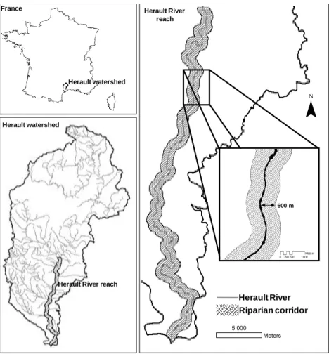
Our research was implemented on the riparian corridor of the downstream reach of the Herault River, located in southern France (Figure 1). It is a 5th _{order river according to the Strahler stream system}

ordination (Strahler, 1952) and the total stream length of the studied reach is 80 km. This part of the Herault watershed comprises an alluvial and a littoral plain. Agriculture, especially vineyards, is the main land use type in this region. Recently, simultaneously with the development of tourism, the fast economic growth of cities has lead to the intensive urbanization of the Herault plain (Balestrat et al., 2008). The riparian corridor width is usually correlated to the width of the river bed. Studies on the Loire watershed (in France) have indicated that it is possible to estimate the average width of river beds from the Strahler stream order (Souchon et al., 2000). Following these results, riparian buffer distances along both sides of the rivers were determined according using a distance of 600 m for the 5th stream order. Data was obtained from the French hydrographic network database, the BDCarthage® produced by the French National Geographic Institute (IGN) from topographic maps (1:50 000) and Spot imagery.

2.2. Land cover pressure typology

A typology of land cover pressure was designed based on a literature review of mechanisms degrading or maintaining stream ecological status (Naiman et al., 2005) and on the recent advances in large scale analysis of the relationships between land cover and stream conditions (Allan, 2004; Hughes et al., 2006). As a result, six thematic classes of interest were defined: “C1-water surfaces”, “C2-agricultural areas”, “C3-urban areas”, “C4-forested areas”, “C5-semi-natural herbaceous vegetation” (meadow and pasture land) and “C6-natural bare soil”.

C1 and C6 categories were defined in order to delineate river water bodies (stream bed and stream banks). C2 and C3 are considered as the two categories causing the main alteration of stream ecological status according to large scale statistical analyses (Allan, 2004). Agricultural practices on land adjacent to streams can lead to soil erosion and subsequent runoff of fine sediments, nutrients, and pesticides (e.g., Cuffney et al., 2000; Schulz and Liess, 1999). Urbanization leads to enhanced runoff, channel erosion, and reduced water quality due to inputs of metals, oils, and road salts (e.g., Booth and Jackson, 1997; Hammer, 1972; Paul and Meyer, 2001). Both land uses degrade the composition and abundance of riparian vegetation.

C4 and C5 are the main types of semi-natural vegetation (wooded and grassy) of the corridor that maintain biodiversity and regulate non-point source pollution (Lyons et al., 2000; Naiman and Decamps, 1997). Wooded vegetation provides stream shading, large woody debris and fine organic matter and both regulates the flux of up-land derived sediments, nutrients and other chemicals and stabilizes stream banks. The forested riparian buffer was widely analysed in large-scale relationship studies and was demonstrated to play an important role on fish and macroinvertebrate communities (Stewart et al., 2001).

Herault watershed

France

Herault watershed

Herault River reach

Herault River reach 5 000 Meters

¯

Figure 1. Study area: the riparian corridor (right) of the downstream reach of the Herault river (bottom left), located in the South of France (top left)

2.3. Data

2.3.1High spatial resolution remotely-sensed data

Considering the spatial extent of riparian areas and the diversity of land cover types within these areas, their study requires multi-source High Spatial Resolution Imagery (HRSI) data (Müller, 1997). Two HSRI data sets available on the whole French territory were chosen.

First, Aerial photographs (5×5 km²) with 0.5 m spatial resolution and spectral information in the visible bands were collected for fine detection of riparian land cover objects. These aerial photographs are orthorectified images (orthophotos) distributed by the French national geographical agency IGN® (Paparoditis et al., 2006). 15 orthophotos acquired in summer 2001 were used to cover the study area. An orthorectified SPOT 5 XS (60 × 60 km²) scene with four spectral bands (B1 to B4) was used in addition to the orthophotos for a more accurate discrimination of vegetation classes and extraction of water body objects (Tormos et al., 2006). Bands B1 (green: 0.50–0.59 μm), B2 (red: 0.61–0.68 μm) and B3 (near infrared: 0.78–0.89 μm) have a spatial resolution of 10 m and band B4 (mid-infrared, 1.58–1.75 μm) has a spatial resolution of 20 m. SPOT 5 XS scenes are orthorectified satellite images, available from SPOT Image©. To cover large geographic areas or specific locations, 10m resolution SPOT 5 XS images are often the most cost effective and efficient solution. For this study we used a SPOT 5 XS archive image acquired on 2004 May 14th.

2.3.2 CORINE Land cover data

The harmonised European land cover database, CORINE Land Cover (CLC), was built by visual interpretation of both Landsat and SPOT satellite images. Interpretation of the images is based on transparencies overlaid on 1/100.000 hard copy prints of satellites images (Bossard et al., 2000). It is based on a standard nomenclature organized into a 3-level hierarchy containing 44 classes. CLC features, characterized by a 25 ha minimum area, are either homogenous areas or combinations of land cover types with a certain recognizable structure. For this study, CLC database was aggregated according to the 6-class land cover pressure typology (see 2.2).

2.4. Land cover classification from HSRI 2.4.1 Image processing

When spatial resolution is increased, image spectral and spatial information becomes highly heterogeneous and conventional pixel-based classification techniques are no longer suitable to classify land cover (Durieux et al., 2008; Ivits and Koch, 2002). Blaschke et al., (2000) suggest as an efficient solution the use of object-based image analysis where, in a first step, homogeneous regions are built up through a segmentation process (segments are also called image objects) and, in a second step, a classification process is applied to these image objects using spectral as well as spatial information such as texture, shape and context features. Such methods improve the discrimination level between spectrally similar land cover types in riparian areas (Goetz et al., 2003).

The software used to implement the method in this study was eCognition4® from Definiens. It provides a complete set of tools for object-based image analysis with a multi-resolution segmentation algorithm (Baatz et al., 2000). The multi-resolution approach, based on a region-growing procedure, was used for land cover classification along the river corridor. A complete description of the region-growing algorithm can be found in (Baatz and Schäpe, 2000) or (Benz et al., 2004). The size and shape of the resulting objects can be empirically determined by the user (Blaschke and Hay, 2001).

Various classification methods (supervised or not) can be used. Their application to image objects offers several advantages compared to pixel-based methods: spectral, textural, contextual, shape and scale information associated to each object can be integrated into the classification hierarchical set of rules, or into the classification feature space for supervised classifications, to improve the quality of classification results (Benz et al., 2004).

In a first step, riparian land cover objects were delineated at a given segmentation level using both aerial photographs and PIR information from the SPOT 5 XS image.

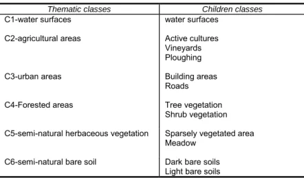
Then, the resulting image objects were classified using a Nearest Neighbour (NN) supervised algorithm in order to discriminate thematic classes according to the land cover pressure typology. The optimal feature space for the nearest neighbour supervised classification method was identified using the Feature Space Optimization (FSO), a classification support tool in the eCognition software. The FSO enabled us to select an optimal set of variables from the range of available spectral, textural, contextual and shape variables, according to patterns expressed in the data set of training objects. The training data set, representing 5 % of all image objects, was visually selected on images. Due to the spectral heterogeneity among training objects of a given thematic class, we had to create new “children classes” (see Table 1) for each thematic class (except for C1) to avoid spectral overlapping. For example, we distinguished two types of “semi-natural bare soil” (C6) because bare soils with two distinct spectral responses exist in the Herault river plain. The class of each training object was identified in the field (May 2005) using the children class nomenclature. Finally, each image object was classified by allocating the children class of the nearest training sample object in the optimal feature space, and the resulting classification was exported in vector format after merging objects according to their land cover class (see 2.2).

Table 1: Hierarchical structure of classes between the 6 thematic classes and the 12 children classes

Thematic classes Children classes

C1-water surfaces water surfaces C2-agricultural areas Active cultures

Vineyards Ploughing C3-urban areas Building areas

Roads C4-Forested areas Tree vegetation

Shrub vegetation C5-semi-natural herbaceous vegetation Sparsely vegetated area

Meadow C6-semi-natural bare soil Dark bare soils

2.4.2 Map validation

The assessment of the accuracy of the resulting land cover map was based on the analysis of a confusion matrix, computed using a set of sampled reference objects (representing 2 % of all image objects) which were visually selected on images and identified on the field (May 2005) according to the land cover pressure typology. The reference objects were different from the training objects and were not used in the classification process. The confusion matrix was built according to pixels contained in the reference objects using Erdas Imagine® software. The accuracy assessment reports three values (Congalton, 1991): (1) the overall accuracy which indicates the proportion of pixels that are correctly classified by the method; (2) the user’s accuracy which is a statistic that indicates to the map user which percentage of a map class actually corresponds to this class and (3) the producer’s accuracy which is a statistic that indicates for each class which percentage of the reality is correctly classified in the map.

2.5. GIS analysis

Two GIS analyses were conducted. A preliminary analysis was performed in order to compare the relevance of information from the CLC- and from the HSRI-derived map (see 2.5.2), before developing the spatial land cover pressure indicators from HSRI-derived map (see 2.5.3). These analyses required specific GIS processing presented in part 2.5.1.

2.5.1 GIS processing

The domain over which spatial indicators are computed at the riparian scale is generally defined by combining a lateral distance to the river with longitudinal distances upstream and downstream from the ecological station where stream ecological status is measured. These distances are often chosen arbitrarily (Frimpong et al., 2005b). However, as no ecological station exists on this part of the Herault River, spatial indicators were computed on 10 sections (A to J) of equal length (8 km). As a result, the GIS analysis focussed on the lateral distance to the river. It was conducted following a three step approach, using ArcGis ® software.

First, the river bed was delineated for a precise delimitation of the lateral distance. For this purpose we selected from the HSRI-derived map all objects classified as “water surfaces” (C6 class) and located near the Herault River hydrographic network (i.e., water object intersected by a 30-m buffer along the hydrographic network). This selection was visually checked on orthophotos and corrected when necessary before merging all polygons in order to construct a uniform polygon representing the Herault River bed.

Then, relevant land cover polygons were selected according to their lateral distance to the river bed, using two techniques: (i) by clipping Land cover data according to the limits of a buffer with a given distance from the river bed polygon (the “buffer technique” - Figure 2A); (ii) by selecting a given type of land cover polygons in contact (having a common border) with the river bed (“the contact technique” - Figure 2 B). While the first technique defines a fixed lateral distance, the second defines a variable one. Depending on the technique employed and the lateral distance chosen for the first technique, the meaning of the spatial indicator is different (see 2.5.3).

Finally, structural attributes of these polygons (e.g. area, perimeter…) were extracted using traditional GIS techniques and specific processing to quantify the width distribution (transversal to the river) of polygons in contact with the river.

2.5.2 Comparison of land cover maps

To compare information from CLC and the HSRI-derived map on the study area, we first computed the confusion matrix for the CLC map, using the same sample of reference objects as for the HSRI map (see 2.4.2) (comparison of accuracy between the two maps). Then, we analysed the land cover composition (area percentage of each land cover class) according to different buffer widths (lateral distances) along the whole Herault River reach (80 Km). Two ranges of lateral distances were defined. The first range aims to analyse pressure characteristics in the immediate proximity of the river (5, 10, 15, 20, 25, 30, 35, 40, 45 and 50 meters). The second range concerns the vicinity of the river (100, 150, 200, 250, 300, 350, 400, 450, and 500 meters). The lateral distance was delimited using the buffer technique (see Figure 2A).

A

B

¯

Figure 2. Presentation of the two GIS techniques for the extraction of relevant polygons according to a lateral distance to the river bed. In figure 2A, the “buffer technique” : first a buffer is computed along the river bed according to a given distance and then land cover polygons are clipped into the buffer limits. In Figure 2B, the “contact technique” : all polygons of a given land cover type in contact (having a common border) with the river bed are selected.

2.5.3 Spatial indicators of land cover pressure

Six spatial indicators characterizing the river corridor land cover where used as potential measurements of pressure on the stream ecological status. Spatial indicators were developed for each section of Herault River main reach (10 section from A to J of equal length). Table 2 summarizes indicator characteristics and the GIS processing used to construct them (see 3.3.1).

The first three spatial indicators are of the “area percentage” type. They focus on the proportion of a given land cover type along the river corridor in the delimited area: the Linear Spatial Indicator (LSI), the Floodplain Spatial Indicator (FSI), and the Contact Spatial Indicator (CSI). Area percentages, indicating the presence and intensity of land cover pressure are the main landscape structure attributes used at the riparian scale in studies of large scale relationships and remain the main explanatory land cover variable of stream condition. While the LSI represents the presence and intensity of pressure on a buffer close to the stream (10 m width), the FSI quantifies it on the whole river corridor (600 m width). In contrast the CSI is not restrained to a buffer and deals with pressure polygons directly in contact with the river.

Three additional indicators were designed to characterize the forested component of the riparian buffer more specifically. In many streams, the presence of forested riparian buffer strips can efficiently reduce groundwater nitrogen loads and surface runoff phosphorus loads (Naiman and Decamps, 1997). Furthermore, the spatial patterns of forested riparian zones may influence their ability to act as nutrient sinks. Thus indicators that characterize the spatial pattern of forested riparian areas can be useful. A simple model of an upland contributing area and a forested riparian buffer by Weller et al., (1998) explored the relationship between the spatial configuration and nutrient retention capacity of riparian zones. According to the results of this heuristic model, we defined: (i) the Average Forested Riparian zone Width (AFRW) which quantifies approximately the average buffer width of forested riparian strips, and is the best predictor of lateral runoff for non-retentive buffers; (ii) the Forested Riparian zone Uniformity (FRU) which indicates the variability (the uniformity) of this forested buffer width. Irregular buffer widths are less efficient than uniform buffer widths because transfer through gaps dominates lateral runoff; (iii) the Forested Riparian zone Continuity (FRC) which indicates the frequency of gaps (the fragmentation or discontinuity) of the forested riparian strip and is the best predictor of lateral runoff for narrow, retentive buffers.

Table 2: Characteristics of the six spatial indicators developed in this study

3. Results and discussion

3.1 Land cover classification from HSRI

Table 3 shows the error matrix, overall accuracy and both user’s and producer’s accuracies of the HSRI derived land cover classification. The error matrix is expressed in number of pixels. Lines represent classes in reality; while columns represent classes on the map: each pixel thus appears in one cell. Overall accuracy was 70%. All “C1-water surfaces” objects were correctly classified. Accurate results were obtained for “C2-agricultural areas” and “C4-forested areas” too (user’s and producer's accuracies are 88% and 73%, and 74% and 64%, respectively). “C3-urban areas” presents a lower accuracy (user’s and producer's accuracy are 46% and 57% respectively). The accuracy of the map obtained with the object-based method is poor for both “C5-semi-natural herbaceous vegetation” and “C6-semi-natural bare soils” classes (user’s and producer's accuracies are 27% and 37%, and 9% and 40%, respectively).

In the case of the C5 class, both commission and omission errors were encountered especially with “C2-agricultural areas”. Confusion between these two classes is probably due to the fact that the SPOT 5 image was acquired during the spring season, at a time of year when some crops (e.g. wheat, barley) show a spectral behaviour similar to semi-natural grass cover. Using satellite images acquired during the summer season may help to avoid spectral confusion between these classes. Grassy or herbaceous vegetation in riparian corridors can have a beneficial impact on stream status and may be appropriate restoration options in some situations, especially in agricultural regions (Lyons et al., 2000). Therefore, proper identification of this class is of major importance. For the C6 class, the low accuracy originates from strong confusions with “C2-agricultural areas” and “C3-urban areas”. Spectral behaviour of bare soils can be similar to that of ploughings, vineyards and house roofs (tile cover). The use of specific textural attributes could improve the discrimination between these classes, thus leading to an increased accuracy. Furthermore, the lagtime between remotely sensed image acquisition (May 2004 for SPOT 5 XS image and summer 2001 for orthophotos) and reference data set acquisition (May 2005) can also explain part of the misclassifications.

In the perspective of large scale mapping of land cover along river corridors, classification methods have to be cost-effective and easy to reproduce in distinct areas. However, implementation of the Nearest Neighbour (NN) technique on the Herault River reach was very time-consuming for the definition and the in situ acquisition of training sample objects and the classification rules automatically inferred by the FSO (see 2.4.1.) were hard to understand and to refine.

Consequently, the NN method seems to be unsuitable for large scale mapping. On the contrary, rule-based classification appears more adapted. In this approach, a logical decision tree is built based on feature space and physical features of each class that can be applied in other places. It allows easy integration of remotely sensed data with other sources of geo-referenced information, such as land use data and spatial texture, to obtain higher classification accuracy, especially for herbaceous vegetation. All rules can be refined with full user control, at any time in the classification process and, in most cases, without changing the class allocation of other objects (Lucas et al., 2007). This was implemented on the study area and on the overall Herault River hydrographic network (1500 km long), but is not presented here.

Table 3: Error matrix and accuracy values of riparian land cover classification from HSRI (in number of pixels, 0.5 m pixel size)

Table 4: Error matrix and accuracy values of the CORINE land cover map (in number of pixels, 0.5 m pixel size)

3.2 Comparison of land cover maps

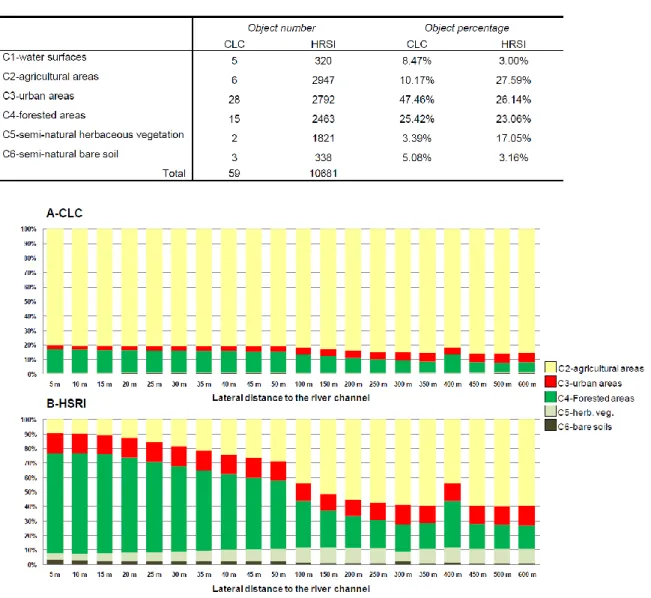
When comparing the number of polygons (objects) for each land cover type between CORINE Land Cover (CLC) and the HSRI-derived map (see table 5 and figure 8), it clearly appears that, due to its finer spatial resolution, the HSRI map provides much more information than the CLC database. For example, only 15 polygons of “C4-forested areas” are detected with the CLC database against 2463 with the HSRI-derived map, which means that the CLC resolution is much too low to detect the heterogeneity of forested areas in riparian areas. Furthermore the different classes in the CLC map appear not to be aggregated in the same way: C2 Agricultural areas appears to be strongly aggregated (10% of objects in CLC against 28% in HSRI) while C3 Urban areas is under aggregated (47% in CLC against 26% in HSRI). This will have an impact on spatial indicators that depends on the relative number of objects.

Table 4 shows the error matrix, overall accuracy and both user’s and producer’s accuracies of the CLC map. Overall accuracy was 54%. “C5-semi-natural herbaceous vegetation” and “C6-semi-natural bare soils” reference objects were not detected by CLC (no pixel in the confusion matrix) and all “C1 -water surfaces” objects were incorrectly classified (both user’s and producer's accuracies were 0%). Highest accuracy results were obtained for “C2-agricultural areas” and “C3-urban areas” (user’s and producer's accuracies were 59% and 96%, and 77% and 26%, respectively). “C4-forested areas” presented a lower accuracy (user’s and producer's accuracy were 36% and 33% respectively).

Accuracy results of the CLC map are lower than those of the HSRI-derived map and confirm the limits of coarse land cover data for the accurate mapping of land cover along a river corridor. The “C4-forested areas” class is poorly characterized by the CLC map due to the strong confusion with “C1-water surfaces” and “C2-agricultural areas”. Although a high percentage of the “C3-urban areas” class from CLC corresponds to the reality, a low percentage of C3 reference objects is detected by CLC. On the contrary, because of the predominance of the “C2-agricultural areas” class along the riparian

corridor of the Herault River, the majority of C2 reference objects are correctly detected (96%) by CLC, while only 59% of CLC C2 objects actually correspond to the reality.

In Figure 3, the evolution of the land cover composition (Area Percentage indicator) according to the lateral distance from the Herault River (buffer width from 5m to 600 m) shows that major landscape patterns inside the riparian area which are revealed by HSRI maps, are totally smoothed in CLC maps. In the case of CLC (Figure 2A), spatial information does not significantly change with the buffer width whatever the land cover class. The “C2-agricultural areas” class is predominant both at the contact and in the vicinity of the river. In contrast, the HSRI-derived map (Figure 2B) highlights a spatial change in the land cover structure according to the lateral distance from the river channel, especially for “C4-forested areas” and “C2-agricultural areas” classes. Near the river (between 5 and 50 meters on both sides of the river) C4 is predominant, while C2 is dominant for riparian buffer zones larger than 100m. Such results prove that the CLC database is, as expected, less accurate than the HSRI-derived map, and that the differences between the maps decrease as buffer width increases (up to 150 m). This is of major importance regarding linear corridors whose structure cannot be correctly described by CLC data. Similar results have been presented in the literature (Lattin et al., 2004; Shuft et al., 1999). It is most likely that, in many situations within river corridors, the generalisation level of the CLC database will lead to under- or overestimation of the effect of cover types which impact on stream chemical and biotic metrics (Goetz, 2006). This work clearly demonstrates the interest of HSRI information for improving the quantification of land cover amount and arrangement patterns at the riparian scale.

Table 5: Comparison of the number of objects for each land cover type for both CORINE Land Cover (CLC) and High Spatial Resolution Imagery (HSRI)-derived maps

Figure 3. Variation of the area percentage of a given land cover type according to the lateral distance to the river channel on the Herault river reach. (A) from CORINE Land Cover (CLC) database, (B) from the High Spatial Resolution Imagery (HSRI)-derived map

3.3 Spatial indicators of land cover pressures

Figures 4 to 7 show results of synthetic spatial indicators computed from both land cover maps (CLC and HSRI) for the 10 sections of the Herault River reach.

First, information given by each spatial indicator differs according to the land cover data used (CLC or HSRI) except for the Floodplain Spatial Indicator (FSI). For instance, the Linear Spatial Indicator (LSI) is significantly different for the two land cover maps: while “C4-forested areas” is predominant with the HSRI land cover map, “C2-agricultural areas” is dominant with the CLC database on most of the sections. In contrast, the FSI shows a predominance of agricultural areas (C2) for both sets of land cover data. These results confirm the occurrence of large differences from both land cover data, which get blurred with higher buffer widths. Furthermore, when forest areas (C4) are detected in contact with the river using the CLC database, we observe that cover areas are consistently overestimated: the value of the Average of Forest Riparian Width (AFRW) indicator extracted from the CLC database is always overvalued compared to the HSRI map. Figure 8 compares maps from both land cover data sets on a fraction of section D. The overestimation of the forested riparian strip by CLC is obvious, while the HSRI map better agrees with reality.

The analysis of HSRI-derived indicators on river sections gives interesting and complementary information on the presence and the intensity of pressure and on the characteristics of the forested riparian strip along the Herault River reach.

The LSI (Figure 4B) indicates a high presence of forested areas (C4) on the riparian strip close to the stream for all sections except for section J which is dominated by urban areas due to the presence of Agde city at the river mouth.

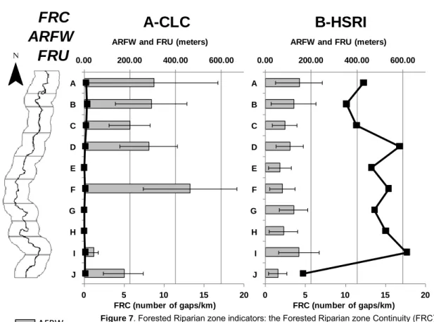
In addition, the CSI (Figure 6B) specifies the intensity of pressure bordering the stream. Although the CSI confirms the impact of urban land cover on section J and the presence of a forested riparian strip on the other ones, it also reveals and quantifies the existence of gaps along this forested band. Sections D, E, F, G, and I are potentially affected by nutrient, sediment, and pollutant fluxes from agricultural plots in direct contact with the river. Figure 7B shows indicators related to attributes of the forested riparian strip and the occurrence of gaps in each of the sections is highlighted by the Forested Riparian zone Continuity (FRC) indicator.

The nitrogen retention capacity of the riparian buffer zone could be assessed using both the Average Forested Riparian zone Width (AFRW) and the Forested Riparian zone Uniformity (FRU). A, G and I sections are characterized by a wide forested riparian strip along the river (AFRW is 148 m, 125 m and 147 m, respectively) but this strip is more uniform on G (FRU is 63) than on A and I (FRU is 102 m and 89 m, respectively).

Although many other factors (e.g. climate, topography, land use, stream type and structure, slope, soil type, and drainage characteristics) influence (i) the volume of sediment and agricultural chemicals reaching the stream network and (ii) the riparian functions (Naiman et al., 2005), this set of indicators is liable to provide explanatory variables for assessing stream ecological status. The detailed land cover map provides considerable flexibility for the calculation of various structure attributes of land cover pressure and riparian vegetation along rivers. However, the error in land cover classification will have to be analysed in detail to associate uncertainty values to these indicators (Gergel et al., 2007).

Based on this approach some properties of the river corridor can be examined more precisely, like for instance the continuity (connectivity) of the forested riparian strip, considered as a key attribute in assessing riparian functions (Naiman and Decamps, 1997). Additionally to the number of gaps (FRC), the longitudinal extent, mean length, and maximum length of gaps could be assessed. Such complementary information highlights properties of riparian connectivity. Indeed, while a number of short gaps in the forested riparian strip may have little effect on stream temperature, they may be significant channels for direct transport to the stream of upland nutrients, sediments and pollutants (Naiman and Decamps, 1997). On the other hand, large gaps in forested vegetation, approaching one kilometre in length, have been demonstrated to have significant effects on stream temperature and trout distribution (Barton et al., 1985).

A-CLC

B-HSRI

LSI

Figure 4. Linear Spatial Indicator (LSI): the surface area percentage of a given land cover category extracted on a 10-meter buffer. In A from CORINE Land Cover (CLC) database, in B from the High Spatial Resolution Imagery (HSRI)-derived map

A-CLC

B-HSRI

FSI

Figure 5. Floodplain Spatial Indicator (FSI): the surface area percentage of a given land cover category extracted on a 600-meter buffer. In A from CORINE Land Cover (CLC) database, in B from the High Spatial Resolution Imagery (HSRI)-derived map

A-CLC

B-HSRI

CSI

Figure 6. Contact Spatial Indicator (CSI): the surface area percentage of a given land cover category in contact with the river channel. In A from CORINE Land Cover (CLC) database, in B from the High Spatial Resolution Imagery (HSRI)-derived map

0 5 10 15 20 0.00 200.00 400.00 600.00 A B C D E F G H I J 0 5 10 15 20 0.00 200.00 400.00 600.00 A B C D E F G H I J

A-CLC

B-HSRI

ARFW

FRU

¯

FRC (number of gaps/km) ARFW and FRU (meters)

FRC (number of gaps/km)

FRC

Figure 7. Forested Riparian zone indicators: the Forested Riparian zone Continuity (FRC): the number of forested areas patches/km in contact with the river; the Average Forested Riparian zone Width (AFRW): the average of the forested riparian strip width (in meters); and the Forested Riparian zone Uniformity (FRU): the variability (standard deviation) of the forested riparian strip width (in meters). In A from CORINE Land Cover (CLC) database, in B from the High Spatial Resolution Imagery (HSRI)-derived map

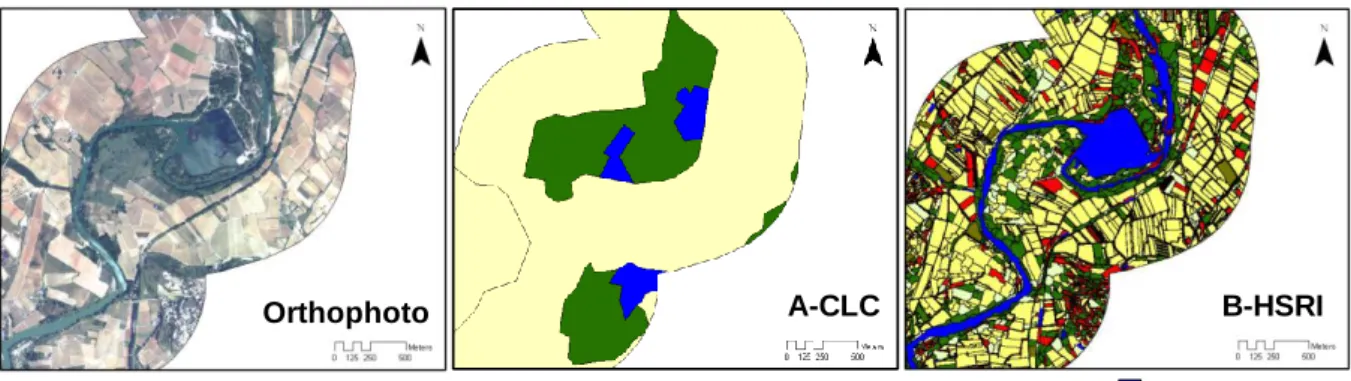
B-HSRI A-CLC

Orthophoto

Figure 8. Comparison with the orthophoto on a part of the section D of the results in A from CORINE Land Cover (CLC) and in B from the High Spatial Resolution Imagery (HSRI)-derived map. Note the overestimation of forested areas that affects riparian vegetation strip indicators

C2-agricultural areas C3-urban areas C4-Forested areas C5-herb. veg. C6-bare soils C1-Water surfaces

4. Summary and conclusion

This study, based on an implementation on the Herault River, has demonstrated that High Spatial Resolution Imagery (HSRI) using object-based image analysis allows the extraction of land cover information along the river corridor with an acceptable degree of confidence (70 % of pixels well classified according to ground reference data), showing far more accuracy and detail than CLC data (54 % of pixels well classified according to ground reference data). The comparison of land cover information and spatial indicators computed from the CORINE Land Cover (CLC) database and from the HSRI-derived map attests that CLC is too coarse to quantify land cover pressure and riparian vegetation properties near the stream (along a 150 m wide strip) in a relevant way. Spatial indicators derived from the HSRI map provide accurate and original information on the presence and intensity of pressure close to the stream and on forested riparian strip attributes (uniformity, mean width and continuity). Detailed land cover data introduced in GIS allows large flexibility and reliability for the calculation of spatial indicators, which aim to characterize the mechanisms through which land cover along river corridors impacts stream ecosystems.

Given these results, new challenges have emerged in view of gaining a better understanding of the relationships between land cover pressure and stream ecological status.

The first challenge consists in the development of a rule-based object oriented classification method for large scale mapping of land cover along river corridors using HSRI. Because supervised classification techniques (such as nearest neighbour used in this study) are strongly dependent on the training sample which is time-consuming to define and collect, we argue that rule-based classification would be more a more efficient technique to map land cover on large territories.

The second challenge consists in (i) the definition of a set of complementary spatial indicators related to the riparian functions and to the mechanisms of land cover pressure on a given stream condition (chemical, physical or biotic) and (ii) the development of GIS techniques to define these indicators automatically. Sensitivity of these spatial indicators to the error in land cover classification will have to be analysed in detail and resulting uncertainty values will be associated to these indicators.

Finally, the last challenge consists in the study and modelling of the ecological (or chemical) response to spatial indicators derived from the HSRI map and other pressure variables, in order to identify the minimum width and composition of riparian vegetation that should be recommended on a regional or national scale to maintain river corridor functions for stream integrity and ecological status.

Acknowledgment

This study has been made possible by a PhD grant from the French Ministry of Research. The work has been partly realised in the framework of a research contract between ONEMA and Cemagref. Acquisition of remote sensing data benefited from the support of the ISIS programme of the French national space agency CNES (Spot5 images), while IGN airborne orthophotos were made available by the French Ministry of Agriculture.

References

Allan, J.D., 2004. Landscapes and Riverscapes: The Influence of Land Use on Stream Ecosystems. Annual Review of Ecology, Evolution, and Systematics 35 (2004), pp. 257-284.

Allan, J.D., Erickson, D., Fay, J., 1997. The influence of catchment land use on stream integrity across multiple spatial scales. Freshwater Biology 37 (1997), pp. 149-161.

Baatz, M., Heynen, M., Hofmann, P., Lingenfelder, I., Mimler, M., Schäpe, A., Weber, M., Willhauck, G., 2000. eCognition User Guide. Definiens AG, München, p. 483.

Baatz, M., Schäpe, A., 2000. Multiresolution Segmentation – an optimization approach for high quality multi-scale image segmentation. Angewandte Geographische Informationsverarbeitung 12 (2000), pp. 12-23.

Balestrat, M., Chéry, J.-P., Valette, E., 2008. Suivi des changements d’occupation et d’utilisation du sol pour la compréhension des dynamiques périurbaines, XLV colloque de l’Association Régionale de Langue Française, Rimouski (Québec).

Barton, D.R., Taylor, W.D., Biette, R.M., 1985. Dimension of riparian buffer strips required to maintain trout habitat in southern Ontario streams. North American Journal of Fisheries Management 5 (1985), pp. 364-378.

Benz, U.C., Hofmann, P., Willhauck, G., Lingenfelder, I., Heynen, M., 2004. Multi-resolution, object-oriented fuzzy analysis of remote sensing data for GIS-ready information. ISPRS Journal of Photogrammetry and Remote Sensing 58 (2004), pp. 239-258.

Blaschke, T., Hay, G.J., 2001. Object-oriented Image Analysis and Scale-space: Theory and Methods for Modeling and Evaluating Multiscale Landscape Structures. International Archives of Photogrammetry and Remote Sensing 34 (2001), pp. 22-29.

Blaschke, T., Lang, S., Lorup, E., Strobl, J., Zeil, P., 2000. Object-oriented image processing in an integrated GIS/remote sensing environment and perspectives for environmental applications. Umweltinformation Für Planung, Politik und Öffentlichkeit / Environmental Information for Planning, Politics and the Public 2 (2000), pp. 555-570.

Booth, D.B., Jackson, C.R., 1997. Urbanization of aquatic systems: Degradation thresholds, stormwater detection, and the limits of mitigation. Journal of the American Water Resources Association 33 (1997), pp. 1077-1090.

Bossard, M., Feranec, J., Otahel, J., 2000. CORINE land cover technical guide-Addeendum 2000, Technical report No 40. European Environment Agency.

Congalton, R.G., 1991. A review of assessing the accuracy of classifications of remotely sensed data. Remote sensing of environment 37 (1991), pp. 35-46.

Cuffney, T.F., Meador, M.R., Porter, S.D., Gurtz, M.E., 2000. Responses of physical, chemical, and biological indicators of water quality to a gradient of agricultural land use in the Yakima River Basin, Washington. Environmental Monitoring and Assessment 64 (2000), pp. 259-270.

Durieux, L., Lagabrielle, E., Nelson, A., 2008. A method for monitoring building construction in urban sprawl areas using object-based analysis of Spot 5 images and existing GIS data. ISPRS Journal of Photogrammetry and Remote Sensing 63 (2008), pp. 399-408.

Frimpong, E.A., Sutton, T.M., Lim, K.J., Hrodey, P.J., Engel, B.A., Simon, T.P., Lee, J.G., Le Master, D.C., 2005a. Determination of optimal riparian forest buffer dimensions for stream biota- landscape association models using multimetric and multivariate responses. Canadian Journal of Fisheries and Aquatic Sciences 62 (2005a), pp. 1-6.

Frimpong, E.A., Sutton, T.M., Lim, K.J., Hrodey, P.J., Engel, B.A., Simon, T.P., Lee, J.G., Le Master, D.C., 2005b. Determination of optimal riparian forest buffer dimensions for stream biota landscape association models using multimetric and multivariate responses. Canadian Journal of Fisheries and Aquatic Sciences 62 (2005b), pp. 1-6.

Gergel, S.E., Stange, Y., Coops, N.C., Johansen, K., Kirby, K.R., 2007. What is the value of a good map? An example using high spatial resolution imagery to aid riparian restoration. Ecosystems 10 (2007), pp. 688-702.

Gergel, S.E., Turner, M.G., Miller, J.R., Melack, J.M., Stanley, E.H., 2002. Landscape indicators of human impacts to riverine systems. Aquatic Sciences 34 (2002), pp. 118-128.

Goetz, S.J., 2006. Remote sensing of riparian buffers: Past progress and future prospects. Journal of the American Water Resources Association 42 (2006), pp. 133-143.

Goetz, S.J., Wright, R., Smith, A.J., Zinecker, E., Schaub, E., 2003. Ikonos imagery for resource management: Tree cover, impervious surfaces and riparian buffer analyses in the mid-Atlantic region. Remote sensing of environment 88 (2003), pp. 195-208.

Gregory, S.V., Swanson, F.J., McKee, W.A., Cummins, K.W., 1991. An ecosystem perspective of riparian zones. BioScience 41 (1991), pp. 540-551.

Hammer, T.R., 1972. Stream Channel Enlargement Due to Urbanization Water Resource Research 8 (1972), pp. 1530–1540.

Hughes, R.M., Wang, L., Seelbach, P.W., 2006. Landscapes influences on Stream Habitats and Biological Assemblages. American Fisheries Society, Bethesda, Maryland.

Ivits, E., Koch, B., 2002. Object-Oriented Remote Sensing Tools for Biodiversity Assessment: a European Approach, In: Geoinformation for European-wide Integration.Proceedings of the 22nd EARSeL Symposium, June 4-6, 2002, Prague, Czech Republic. Millpress Science, Netherlands. Johansen, K., Phinn, S., Lowry, J., Douglas, M., 2008. Quantifying indicators of riparian condition in Australian tropical savannas: integrating high spatial resolution imagery and field survey data. International Journal of Remote Sensing 29 (2008), pp. 7003 - 7028.

Jones, K.B., Neale, A.C., Nash, M.S., Van Remortel, R.D., Wickham, J.D., Riitters, K.H., O'Neill, R.V., 2001. Predicting nutrient and sediment loadings to streams from landscape metrics: A multiple watershed study from the United States Mid-Atlantic Region. Landscape Ecology 16 (2001), pp. 301-312.

Lattin, P., Wiginton, P., Moser, T.J., Peniston, B.E., Lindeman, D.R., Oetter, D.R., 2004. Influence of remote sensing imagery source on quantification of riparian land cover/land use. Journal of the American Water Resources Association 40 (2004), pp. 215-227.

Li, H., Reynolds, J.F., 1995. On definition and quantification of heterogeneity. Oikos 73 (1995), pp. 280-284.

Lucas, R., Rowlands, A., Brown, A., Keyworth, S., Bunting, P., 2007. Rule-based classification of multi-temporal satellite imagery for habitat and agricultural land cover mapping. IJRS International Journal of Photogrammetry and Remote Sensing 62 (2007), pp. 165-185.

Lyons, J., Trimble, S.W., Paine, L.K., 2000. Grass versus trees: Managing riparian areas to benefit streams of central North America. Journal of the American Water Resources Association 36 (2000), pp. 919-930.

Müller, E., 1997. Mapping riparian vegetation along rivers: old concepts and new methods. Aquatic Botany 58 (1997), pp. 437.

Naiman, R.J., Decamps, H., 1997. The ecology of interfaces: Riparian Zones. Annual Review of Ecology and Systematics 28 (1997), pp. 621-658.

Naiman, R.J., Décamps, H., McClain, M.E., 2005. Riparia : ecology, conservation, and management of streamside communities. Elsevier Academic, ©2005, Amsterdam; Boston

Paparoditis, N., Souchon, J.P., Martinoty, G., Pierrot-Deseilligny, M., 2006. High-end aerial digital cameras and their impact on the automation and quality of the production workflow. ISPRS Journal of Photogrammetry and Remote Sensing 60 (2006), pp. 400-412.

Paul, M.J., Meyer, J.L., 2001. Streams in the urban landscape. Annual Review of Ecology and Systematics 32 (2001), pp. 333-365.

Schulz, R., Liess, M., 1999. A field study of the effects of agriculturally derived insecticide input on stream macroinvertebrate dynamics. Aquatic Toxicology 46 (1999), pp. 155-176.

Shuft, M.J., Moser, T.J., Wigington Jr, P.J., Stevens Jr, D.L., McAllister, L.S., Chapman, S., Ernst, T.L., 1999. Development of landscape metrics for characterizing riparian-stream networks. PE&RS - Photogrammetric Engineering and Remote Sensing 65 (1999), pp. 1157-1167.

Souchon, Y., Andriamahefa, H., Cohen, P., Breil, P., Pella, H., Lamouroux, N., Malavoi, J.-R., Wasson, J.-G., 2000. Régionalisation de l'habitat aquatique dans le bassin de la Loire, Synthése. Cemagref Lyon BEA/LHQ, Agence de l'eau Loire Bretagne, p. 291.

Stewart, J.S., Wang, L., Lyons, J., Horwatich, J.A., Bannerman, R., 2001. Influences of watershed, riparian-corridor, and reach-scale characteristics on aquatic biota in agricultural watersheds. Journal of the American Water Resources Association 37 (2001), pp. 1475-1487.

Strahler, A.N., 1952. Hypsometric (area-altitude) analysis of erosional topography. Bulletin Geological Society of America 63 (1952), pp. 1117-1142.

Strayer, D.L., Beighley, R.E., Thompson, L.C., Brooks, S., Nilsson, C., Pinay, G., Naiman, R.J., 2003. Effects of land cover on stream ecosystems: roles of empiricals models and scaling issues. Ecosystems 6 (2003), pp. 407-423.

Tormos, T., Kosuth, P., Durrieu, S., Wasson, J.G., Pella, H., Villeneuve, B., Perez Correa, M., 2006. Use of Multi-Platform-sensing for characterisation of land use in river corridors International Society for Photogrammetric and Remote Sensing-Commission 1 symposium, Paris.

Townsend, C.R., Dolédec, S., Norris, R., Peacock, K., Arbuckle, C., 2003. The influence of scale and geography on relationships between stream community composition and landscape variables: Description and prediction. Freshwater Biology 48 (2003), pp. 768-785.

Turner, M.G., 1989. Landscape ecology: the effect of pattern on process. Annual review of ecology and systematics. Vol. 20 (1989), pp. 171-197.

Weller, D.E., Jordan, T.E., Correll, D.L., 1998. Heuristic models for material discharge from landscapes with riparian buffers. Ecological Applications 8 (1998), pp. 1156-1169.