Computation of the topographic index on 16 watersheds in Quebec.

WATERSHEDS IN QUEBEC

Final report

Agriculture and Agri-Food Canada

Prepared by :

Alain N. Rousseau

Achraf Hentati

Sébastien Tremblay

Renaud Quilbé

Jean -Pierre Villeneuve

Centre Eau, Terre et Environnement

Institut national de la recherche scientifique (INRS-ETE)

490, rue de la Couronne, Québec (QC), G1K 9A9

Report N° R800-f

LIST OF FIGURES ... V LIST OF TABLES ... XI LIST OF ACRONYMS ... XIII

1 INTRODUCTION ... 1

2 REVIEW OF SOME COMPUTATIONAL ALGORITHMS ... 3

2.1 TOPOGRAPHIC INDEX (TI) ... 3

2.1.1 Definition ... 3

2.1.2 Computation of the topographie index ... 5

2.2 PRESENTATION OF THE FLOW DIRECTION ALGORITHMS ... 6

2.2.1 Definition ... 6

2.2.2 Single Flow Direction algorithm (SFD) ... 6

2.2.3 Bülow Direction algorithm (BFD) ... 7

2.2.4 Multiple Flow Direction algorithm (MFD) ... 11

2.3 DISCUSSION ... 11

2.4 CONCLUSION ... 14

3 APPLICATION OF THE ALGORITHMS ON 16 WATERSHEDS ... 15

3.1 TECHNICAL PROCEDURE ... : ... 15

3.1.1 Preparation of the DEM ... 15

3.1.2 Calculation of TI using the D8 algorithm (O'Callaghan and Mark, 1984) ... 16

3.1.4 Calculation of TI using the D8-LAD algorithm (Tarhoton et al., 1997) ... 17

3.2 RESULTS AND DISCUSSIONS ... 18

3.3 RECOMlVIENDATIONS ... 24

4 CONCLUSION ... 25

5 REFERENCES ... 27

APPENDIX A RESULTS OF

TI

DISTRIBUTION ON THE 16 WATERSHEDS ... 29

Figure 2.1 : Saturation excess overland flow ... 3

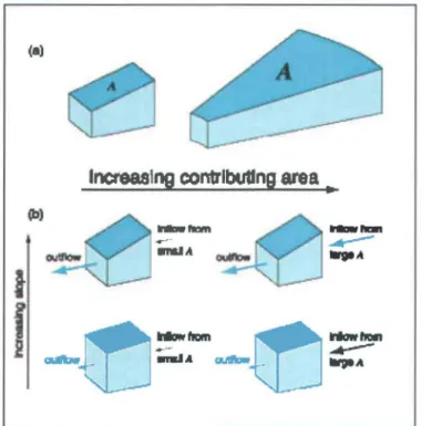
Figure 2.2: Influence of local slope and contributing area on the water balance of a catchment "block". The inflow rate is proportional to the contributing area A (a) and the outflow rate is controlled by the local slope (b) [Hornberger et al., 1998] ... 4

Figure 2.3 : High values of TI are in valleys and low values are at tops of hillslopes [farboton, 2003] ... 5

Figure 2.4: The upslope contributing area and the contour length ... 6

Figure 2.5 : Eight flow direction method (D8) ... 7

Figure 2.6: Flow directions defmed as steepest downward slope on planar triangular facets on a block centered grid [farboton, 1997] ... 8

Figure 2.7 : Definition of variable for the calculation of slope on a single triangular facet [farboton, 1997] ... 8

Figure 2.8: The elementary computational used in the D8-LAD and the D8-LTD methods [Orlandini et al., 2003] ... 10

Figure 2.9: Weights attributed to flow directions in the MFD of Quinn etaI., [1991]. ... 11

Figure 2.10: The "burning" process ... 13

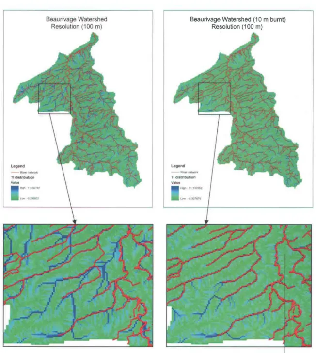
Figure 3.1 : Comparison of TI distributions obtained by the D8 method on the Beaurivage watershed (100 m grid resolution) without the 'burning' process (left) and with the 'burning' process (right) ... 21

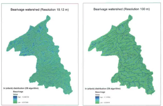
Figure 3.2 : TI distributions obtained by the D8 method on the Beaurivage watershed for the two grid resolutions (19.12 m and 100 m) ... 22

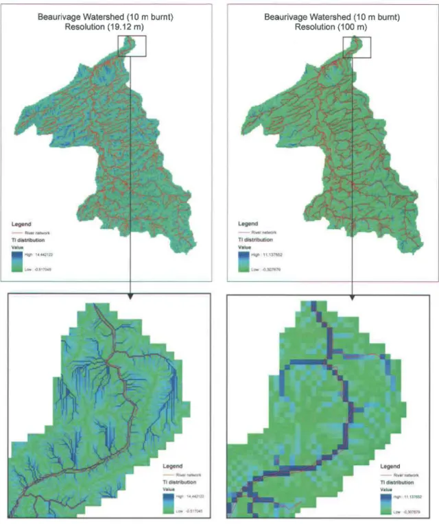
Figure 3.3 : The resolution effect (19 m and 100 m) on TI distributions obtained by the D8 method on the Beaurivage watershed ... 23

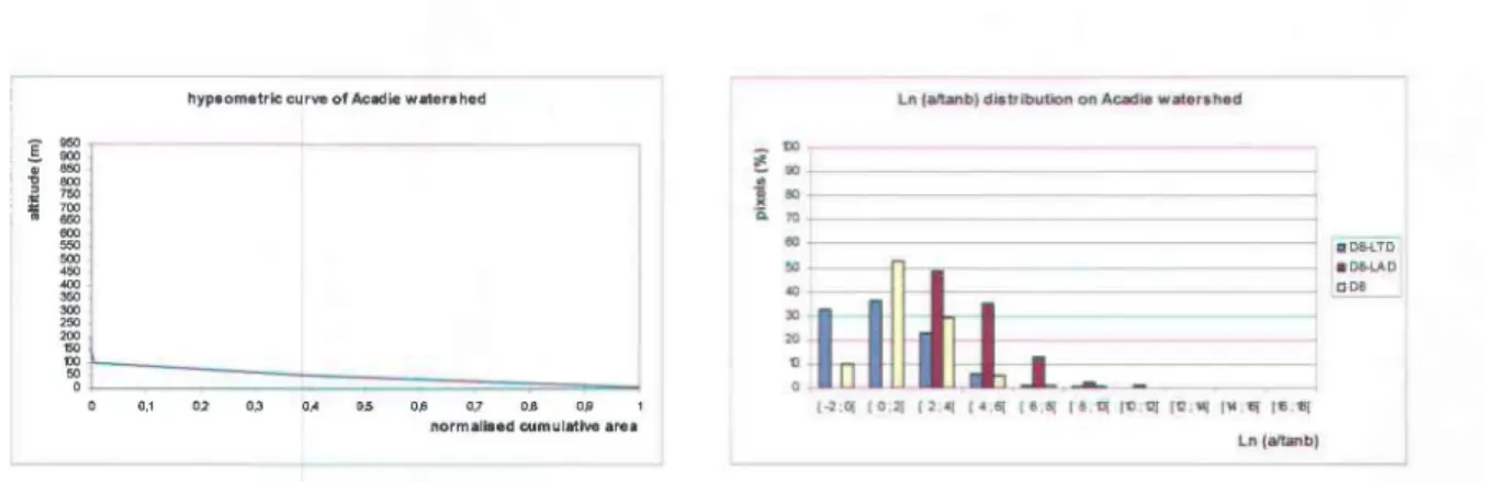
Figure A.l : Hypsometric curve and TI distributions on Acadie river watershed obtained by the 3 flow direction algorithms ... 30

Figure A.2 Hypsometric curve and TI distributions on Achigan river watershed obtained by the 3 flow direction algorithms ... 30

Figure A.3 : Hypsometric curve and TI distributions on Des Anglais river watershed obtained by the 3 flow direction algorithms ... 30

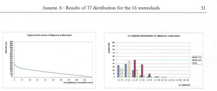
Figure A.4 Hypsometric curve and TI distributions on Bayonne river watershed obtained by the 3 flow direction algorithms ... 31

Figure A.S Hypsometric curve and TI distributions on Beaurivage river watershed obtained by the 3 flow direction algorithms ... 31

Figure A.6 : Hypsometric curve and TI distributions on Boyer river watershed obtained by the 3 flow direction algorithms ... 31

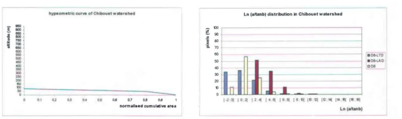
Figure A.7 Hypsometric curve and TI distributions on Chibouet river watershed obtained by the 3 flow direction algorithms ... 32

Figure A.S Hypsometric curve and TI distributions on Coaticook river watershed obtained by the 3 flow direction algorithms ... 32

Figure A.9 : Hypsometric curve and TI distributions on Des Hurons river watershed obtained by the 3 flow direction algorithms ... 32

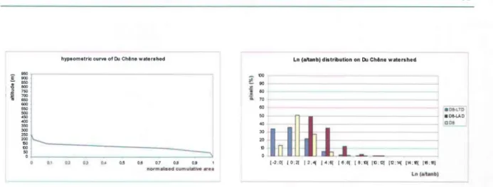
Figure A.l0 Hypsometric curve and TI distributions on Du Chêne river watershed obtained by the 3 flow direction algorithms ... 33

Figure A.ll Hypsometric curve and TI distributions on Etchemin river watershed obtained by the 3 flow direction algorithms ... 33

Figure A.12 Hypsometric curve and TI distributions on Mascouche river watershed obtained by the 3 flow direction algorithms ... 33

Figure A.13 : Hypsometric curve and TI distributions on Nicolet river watershed obtained by the 3 flow direction algorithms ... 34

Figure A.14 : Hypsometric curve and TI distributions on Noire river watershed obtained by the 3 flow direction algorithms ... 34

Figure A.15 : Hypsometric curve and TI distributions on Saint-Esprit river watershed obtained by the 3 flow direction algorithms ... 34

Figure A.16 Hypsometric curve and TI distributions on Yamaska river watershed obtained by the 3 flow direction algorithms ... 35

Figure A.17 TI results for the Acadie river watershed using the D8 algorithm (Arc Hydro tool) ... 36

Figure A.18 : TI results for the Achigan river watershed using the D8 algorithm (Arc Hydro tool) ... 37

Figure A.19 TI results for the Anglais river watershed using the D8 algorithm (Arc H ydro tool) ... 38

Figure A.20 : TI results for the Bayonne river watershed using the D8 algorithm (Arc Hydro tool) ... 39

Figure A.21 : TI results for the Beaurivage river watershed using the D8 algorithm (Arc H ydro tool) ... 40

Figure A.22 : TI results for the Boyer river watershed using the D8 algorithm (Arc Hydro tool) ... ... 41

Figure A.23 : TI results for the Chibouet river watershed using the D8 algorithm (Arc Hydro tool) ... 42

Figure A.24 : TI results for the Coaticook river watershed using the D8 algorithm (Arc Hydro tool) ... 43

Figure A.25 : TI results for the Des Hurons river watershed using the D8 algorithm (Arc H ydro tool) ... 44

Figure A.26 : TI results for the Du Chêne river watershed using the D8 algorithm (Arc Hydro tool) ... 45

Figure A.27 : TI results for the Etchemin river watershed using the D8 algorithm (Arc Hydro tool) ... 46

Figure A.28 : TI results for the Mascouche river watershed using the D8 algorithm (Arc Hydro tool) ... 47

Figure A.29 TI results for the Nicolet river watershed using the D8 algorithm (Arc

Hydro tool) ... 48

Figure A.30 : TI results for the Noire river watershed using the D8 algorithm (Arc Hydro tool) ... 49

Figure A.31 : TI results for the Saint-Esprit river watershed using the D8 algorithm (Arc H ydro tool) ... 50

Figure A.32 : TI results for the Yamaska river watershed using the D8 algorithm (Arc H ydro tool) ... 51

Figure A.33 : TI results for the Acadie river watershed using the D8-LID algorithm ... 52

Figure A.34 : TI results for the Achigan river watershed using the D8-LTD algorithm ... 53

Figure A.35 :

TI

results for the Des Anglais river watershed using the D8-LID algorithm ... 54

Figure A.36 :

TI

results for the Bayonne river watershed using the D8-LTD algorithm ... 55

Figure A.37 :

TI

results for the Beaurivage river watershed using the D8-LID algorithm ... 56

Figure A.38 : TI results for the Boyer river watershed using the D8-LID algorithm ... 57

Figure A.39 : TI results for the Chibouet river watershed using the D8-LTD algorithm ... 58

Figure A.40 : TI results for the Coaticook river watershed using the D8-LTD algorithm ... 59

Figure A.41 : TI results for the Du Chêne river watershed using the D8-LTD algorithm ... 60

Figure A.42 : TI results for the Etchemin river watershed using the D8-LTD algorithm ... 61

Figure A.43 : TI results for the Des Hurons river watershed using the D8-LTD algorithm ... 62

Figure A.44 : TI results for the Mascouche river watershed using the D8-LTD algorithm ... 63

Figure A.45 : TI results for the Nicolet river watershed using the D8-LTD algorithm ... 64

Figure A.46 : TI results for the Noire river watershed using the D8-LID algorithm ... 65

Figure A.48 : TI results for the Yamaska river watershed using the D8-LTD algorithm ... 67 Figure A.49 :

TI

results for the Acadie river watershed using the D8-LAD algorithm

(TauDEi\1) ... 68

Figure A.50 :

TI

results for the Achigan river watershed using the D8-LAD algorithm (TauDEi\1) ... 69

Figure A.51 : TI results for the Des Anglais river watershed using the D8-LAD algorithm (TauDEi\1) ... 70

Figure A.52 :

TI

results for the Bayonne river watershed using the D8-LAD algorithm (TauDEi\1) ... 71

Figure A.53 : TI results for the Beaurivage river watershed using the D8-LAD algorithm (TauDEi\1) ... 72

Figure A.54 : TI results for the Boyer river watershed using the D8-LAD algorithm (TauDEi\1) ... 73

Figure A.55 :

TI

results for the Chibouet river watershed using the D8-LAD algorithm (TauDEi\1) ... 74

Figure A.56 : TI results for the Coaticook river watershed using the D8-LAD algorithm (TauDEi\1) ... 75

Figure A.57 : TI results for the Des Hurons river watershed using the D8-LAD algorithm (TauDEi\1) ... 76

Figure A.58 : TI results for the Du Chêne river watershed using the D8-LAD algorithm (TauDEi\1) ... 77

Figure A.59 : TI results for the Etchemin river watershed using the D8-LAD algorithm (TauDEi\1) ... 78

Figure A.60 : TI results for the Mascouche river watershed using the D8-LAD algorithm (TauDEi\1) ... 79

Figure A.61

TI

results for the Nicolet river watershed using the D8-LAD algorithm (TauDEi\1) ... 80

Figure A.62 TI results for the Noire river watershed using the D8-LAD algorithm (TauDE.rvf) ... 81

Figure A.63 : TI results for the Saint-Esprit river watershed using the D8-LAD algorithm (TauDE.rvf) ... 82

Figure A.64 : TI results for the Yamaska river watershed using the D8-LAD algorithm (TauDE.rvf) ... 83

Tableau 3.1 : Statistics from the TI distributions on the 16 watersheds with the 3 flow direction algorithms ... 19

AAFC

BFD

CDED

D8

DEM

DEMON

DTA

GIS

IROWC

LAD

LTD

MFD

NAHARP

NTDB

SFD

TAUDEM

TFD

TI

Agriculture and Agri-Food Canada Biflow direction algorithm

Canadian Digital Elevation Data

Eight flow direction Digital Elevation Model

Digital Elevation Model N etworks Digital Terrain Analysis

Geographic Information System

Indicators of Risk of Water Contamination Least Angular Deviation

Least Transversal Deviation Multiple flow direction algorithm

National Agri-Environmental Health Analysis and Reporting Program

National Topographic Data Base Single Flow Direction algorithm

Terrain Analysis Using Digital Elevation Model Tracking flow direction

Under the National Agri-Environmental Health Analysis and Reporting Program (NAHARP) and since 2001, Agriculture and Agri-Food Canada (AAFC) has been developing Indicators of Risk of Water Contamination (IROWCs) for nitrogen, phosphorus, pesticides and coliforms. According to AAFC, the applications of IROWCs and their ensuing relations to economic and environmental models will improve and facilitate the decision making process needed to assess environmental policies in agriculture before they are put in place [Cessna and Junkins, 2003]. The possibility of a common hydrology component for the four IROWCs has been pointed out and is currently under investigation [Van Bochove at al., 2004].

The hydrology component should take into account the different processes governing runoff production (saturation excess runoff and hortonian runoff). For areas with gentle slope and shallow soils on an impermeable bedrock or an impervious soil layer, topography plays a key role in surface runoff production, especially under temperate and humid climate conditions where saturation excess runoff dominates. For these areas, and under these specific conditions, the surface runoff process can be predicted with an index of hydrological similarity based on topographic considerations, the Topographic Index (TI) introduced by Beven and Kirkby [1979]. Following this concept, ail topographic units or spatial elements of a watershed with an identical index value develop, in principle, the same conditions for saturation, surface and subsurface flow / runoff. In the context of a soil rich in nutrients, pesticides or pathogens, and prone to saturation excess runoff, the knowledge of the spatial distribution of TI values can be used to delineate watershed areas with a risk of pollutant loss to surface waters; that is the "hydrologically" active/ connected areas.

A preliminary study focussing on the integration of TI concept in the hydrological component of IROWCs was recently completed [Rousseau et al., 2004]. The results of this study were used to identify the conditions of application of the TI concept and more specifically the period of the year and the regions of Canada where it would be relevant. One of the advantages of determining the distribution of TI values is that it can be calculated directly using a Digital Elevation Model (DEM) within a geographic information system (GIS) environment. Several tests have shown that this approach is the simplest and the one giving the best results. However, it needs a flow direction algorithm to determine the way surface water flows downslope from one DEM pixel to another. Several different algorithms exist and have to be compared to select the most suitable one.

In this context, the goal of this study is to further investigate this approach and to apply the calculation procedure to several watersheds in Quebec. The scope of this report is to:

(i)

(ii)

(iii)

review existing methods and algorithms for calculating distribution of TI values and flow direction (Chapter 2);

apply and compare three flow direction algorithms by calculating TI distribution on 16 agricultural watersheds in Quebec (Chapter 3); and

propose further research avenues for the calculation and use of the TI concept within the hydrological component of IROWCs.

Note that the development of the integration procedure of the TI concept within the hydrological component of IROWCs is beyond the scope of this study.

The determination of TI is very sensitive to the method or algorithm used to derive the flow direction matrix [Wilson and Gailant, 2000]. This chapter presents the basic concepts of the TI as weil as a review of some flow directions algorithms.

2.1 TOPOGRAPHIe INDEX

(Tl)

2.1.1 Definition

The topographie index represents the propensity of a point within a watershed to generate saturation excess overland flow (see Figure 2.1). This kind of hydrologie al process is due to a topographie control of surface and subsurface flows [Homberger et al., 1998].

Figure 2.1: Saturation excess overland flow.

TI was flrst deflned by Beven and Kirkby [1979] as foilows:

TI=ln(_a )

tanfJ

Where:

TI is the topographie index of a point/pixel within a watershed;

a is the upslope area per unit contour length draining through the point [L];

fJ

is the local topographie slope angle acting at point.

The TI concept is closely linked to water balance (see Figure 2.2): a smal1 and planar or

divergent contributing area associated with a steep slope will imply a low inflow rate and a high

outflow rate, hence a decline in water table (upper left case in Figure 2.2). Meanwhile, a large

and convergent contributing area associated with a long and gencle slope will induce a high

inflow rate and a low outflow rate (lower right case in Figure 2.2), hence a rise of water table and eventual1y occurrence of saturation excess runoff.

(al

lnc:teaSlng contrlbudng area •

Figure 2.2 : Influence of local slope and contributing area on the water balance of a catchment "block". The inflow rate is proportional to the contributing area A (a) and the

outflow rate is control1ed by the local slope (b) [Hornberger et al, 1998].

Therefore, areas having identical TI values or having a TI value within a specific range are

assumed to have a similar hydrological behavior. High values indicate areas characterized by large areas contributing to excess saturation runoff and relatively flat slopes, typically at the

base of hillslopes, in val1eys and riparian zones. Low TI values are found at the top of

hillslopes, where there is relatively litcle upslope contributing areas and steep slopes (see figure 2.3).

Figure 2.3 : High values of TI are ln valleys and low values are at tops of hillslopes [farboton, 2003].

Under some conditions, the TI concept has shown good results within the classification of contributing areas to saturation excess runoff. Following that concept, several hydrological models such as TOPMODEL [Quinn etaI., 1991; 1995] were developed based on the theory of hydrological similarity within a watershed.

2.1.2 Computation of the topographie index

In its first version, the computation of TI was based on a manual analysis of local slope angle, upslope contributing area and cumulative area. Then, a computerized technique to derive the

TI distribution was proposed by Beven and Kirkby [1979]. This technique is based on the division of the watershed into small local slope elements on the basis of dominant flow directions derived from field observations [Beven and Kirkby, 1997]. The TI values are calculated on the downslope edge of a local slope element.

At the present rime, Digital Terrain Analysis (DTA) methods, also known as flow direction algorithms, are based on digital elevation model (DEM). DTA is used for the determination of the upslope area A and the specific upslope area a (the upslope area per unit contour length,

L) which are needed for computation of TI values and delineation of the channel network (see Figure 2.4). The local topographic slope angle

f3

is calculated using a slope algorithm. The TI

directions, and another to calculate slopes [pan et al., 2004]. Particularly, TI values closely depend on the choice of a the flow direction algorithm.

Unit contour

lengthL

Figure 2.4: The upslope contributing area and the contour length.

2.2 PRESENTATION OF SOME FLOW DIRECTION ALGORITHMS

2.2.1 Definition

In a digital grid structure, each individual grid ceil has at most eight adjacent ceils. Therefore, water in a given ceil can flow to one or more of its eight adjacent ceils according to the slopes of the drainage paths. This is the general concept of ail flow direction algorithms. There are several types of flow direction algorithms: Single Flow Direction (SFD) algorithm, Biflow Direction (BFD) algorithm, and Multiple Flow direction (MFD).

2.2.2 Single Flow Direction algorithm (SFD)

The SFD algorithm, also known as the D8 algorithm, is the earliest and the simplest method for specifying flow directions. It was introduced by O'Cailaghan and Mark (1984). It calcula tes flow direction as the steepest downslope direction which is determined by the maximum downward gradient (see Figure 2.5).

~

"

6 7

8

Figure 2.5: Eight flow direction method (D8).

The steepest slope downward is the direction from the central cell to the neighboring ceil (adjacent or diagonal) generating the largest downhill elevation gradient. Therefore, the drainage direction from each DEM cell is restricted to eight possibilities, separated by a 1r

4

angle when square ceils are used. If the flow direction is along the diagonal, the slope is calculated as foilows:

Where:

s is the sI ope;

ec and edn are respectively the central and diagonal ceil elevations;

!1l is the grid ceil size.

(2.2)

Along the cardinal direction, the slope is calculated simply as the elevation difference divided by the grid ceil size [Maidment, 2002].

2.2.3 Biflow Direction algorithm (BFD)

The BFD algorithm allows flow in two directions. It constitutes a compromise between the D8 and the MFD methods.

2.2.3.1 Eight jlow directions, Last Angular Deviation (D8-LAD)

Tarboton [1997] proposed the biflow direction algorithm, also known as

Doo.

The block-centered 3x3 window ceil is divided now into eight triangular facets. The flow direction is determined in the direction of the steepest downward slope within the eight facets. The flow is apportioned from the central pixel between two downslope pixels. In fact, the flow along each facet edge is inversely proportional to the angle between the steepest downward direction and the edge (see Figure 2.6).

Proportion tlowingto neighboring grid cell 4 is at/(al+a z) r---r-1 1 1 1 1 : 4 1 1 1 1----1 1 1 Steepest direction downslope Proportion flowing to neighboring grid cell 3

is a2/(a,+a2) ---~---, 3 1 1 1 1 1 1 1 1 1 Flow âfreption. 1 1 1 : 5 1 1 : 1 1 1 1 ~--- ---~ 1 1 1 1 1 1 1 1 : 6 1

·

~ _________

:

~ __________

7 :

~ ________ J

:

Figure 2.6: Flow directions defined as steepest downward slope on planar triangular facets on a block centered grid [Tarboton, 1997]

The implementation of this procedure is clearer by considering a single triangular facet (see Figure 2.7). The elevations e_i (i

=

0,1,2) and the distances di (i

=

1,2) are the three-dimensional geometry of each triangular facet.

r-" -_ ... -_ .. --,. .. -_ .. --_ .. -_ .. r--" -- -- _ ... _, l i t 1 l , 1 1 1 1 1 1

i

i:ztj:

e

r2

i

, 1 1 1 , 1 1 1 1 1 l '

r--- ... -... "'r .. ---

I _ ... - - d 2 1 1 1 1 1 1 1 1 l , 1 1 I l e 1 1 : : 0 : , ' 1 ~ 1 e ,

~_.

--.. -_. --f· -_.

-_'!I. --

+_.

~---~·-i

1 1 1 1 1 t 1 1 t t 1 1 1 1 1 1 1 l , , 1 r 1 1 1 1 1 1 1 1 1 1 J 1 1 1 1 1 1 1 ...

Figure 2.7: Definition of variable for the calculation of slope on a single triangular facet [Tarboton, 1997].

The elevations are arranged such that _eo is in the central pixel, el is in the side pixel and _e2 lS in the diagonal pixel.

eo -el S = -1 d 1 el -e2 S = -2

d

2

The direction r and the magnitude of the maximum slope sare:

(2.3)

(2.4)

(2.5)

(2.6)

If ri, not in the mnge [0,

aretan(

~:

J]

of the facet at the center point, then

r

need, to be "t as the direction along the appropriate edge and s assigned as the slope along that edge.

If

r

< 0, then

r

=

0 ands = SI (2.7)

If

r>

0, then

r

~

arctan(

~:

J

(2.8)

and

(2.9)

Possible drainage directions from a given DEM ceil are identified by the use of a pointer P which indicates the local ceil number of the draining ceil. In fact, a pointer PI is associated

with a cardinal directions and a pointer

P2

denotes diagonal directions of the facet containing the theoretical drainage direction. al anda2 are the angular deviations (see Figure 2.5) produced when approximating the theoretical drainage direction by the cardinal and diagonal directions. Where:

(2.10) and

a,

~

arctan(

~:

) -

r

(2.11)

The LAD eriterion detertnÏnes that the direction identified by p] is seleeted if a] ~ a₂ , whereas the direction identified by

P2

is selected if a₂ > a] .

2.2.3.2 Eight flow directions, Least Transversal Deviation (D8-LTD)

Orlandini et al. [2003] proposed an alternative strategy to the D8-LAD by introducing the criterion of the least transversal deviation (LTD). The transversal deviation is defined as the linear distance between the center of the draining ceil and the path along the theoretical drainage direction that originates at the center of the drained ceil (see Figure 2.8). The transversal deviation between the cardinal direction and the theoretical drainage direction is

6], whereas 6₂ is the transversal deviation when approximating the theoretical drainage deviation by the diagonal deviation. The formulation of 6] and 6₂ is as foilows:

transversal devlation between the cardinal and the theoretioal

tacet Mme d2 drainage directions

C 1- - - - i;1 - - 6 - - -

"9

ï /

transversal devlatlon

..8

1 3 1 8

a

a

2 8;2 1 between the diagonal

âJ

j -+ 11 1 1 and the theoretlcal

:6:

3 1 drainage directions

;- r - -

023

1 -d angular deviation

-5 1 1 betWeen the cardinal

Q c .Q tU

j

§

1

8

j-11 _{1 1 1}

8

:

_{_____} 1 1 4 1 7 1 ~ _____ L ____ _ i -1 i -+ 1

cell counter along the x direction

and the theoretical drainage directions angular deviation between the diagonal and the theoretical drainage directions theoretical drainage direction

(2.12)

(2.13)

Figure 2.8: The elementary computational used in the D8-LAD and the D8-LTD methods [Orlandini et al., 2003]

The LTD criterion determines that the direction identified by PI 1S selected if

8

₁ :s;

8

_{2 ,} whereas the direction identified by P2is selected if

8

1>

8

2.

2.2.4 Multiple Flow Direction algorithm (MFD)

MFD algorithms are a generalization of BFD as they allow flow in more than one or two directions, in order to improve representation of the flow convergence or divergence. In the MFD described by Quinn et al. [1991)], each flow direction is weighted by the downward elevation gradient multiplied by the contour length (0.5 weighting for cardinal directions and 0.35 for a diagonal weighting) (see Figure 2.9).

1'It',,-+--...

0.5

0.5 0.35

Figure 2.9: Weights attributed to flow directions in the MFD of Quinn et al., [1991].

2.3 DISCUSSION

Several studies have shown that the popular D8 algorithm has some drawbacks. The major ones are:

(i) it cannot predict flow divergence because the flow from one central cell is restricted only to a single downslope neighbouring cell; and

(ü) it tends to delineate flow in parallellines along preferred directions that are multiples 7r

of - ; and 4

Many authors have attempted to bypass these problems. Fairfield and Leymarie [1991] introduced a stochastic version of the D8 method, known as the Rho8 (Random eight no de) algorithm. It reduces problems associated with parallel flow lines but still can not model flow dispersion [Mendicino and Sole, 1997; Wilson and Gallant, 2000].

MFD algorithms ailow flow to be distributed to multiple downslope neighbouring cells. These methods give better results as compared to the standard D8 but have a problem of high dispersion [Tarboton, 1997; Beaujouan et al., 2000; Turcotte et al., 2001]. However, it is noteworthy that the MFD algorithm of Quinn et al., [1991] provides a way to consider that flow on hillslopes should be divergent while flow along valley bottoms should be convergent [Quinn et al., 1995; Saulnier et al., 1997].

Costa-Cabral and Burges [1994] proposed a set of procedures know as DEMON (Digital Elevation Model Networks). DEMON is deterministic and precisely resolves flow directions and hence reduces flow dispersion. Nevertheless, it does not cope with certain elevations combination which can lead to inconsistent or counter intuitive flow directions [Tarboton, 1997]. The method of Tarboton [1997; Kim and Lee, 2004] avoids this inconsistency introduced by DEMON.

Tarboton [1997] and Orlandini et al. [2003] have proposed the LAD (or DOO) and the D8-LTD, respectively. These two methods constitute a compromise between the simplicity of the D8 approach and the MFD formulations. These algorithms were developed to mitigate the effects of grid artifacts (pits, flat areas) produced by D8 algorithms and to avoid high dispersion and significant computational costs [Orlandini et al., 2003]. Furthermore, the use of non-dispersive methods such as D8-LAD and D8-LTD provides more accuracy in the delineation of the drainage network both over hillslope areas and along valleys than the classical D8 method. The D8-LTD gives better results than the D8-LAD which still maintains a certain degree of dispersion [Orlandini et al., 2003]. In the same way, Turcotte et al. [2001] reported that the MFD algorithms of Fairfield and Leymarie [1991], Quinn et al. [1991], Costa-Cabral and Burges [1994] and Tarboton [1997] reflect more accurately drainage flow directions than the D8 algorithm.

However, ail these algorithms have troubles to define flow directions in flat areas [Garbrecht and Martz, 1997] which often make the computation of TI difficult. This has for consequence to eliminate the exact match between modelled flow directions and actual river network location. To bypass this problem, Turcotte et al. [2001] have developed a new method using a digital river and lake network (DRLN) as input in addition to the DEM in order to correct the modelled flow directions. Turcotte et al. [2001] made use of ancillary stream data to impose or "bum" the DRLN vector data to improve the accuracy of flow direction matrices in flat areas and in the riparian zone. "Burning" streams refers to the process of decreasing elevation of

grid cells representlng watercourses to enforce the known drainage patterns on the flow direction matrix (see Figure 2.10).

Figure 2.10: The "burning" process.

Moreover, several algorithms have been proposed to improve the definition of flat areas by flow direction algorithms. In the recent study of Pan et al (2004), two algorithms of slope calculation in flat areas were used:

(i) the first one was proposed by Wolock and McCabe [1995] (W-M method); and (ü) the second one is called the tracking flow direction (TFD) introduced by [pan et al,

2004].

The W-M method assigns a value of 0.5 VR (where VR and HR are the vertical and horizontal HR

resolutions of a DEM, respectively) to zero-slope values of flat areas. The TFD method is more accurate than the W-M method because it can give smaller slope values than 0.5 VR to

HR replace zero-slope values [pan et al, 2004] and hence, main tains more consistency between flow direction and slope in flat areas. A combination of a MFD algorithm and TFD method is recommended by Pan et al [2004] when the vertical resolution of a DEM is low.

2.4 CONCLUSION

By comparing a set of flow directions algorithms published in the literature, it seems that the D8-LTD [Orlandini et al., 2003] is the most suited one for the determination of the drainage network. However, the use of an initial reconditioning of a DEM by the "burning" procedure and the elimination of pits is strongly r~commended before the implementation of the flow direction algorithm. It is now necessary to apply and compare different algorithms on several watersheds to practically conflttn tms assumption. In addition to the D8-LTD algorithm, two

other algorithms will be tested: the D8-LAD algorithm of Tarboton et al. [1997] and the D8 algorithm of O'Callaghan and Mark [1984] wmch is integrated in the ArcGIS software (ESRI).

The three flow direction algorithms selected from the literature review of Chapter .2 were applied on 16 watersheds in Quebec. This chapter presents the technical procedure for the application of each algorithm, the results obtained and recommendations for future work.

The 16 watersheds selected by AAFC are: Acadie, De l'Achigan, Des Anglais, Bayonne, Beaurivage, Boyer, Du Chêne, Chibouet, Coaticook, Etchemin, Des Hurons, Mascouche, Nicolet Sud-Ouest, Noire, Saint-Esprit, Yamaska Sud-Est.

3.1 TECHNICAL PROCEDURE

The computation of the TI distribution on a watershed is performed with ArcView 8. It foilows five steps:

(1) Preparation of the DEM;

(2) DEM pre-processing by a "burning" procedure and a sink removal algorithm;

(3) Computation of the slope by applying a slope algorithm on the original DEM;

(4) Implementation of the flow direction algorithm on the reconditioned DEM;

(5) Determination of the flow accumulation; and

(6) Calculation of the TI values.

Steps 1,2 and 6 are common to ail the methods used, while the technical procedure foilowed for steps 3 through 5 is specific to each of the three flow direction algorithms.

Finally, the mean, median, standard-deviation and skewness of TI distributions are calculated using a C++ program we developed. These criteria ailow us to evaluate the three algorithms used in this study. Consequently, we will be able to choose the most suited flow direction algorithm for the TI computation within the 16 agricultural watersheds.

3.1.1 Preparation of the DEM

• A preliminary step is to create, from the vector layer containing the 16 watersheds, a layer containing only the watershed of interest.

• Then, the 1:50 000 data sheets of the Canadian Digital Elevation Data (CDED) eovering this watershed are identified and downloaded from the Geobase website ("VW\\'.geobase.ca!geobase!Geobase). Note that DEMs are originaily in USGS format and they have to be imported as Grid Format (ESRI).

• Once imported in ArcView, the DEMs are compiled into a DEM mosaic covering the watershed. If the mosaic contains pixels with

a

values, it has to be reclassified to change

a

into "No Data".

• The next step is to crea te the layer that will be used as a mask, by converting the initial vector layer into a "grid" type layer.

• The coordinates system of the DEM mosaic and the mask are converted and projected into UTM NAD83 Z 19 by creating two new layers.

• The DEM of the watershed is created using the mask.

• The hydrological network is also imported from the National Topographie Data Base (NTDB) in SHAPE format at the 1:50 000 scale. It will be used for the burning process.

3.1.2 Calculation of

TI

using the D8 algorithm [O'Callaghan and Mark, 1984] This is the simple st of the three procedures since it is already incorporated in ArcView as "Arc H ydro" tooi.

• The slope is first calculated (using the "Slope" option)

• The hydrologie al network is burnt with the "DEM reconditioning" option.

• The "Fill sinks" option is activated

• The flow direction matrix is generated ("Flow direction" tool) as weil as the flow accumulation matrix.

• Slope and flow accumulation matrices are used to generate the TI values after defining the TI equation in the "Raster Calculator" window as foilows :

Tl

=

In[[fl

OW

ace]

+

1J

[slp]

+

1

100

(3.1)

3.1.3 Calculation of TIusing the D8-LTD algorithm [Orlandini et al, 2003] This method uses the D8-L TD computer program which runs independently from Arc View. l t requires the burning ofhe DEM using the Arc Hydro Tooi option (see Section 3.1.2).

• Before computing this algorithm, we need to check that the DEM has only one lowest elevation value, as it will be used to de termine the outlet of the watershed. If it is not the case, the DEM has to be modified.

• Then the DEM is exported in ASCII format by using the script "GridToASCII".

• The DEM (ASCII format) has to be modified to be compatible with the D8-LTD computer program: matrix must contain real values; commas must be replaced by points; "No Data" must be replaced by 0.0; headers must be removed.

• The input file "hap.in" is updated following the DEM proprieties (x, y cell sizes, number of lines and columns)

• The program is run. The slope and accumulation matrices are generated. Then, they have to be imported into ArcView to calculate TI of each individual pixel.

• The imported files are converted to be compatible with ArcView, that is: creation of headers, replacement of 0.0 by "No Data", replacement of points by commas.

• The TI matrix is generated using Arc Hydro tool, following the same steps as those for the D8 algorithm (Section 3.1.2).

3.1.4 Calculation of

TI

using the D8-LAD algorithm [Tarboton et al, 1997] Similar to the Arc Hydro method, this algorithm uses TauDEM (Terrain Analysis Using Digital Elevation Models) which is a set of tools that can be integrated within the ArcView environment as extendable component (toolbar plug in). It can be downloaded from the Utah State University website (http://hydrology.neng.usu.edu/taudeml). The calculation requires burning ofhe DEM using the Arc Hydro Tooi option (see Section 3.1.2).

• The sinks are filled using the "Fill Pits" tool of TauDEM.

• The flow direction algorithm is performed using the "Dinf Flow Direction" tool.

• The flow accumulation matrix is generated with the "Dinf Contributing Area" tool.

• Finally, the TI matrix is generated using Arc Hydro tool, following the same steps as for the D8 algorithm (Section 3.1.2).

3.2 RESULTS AND DISCUSSIONS

A total of 48

TI

distribution maps were generated; results from the application three fiow direction algorithms (D8, D8-LAD and D8-LTD) on 16 watersheds. These maps are presented in Appendix A. By a simple visual comparison, we can see that D8-LAD and D8-LTD algorithms give a better representation of TI than D8 which generates more parallellines (see for example the Beaurivage watershed on Figures A.22, A.37 and A.53). This is not surprising since we noticed in chapter 2 that this is known to be a major drawback of the D8 algorithm.

Statistics were used to compare the

TI

distributions. Mean, median, standard deviation and skewness were calculated for each TI distribution (see Table 3.1). In all cases, the median value is lower than the me an, which means that the

TI

distribution is skewed to the right. Concerning the comparison of algorithms, the D8 and D8-LTD algorithms give similar mean and median values of TI (between 1.4 and 1.8 for the mean, and between 1 and 1.4 for the median) while the D8-LAD algorithm gives higher values (around 4.4 and 4.0 for the mean and the median respectively). In alllikelihood, this is due to the numerous "Nodata" values generated by this algorithm which imply a reduction in the number of treated pixels (see Table 3.1). Tarboton [2004] explained that "Nodata" values are due to an edge contaminatio~ which can be introduced when the DEM is clipped along a watershed outline. These higher mean and median values for D8-LAD are also due to the fact that D8 and D8-LTD generate negative values while for D8-LAD,

TI

values are always higher than 2.9.

As introduced in Table 3.1, for each algorithm all statistical values are very homogeneous for ail the 16 watersheds. In order to test the relationship between the

TI

distributions and the topography of the 16 watersheds, hypsometric curves were drawn and compared to the TI distributions obtained with the three algorithms (Figures A.l to A.18). We can see that hypsometric curves vary among the 16 watersheds, some of them being very fiat (Acadie, Des Anglais, Du Chêne, Chibouet, Mascouche,) while others dis play uniform distributions of elevations (Achigan, Des Hurons, Coaticook, Beaurivage, Yamaska). Meanwhile, the

TI

distribution remains homogeneous among the 16 watersheds for D8-LAD and D8-L TD algorithms. However, the TI distributions obtained with the D8 algorithm change from one class of watershed to another, with a shift between the two first classes of values ([0;2[ and [-2;OD· For instance, for the fiat Mascouche watershed, 10% and 52% of

TI

values are in the [0;2[ and [-2;0[ classes respectively (see Figure A.12). On the other hand, for the Etchemin river watershed, which is characterized by a large variability of altitudes, theses values are 29% and 40% (see Figure A.ll). This suggests that the TI distribution calculated with the D8 algorithm is more sensitive to watershed topography than when using the two other algorithms.

Table 3.1:

Acadie

Statistics from the TI distributions on the 16 watersheds with the three flow direction algorithms.

AIgorithms Number of Maximum Minimum pixels

Mean Median Standard Skewness Deviation DS 1435361 13.95 -0.46 1.77 1.39 1.72 0.66 DS-LAD 1388995 13,46 3,04 4,47 4,11 1,61 0,67 _________ ._ .... _ .--'D~S><:-:!=L"'T-"D'______ 1±.~.S..361 _--'124,'"'18"---_____ ..::.QL~L __ .. _....1d.~ 1,1

°

._1",8""4'---_ _ ---'0"-',7""5'_____ Achigan DS 1736236 14,27 -0,70 1,53 1,10 1,79 0,72 DS-LAD 1680758 14,03 2,98 4,39 4,06 1,56 0,63 DS-LTD 17.}§n6 _ _ 1!-4"",3,-,-7 ____ C'QJli...-. __ . _ _ .Li4 0,99 1,86 0,73 Anglais DS 1315658 14,04 -0,35 1,61 1,32 1,77 0,49 DS-LAD 1275048 14,91 3,04 4,42 4,09 1,58 0,63 .~D~S-:!=L""T""D,---_. __ J}'1S.§;;~ 14,09 __ --"illJl ______ ..ld9 --'1~,0'_"5 _ _ _ ..1,M 0,73 DS 1015629 13,80 -0,64 1,50 1,07 1,81 0,71 DS-LAD 970749 13,98 2,99 4,36 3,98 1,57 0,73 Bayonne .. ___ ... ______ .. _. _ _ -'D=S-:!oL!-'Tc!D~ _ _ .. _ ... _ .... !9.! .. S.629 13,83 -Q,2Q ____ --1.43 0,96 1,87 0,75 Beaurivage DS 1974409 14,44 -0,52 1,65 1,35 1,78 0,51 DS-LAD 1916701 15,08 2,99 4,46 4,07 1,63 0,72 .. _______ . ____ .---'"'D"'S"'-L""T""D><-____ .. _J21i4Q2 ... __ ... _----"14"",5""0'--_ :!1..@.. ____ - - - . 1 j l l ,05 1 ,87 0,74 Boyer Chibouet Coaticook Des Hurons DuChêne Etchemin Mascouche Nicolet DS 589493 13,18 -0,42 1,60 1,10 1,79 0,84 DS-LAD 559786 13,08 3,02 4,42 3,70 1,61 1,34 DS-LTD 589.493 13,29 _ ~0,59 _ _ -.-153 l,OS 1,90 0,76 DS 303086 12,30 -0,38 1,60 1,36 1,69 0,43 DS-LAD 285389 12,76 3,03 4,32 3,71 1,47 1,24 DS-LTD JQJ.Q§§ _-'-'12"',6"",2'--____ .... ..:-0,46 _ _ _ !dO . _ _ --'1'-',1-"-0 _ _ --'1-'-',8""3 _ _ _ -"0"",6"'6 _ _ DS 2286652 14,05 -0,69 1,53 1,05 1,82 0,79 DS-LAD 2217994 13,62 3,00 4,54 4,08 1,64 0,84 DS-LTD 2?êC!.l5 .. S.? _---'-14"',6""4'----_ _ . -~ ____ ..h~ ___ 1"',0"-'5'--_ _ __'1"',8""7 _ _ _ -"0"',8""0'--_ DS 835178 13,59 -0,69 1,69 1,39 1,71 0,53 DS-LAD 803312 13,74 2,99 4,42 4,07 1,58 0,66 _ .... D""S,-,-L""T",D><-_ _ ._ ... _ ... ___ .!l2.5.J.7.§ _--,1""3,,,,6..!-4 _ _ _ .:Q~ ___ ~. _ _ ___'_'I,"'05"--_ _ --'I"',8"'2'--_ _ "'0,"-'73"--_ DS 2169346 14,55 -0,52 1,74 1,39 1,79 0,59 DS-LAD 2114044 13,83 2,99 4,41 4,07 1,60 0,64 ---"'D'-'S'-'-L"'-T"-D=-_ _ ._ .. ____ ?!§2.~.46_ ... _ .... _ _ 1'_4"',5",9__ ::.QJ~_ -'-1"',50:.3 _ _ _ ""1,"'°"'5 _ _ _ "'1,""88"-_ _ _ 0"',.c.77'--_ DS 3926981 15,15 -0,60 1,56 1,08 1,81 0,80 DS-LAD 3815941 15,27 3,00 4,51 4,08 1,62 0,80 DS-LTD YJ.h92§! 15,18 __ . ..:-.Q2L _____ J.d9 ..!.cl,""05"---_ _ ....1JIT.... ___ 0"',-'-'72"--_ DS 1114436 13,78 -0,38 1,75 1,39 1,73 0,62 DS-LAD 1082506 13,89 3,00 4,41 4,07 1,61 0,63 DS-LTD DS DS-LAD }}1443§ ... _~2__ _ ___ ~,,5} __ ... _____ .!,~} _________ }~ ___ _ 4446620 15,27 -0,61 1,61 1,13 4331152 15,14 3,01 4,46 4,08 _1,§,5 _____ Q,Z§ ___ _ 1,79 0,80 1,62 0,70 _____________ --'D"'S'-'-'-L"-T"-'D~__ 44466?_0 15,31 -Q,& ______ ---L?L __ ~ 1,86 0,74 Noire DS 4236437 DS-LAD 4140950 .---"D!-'S""-L"-T""D"'-_ _ ... A~J.Q.4.I7. Saint-Esprit DS 598467 DS-LAD 566761 DS-LTD ... _.S.2~4.§7. ... Yamaska DS 1116561 DS-LAD 1060162 DS-LTD 1116561 15,20 -0,70 1,63 1,30 1,80 0,55 15,30 3,00 4,47 4,08 1,65 0,71 _--"1""5,""26'----____ ...:-Q,!l.2 __ ._...l& __ . __ 1"",0""5'--_ _ -'1"",8"'-6. 0,77 13,18 13,07 13,30 13,88 13,36 13,93 -0,60 1,55 2,99 4,34 -0,74 _ _ _ ...1.45 -0,63 1,53 3,00 -0,92 4,44 1,49 1,10 1,79 0,75 4,00 1,51 0,68 _ _ ~1,~00~_~ _ _ ~0~,7~2'--_ 1,07 1,81 0,76 4,07 1,54 0,72 l,OS 1 ,86 0,71

The above observations suggest that ail studied watersheds display similar topographic and TI distribution features. These watersheds are characterized by contributing areas of varying sizes with a propensity to excess saturation runoff that are located in lowlands, typicaily at the base of hillslopes, in vaileys and riparian zones. Lower TI values were found at the top of hillslopes, where there is relatively little upslope contributing areas and steep slopes. In other words, the

TI distributions reveal that ail these watersheds are somewhat hydrologicaily similar.

The influence of the 'burning' process on TI distribution values is shown on Figure 3.1. It is clear that when the DEM is bumt, the flow direction algorithm gives a modeiled river network that corresponds to the actual one. Consequently, the results of the computed TI values will be more accurate.

The influence of DEM grid resolution on TI distributions was also studied. Two grid scales were compared: 19.12 m and 100 m. The results show that the use of a larger grid size is preferable because it ailows an efficient 'burning' for wide rivers and hence better results for the delineation of the river network. We see on Figure 3.3 that the 'burning' process used on 19.12 m resolution DEM generates ridge lines for large rivers (in this case the Beaurivage river) and that this problem is bypassed when using the 100 m resolution DEM. However, there is a limit in the decrease of the grid resolution. Indeed, a large grid resolution also induces a loss of information and, when combined to a low vertical resolution, crea tes flat surfaces.

Logend - Rf,I!I'''.1WM n dlolllbuVon Vllue Beaurivage Watershed Resolution (100 m) Legeno

Beaurivage Watershed (10 m burnt)

Resolution (100 m)

Tldtatributlon Velull

H/IlPI 11.1)1GS2

Figure 3.1:

Comparison of TI distributions obtained by the D8 method on the watershed (100 m grid resolution) without the 'burning' process the'burning'process (righ~.

Bearivage watershed (Resolution 19.12 m) Bearivage watershed (Resolution 100 m)

in IWnb) diatribution lœ algonlhml

Beau~ge V.lue

Figure 3.2:

TI distributions obtained by the D8 method on the Beaurivage watershed for the

Beaurivage Watershed (10 m burnt) Resolution (19.12 m)

Beaurivage Watershed (10 m burnt) Resolution (100 m)

Figure 3.3 :

The resolution effect (19 m and 100 m) on TI distributions obtained by the D8 method on the Beaurivage watershed.

24 Computation of the Topographie Index on 16 Watersheds in Quebee

3.3 RECOMMENDATIONS

The results obtained in this application on several watersheds conftrm what has been reported in the literature review introduced in Chapter 2: the limitations of the D8 method (generation of parallellines) and the "Nodata" generated by the D8-LAD algorithm lead us to recommend the use of the D8-LTD to compute the TI distribution. However, the results of these applications also showed that the D8 algorithm seems to be the most suited for discrimination of watersheds. Therefore, it would be interesting to test and compare these methods on watersheds with a larger range of topographic characteristics.

Regarding the problem of wide rivers delineation, the results obtained lead us to recommend the use of the 'burning' process before computing the flow direction algorithm on a 100-m grid resolution DEM.

However, flat surfaces and lakes still represent an obstacle for the computation of flow directions with the three algorithms. To solve this problem, algorithms of slope calculation in flat areas should be tested, such as the W-M and the TFD methods introduced in Section 2.3. The approach developed by Turcotte et aL (2001) that was subsequently integrated in PHYSITEL could also be a solution that should be investigated.

The objective of this study was to investigate several Topographic Index (TI) calculation procedures / algorithms to select the most suited one for integration in the hydrological component of IROWC. The algorithms compute

TI

values on a pixel by pixel basis using a GIS and require a DEM of the watershed and a vector-based river and lake networks as input data for calculating slope, flow direction and accumulation. Based on a literature review, several flow direction algorithms were described and compared. Three of them (D8, D8-LAD and D8-LTD) were selected and applied on 16 watersheds in Quebec in order to investigate their applicability under Quebec conditions. The results were used to select the most suited algorithm.

A procedure was developed, integrating the preparation of the DEM and a burning process that bypasses the problem of mismatching between modeiled flow directions and the actual river and lake networks. Good results were obtained in ail cases, showing that these algorithms can be easily applied on any watershed to generate TI distributions and their corresponding statistical parameters. The results showed that the D8 algorithm generates parailel flow lines in several areas while the D8-LAD algorithm generates "Nodata" values. This confirmed that the D8 and the D8-LAD are not weil suited for

TI

computations and leads us to recommend the use of D8-L TD. We also recommend the use of a 100-m grid resolution DEM.

From a surface hydrology point of view, ail studied watersheds displayed similar topographic and

TI

distribution features. These watersheds are characterized by contributing areas of varying sizes with a propensity to excess saturation runoff that are located in lowlands, typicaily at the base of hillslopes, in vaileys and riparian zones. Lower TI values were found at the top of hillslopes, where there is relatively little upslope contributing areas and steep slopes. The TI distributions revealed that ail watersheds are somewhat hydrologicaily similar.

From a computational point of view, there are still difficulties for computing flow directions for flat surfaces and lakes, and existing methods should be investigated to ob tain better results. Aigorithms and frameworks that provide a means to better define slopes and flow directions in flat areas of watersheds include W-M, TFD and PHYSITEL. Moreover, it would be interesting to test the procedure on more discriminating watersheds than those used in this study to verify the applicability of flow direction algorithms and TI computation under a larger range of topographic conditions.

Beaujouan V., P. Aurousseau, P. Durand, H. Squividant and L. Ruiz, 2000. Comparaison de méthodes de définitions des chemins hydrauliques pour la modélisation à l'échelle du bassin versant. Géomatique, 10: 39-60.

Beven K.]. and M.]. Kirkby, 1979. A physically-based, variable contributing area model of basin hydrology. Hydrological Sciences Bulletin, 24: 43-69.

Cessna A.]. and B. Junkins, 2003. Linking Agri-Environmental Water Quality Indicators (AEWQIs) to Policy: the Canadian Experience. Trilateral Cooperation to Promo te the Protection of Water Quality through Sustainable Agriculture, Banff, Alberta, October 7 - 10, 2003.

Costa-Cabral M.C. and S. Burges, 1994. Digital elevation model networks (DEMON): A model of flow over hillslopes for computation of contributing and dispersal areas. Water fusourc(!s fusearch, 30(6): 1681-1692.

Fairfield J. and P. Leymarie, 1991. Drainage networks from grid elevation models. Water fusources fusearch, 27(5): 709-717.

Garbrecht J. and L.W. Martz, 1997. The assignment of drainage direction over flat surfaces in raster digital elevation models. Journal rfHydrology, 193: 204-213.

Hornberger G.M., J. P. Raffensperger, P.L. Wiberg, and K.N. Eshleman 1998. Elements of Physical Hydrology. Science & Applied Mathematics Earth and Space Sciences .John Hopkins University Press. 312 pages.

Kim S. and H. Lee, 2004. A digital elevation analysis: a spatially distributed flow apportioning algorithm. Hydrological Pro cesses, 18: 1777-1794.

Maidment D.R. (editor), 2002. Arc Hydro GIS for Water Resources. ESRI. 203 pages.

Mendicino G. and A. Sole, 1997. The information content theory for the estimation of the topographic index distribution used in TOPMODEL. Hydrological Processes, 11: 1099-1114.

O'Callaghan J.F. and D.M. Mark, 1984. The extraction of drainage networks from digital elevation data. Comput. Vis. Graph. Image Process, 27: 323-344.

Orlandini S., G. Moretti and M. Franchini, 2003. Path-based methods for the determination of non dispersive drainage directions in grid-based digital elevation models. Water fusources fusearch, 39(6), 1144.

Pan F., C.D. Peters-Lidard, M.]. Sale and A.W. King, 2004. A comparison of geographical information system-based algorithms for computing the TOPMODEL topographic index. Water Resources fusearch, 40, W06303.

Quinn P.F., K.J. Beven and R. Lamb, 1995. The ln (a/tan~) index: How to use it within the TOPMODEL framework. Hydrological Processes, 9: 161-182.

Quinn P. and K. Beven, P. Chevalier and o. Planchon, 1991. The prediction of hillslope flow paths for distributed hydrological modelling using digital terrain models. Hydrological Processes, 5: 59-79.

Rousseau, A.N., R. Quilbé, B. Lacasse and J.-P. Villeneuve, 2004. Integration of a Topographic Index in the Hydrology Component of the Indicator of Water Contamination by Phosphorus. Rapport nO R-727. INRS-ETE, Sainte-Foy (Qc), Canada.

Saulnier G.M., K. Beven and C. Obled, 1997. Digital elevation analysis for distributed hydrological modeling: Reducing scale dependence in effective hydraulic conductivity values. Water Rcsources &search, 33(9): 2097-2101.

Tarboton D.G., 2004. Terrain Analysis Using Digital Elevation Models. http://hydrology.neng.usu.edu/ taudem/

Tarboton D.G., 2003. Terrain Analysis Using Digital Elevation Models in Hydrology. 23rd ESRI International Users Conference, San Diego, California,July 7-11.

http://www.engineering.usu.edu/ cee/faclùty / dtarb/

Tarboton D.G., 1997. A new method for determination of flow directions and upslope areas in grid digital elevation models. Water &sources Research, 33(2): 309-319.

Turcotte R., J.-P. Fortin, A.N. Rousseau, S. Massicotte, J.-P. Villeneuve, 2001. Determination of the drainage structure of a watershed using a digital elevation model and a digital river and lake network. Journal ofHydrology, 240: 225-242.

Van Bochove É., G. Thériault, F. Dechmi, A.N. Rousseau, R. Quilbé, M.-L. Leclerc and N. Goussard, 2004. Indicator of risk of water contamination by phosphorus from Canadian agricultural land. Proceedings of the 8th

International Cotiference on Diffuse/Nonpoint Pollutin of the International Water Association (IW A), 24-28 Octobre 2004, Kyoto, Japon.

Wilson P.J. and C.J. Gallant (editors), 2000. Terrain analysis: principles and applications. John Wiley & sons, Ltd, N ew York. 303 pages.

Wolock D.M. and G.J. McCabe Jr., 1995. Comparison of single and multiple flow direction algorithms for computing topographic parameters in TOPMODEL. Water Resources &search, 31(50): 1315-1324.

This Appendix presents the results of the

TI calculation for each of the 16 watersheds using

the three flow direction algorithms: D8 [O'Callaghan and Mark, 1984], D8-LTD [Orlandini et al., 2003] and DOC! [Tarboton et al., 1997].

Figures A.l through A.16 present the statistical distributions of TI values for each watershed using the D8 method (Arc Hydro tool) , the D8-LAD (TauDEM) and the D8-LTD. Hypsometrie curves of the watersheds are also presented in the same figures. Figures A.17 to A.64 introduce the spatial distributions of TI values within the watersheds resulting from the application of the three methods.

:[ =

i ~ ~ ~ 600 550 500 450 """ 350 300 250 200 150

hypaometric curve of Acadie watershed

~

r=========::::=====================-

~ U U U g U U U U

__

~

normallsed cumulative area

Ln tallEtb) d1&U[butlon on Aca:JJe w.u..,.h.ed

~ :

~---~

i

'"

- - - ,

a. ,.

"'

-[-.2 01 '0 ~I t::'''1 C" 5f ... SI 1 & ~ fil QI f~ "1 , ... 11{" 1" tif Ln 1"""""1 I II Da-lTO oo.uD ~

Figure A.1 : Hypsometrie eurve and TI distributions on Acadie river watershed obtained by the 3 flow direction algorithms.

Ê :g

i

:g ~ ~ 600 5" 500 450 "'" 350 300 250 200 150 ~L_ __________________ ~========::::==~~ o 0,1 02 0,< 0,5 0,' 07 06 normaliaed cumulative area

Ln (altanb) distribution on Achigan watershed

~

:

---~

il 60 _ _ _ Q. 70 60 __________________________________ ~ 50 _ _ _ ----::=--_

~

M~

Ll

___

1 -_ [-2;0[ [O;2[ [2;4[ [4;6( [6;8[ [8;tl( [1J;12[ [t2;14[ (14;13[ (13;13] Ln lo/bonbl .08-LTO .08-LAD CDS

Figure A.2 : Hypsometrie eurve and TI distributions on Achigan river watershed obtained by the 3 flow direction algorithms.

hypsometric curve of Des Anglais watershed

0,9 normalised cumulative area

ln (altallb) di.uibut5on on De. Anvlal. Wa1aflt1l1d

~:

_{j80 __________________________________ --j}

'Ci 70 _ _ _ _ _ _ _ _ _ _ _ _ _ _ _ _ _ _ _ _ _ _ _ _ _ _ _ _ _ _ _ _ _ 60

-50

~

Jnl~

I·J,a( IO.:!!

)L

Pt'" 14 ej 10i·~

~

III q ItI-,t.'t 1" Yf [W:'fII [8·113 Ln loIIanbl

Figure A.3 : Hypsometric curve and TI distributions on Des Anglais river watershed obtained by the 3 flow direction algorithms.

~ ~

-g

=

i ~ eoo 550 500 450 400 ,.., 300 • "" 200 '"

hypaometrlc eurve of Bayonne waterahed

~

---===========::==~~

~ » ~ U " M U U U

...

normaU.ed cumulative .re.

Ln (altanb) distribution on Bayonne watershed ~:

t :

~

________ _

eo ~---,.2~ '0" "'1 1'11 , . . , '" "1111 q la,,,!,,, ""

1"-'

Ln ,"""b, .08-lTD! .OMAO; 008

Figure A.4 : Hypsometrie eurve and TI distributions on Bayonne river watershed obtained by

the 3 flow direction algorithms.

950 !: ~ li

=

j

=

t :: 500 450 400 ,.., "" 2'" 2'" ₁₅₀ 1lO 50

hypaometrlc cur .... of B . . urlvage waterahed

o~ _ _ _ _ _ _ _ _ _ _ _ _ _ _ __

o Ol o. o. o,e 0,7

normaU.ad cumul8tive .res

Ln (altanb) distribution on a...,riv-ue watershed - " , -~ .!!

'"

;

..

""

,.

..

(.2;01 (O;2( '2;<{ (4;'1 (0;8' (8;DI (II;'" ('2;1'1 (";'" '11;131 Ln (altlnbl

.

_10

.

...

008

Figure A.5 : Hypsometrie eurve and TI distributions on Beaurivage river watershed obtained

by the 3 flow direction algorithms.

hypaometric curve of Boyer waterahed

ln (altanb) distribution on Boyer watershed

g 950 900 '50

.

800 " , 750 " 700 "

.

880 eoo ! 1lO _'"

i

80 ë. 70 550

..,

500 450 50 400 350 300 250 200 "" "00 50 0 '"

I

D

I

~

JO

l~

___

_

20 1) 0 01 02 0' O. o. 0,0 01 0,8 0,9 1 [-2;0( [O;2[ [2;.4( (4;15( [e:8( 18:tJ( 11l:t2( 112:W( [14;11{ [fI;fi] normali.ed cumulative .r •• Lnlol1onbl

Figure A.6 : Hypsometrie eurve and TI distributions on Boyer river watershed obtained by the

Ê

=

1

~

,;

::

""

",

"

"'"

.,,,

"'"

""

lOCI

""

,..

""

hypt.omettlc çUrw gf Chibouat wataratted

~

:'==================::::::~

01 03 01 IlA 06 0,6

--

0,1

----

0,8

----

~-C

0,9

normall.ad cumulative .rea

~

.

;; ,~ [li) 90 80 70 • 80 50 40 30 20

"

Ln (altanb) distribution in Chibouet watershed

,.:" '0'1 P" l' '" '8 III Il tl( 10 CI I~ "" 1" ~ 1" ~

ln ' ... b)

Figure A.7 : Hypsometrie eurve and TI distributions on Chibouet river watershed obtained by the 3 flow direction algorithms.

h~omotllc eufve 0' Coatlcook waiershed

E::

!

~ l

=

000 550 500 450 "'" "" JOO 250 200 150 1JO 50 0 ________________ _ _

"

0,1 0,3 0,4

,.

0,8 0,7

,.

0,.

normali •• d cumulative are.

ln (allanb) distribution on Coaticook watershed

~:

-= 80 -- - - --, -15. 70 00 .~ .06-lTO 50 .• 08-LAD

~

JKI11

-

!

-

~

.

_

'CD8 1,2;01 10;2( 12;41 14;61 18;81 18;tl( 1";12( 112;141 114;"1 1";8J ln CoII.nb)

Figure A.8 : Hypsometrie eurve and TI distributions on Coatieook river watershed obtained by the 3 flow direction algorithms.

~

5

.., 900 , 750 ~ 700 • 650 600 550 500 450 400 350 300 "" 200 150 1JO

hypsometrlc curve of Dta Hurons waterahed

~~================~

"

! !

.

!

..

Ln (altanb) distribution on o. ... rons watershed

no

:

r

---~ 70 t 80 50

tl

M~~

'"

30 20

"

(·2 01 1 O,~ 12 .... 1 ".151 (15 1{ 16 tl( 1" q 1<2 "1 lM l''~ Lnf_nb)

Figure A.9 : Hypsometrie eurve and TI distributions on Des Hurons river watershed obtained by the 3 flow direction algorithms.

~

5

" 800

~

=

"" 550 500 .50 400 350

,..

250 200 ~ "" 50

hypsometrlc eurve 01 Ou Chêne watershed

o~ ____________________________________ ~

o

o.

..

..

..

0,7

.. ..

nOlm . . . d cumulatlw • • •

Ln (altanb) distrlbuUon on DJ Chêne watershed

~

:

~---~ 1,," 80 70 ~---80 _-.oe:un .OMAD E9I ~ 1·2;01 10;2[ 12;4[ 14;0[ 18;0[ le;", 11J;l2[ 1~;14[ 114;18[ 111;11' Ln (a/t.nb) _ _ _ _ ---.l

Figure A.l0 :

Hypsometrie eurve and TI distributions on Du Chêne river watershed obtained by the 3 flow direction algorithms.

Ê ~

f

~

;

!

«Xl

"'"

500 450 «Xl

1

1JO

/

50 o~--__________________________________ - J ~ ~ U M .. .. w .. .. normaU.ad cumul.lve .r •• ~: j 80 ... 70 80

Ln (aIt«nb) distribution on Bdlemin wllt.rshed

,-20( ,0,2( Il~ ('.11 '10' l ' le 1l! la 14[ , .. ~ , ••• ,

Ln (oIUnb) ._.Ck.'~ _0,""",0

000

Figure A.11 :

Hypsometrie eurve and TI distributions on Etehemin river watershed obtained by the 3 flow direction algorithms.

hypsometrlc curve of Ma.couche watershed

0.1 0,2 0,3 0,4 0,5 0,6 0,7 0.8 0,9 1 !

normall •• d cumuliltive ares !

Ln (altolnb) dlt.trlbullon on Mascouche watarahld

~ : T- - - ---

---i

sa ... 70 60 '.2;0[ ,O;2[ '2;4[ '4;0[ 18;8( ,e;", '1J;l2[ 1~;14[ 114;18[ 115;11' Ln (o/tanb) .08-LTO .OMAD oDe

Figure A.12 :

Hypsometrie eurve and TI distributions on Maseouehe river watershed obtained by the 3 flow direction algorithms.