Active planning for underwater
inspection and the benefit of adaptivity
The MIT Faculty has made this article openly available.
Please share
how this access benefits you. Your story matters.
Citation
Hollinger, G. A., B. Englot, F. S. Hover, U. Mitra, and G. S. Sukhatme.
“Active Planning for Underwater Inspection and the Benefit of
Adaptivity.” The International Journal of Robotics Research 32, no. 1
(January 1, 2013): 3–18.
As Published
http://dx.doi.org/10.1177/0278364912467485
Version
Author's final manuscript
Citable link
http://hdl.handle.net/1721.1/87731
Terms of Use
Creative Commons Attribution-Noncommercial-Share Alike
Active Planning for Underwater Inspection
and the Benefit of Adaptivity
Geoffrey A. Hollinger∗, Brendan Englot†, Franz S. Hover†, Urbashi Mitra‡, and Gaurav S. Sukhatme∗
Accepted for Publication in the International Journal of Robotics Research
Abstract
We discuss the problem of inspecting an underwater structure, such as a submerged ship hull, with an autonomous underwater vehicle (AUV). Unlike a large body of prior work, we focus on planning the views of the AUV to improve the quality of the inspection, rather than maximizing the accuracy of a given data stream. We formulate the inspection planning problem as an extension to Bayesian active learning, and we show connections to recent theoretical guarantees in this area. We rigorously analyze the benefit of adaptive re-planning for such problems, and we prove that the potential benefit of adaptivity can be reduced from exponential to a constant factor by changing the problem from cost minimization with a constraint on information gain to variance reduction with a constraint on cost. Such analysis allows the use of robust, non-adaptive planning algorithms that perform competitively with non-adaptive algorithms. Based on our analysis, we propose a method for constructing 3D meshes from sonar-derived point clouds, and we introduce uncertainty modeling through non-parametric Bayesian regression. Finally, we demonstrate the benefit of active inspection planning using sonar data from ship hull inspections with the Bluefin-MIT Hovering AUV.
1
Introduction
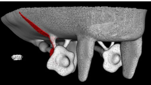
The increased capabilities of autonomous underwater vehicles (AUVs) have led to their use in inspecting underwater structures, such as docked ships (see Figure 1), submarines, and the ocean floor. Since these tasks are often time critical, and deployment time of AUVs is expensive, there is significant motivation to improve the efficiency of these autonomous inspection tasks. Coordinating the AUV in such scenarios is an active perception problem, where the path and sensor views must be planned to maximize information gained while minimizing time and/or energy (Bajcsy, 1988).
We will examine a subclass of active perception problems, which we refer to as active inspection, where an autonomous vehicle is inspecting the surface of a 3D structure represented by a closed mesh. In contrast with a large body of prior work, the focus of this paper is not on improving 3D reconstruction methods, but on properly modeling the uncertainty of a 3D reconstruction (resulting
∗
G. Hollinger and G. Sukhatme are with the Department of Computer Science, Viterbi School of Engineering, University of Southern California, Los Angeles, CA 90089 USA,{gahollin,gaurav}@usc.edu
†
B. Englot and F. Hover are with the Center for Ocean Engineering, Department of Mechanical Engineering, Massachusetts Institute of Technology, Cambridge, MA 02139 USA,{benglot,hover}@mit.edu
‡
U. Mitra is with the Department of Electrical Engineering, Viterbi School of Engineering, University of Southern California, Los Angeles, CA 90089 USA,[email protected]
Figure 1: Top: Visualization of an autonomous underwater vehicle inspecting a ship hull using profiling sonar. We propose constructing a 3D mesh from the sonar range data and modeling the mesh surface using non-parametric Bayesian regression, which provides a measure of uncertainty for planning informative inspection paths.
from sensor noise, data sparsity, and surface complexity) and planning informative paths for further data collection. Thus, the goal is to improve 3D reconstruction through better AUV path planning. In addition to choosing the most informative views, an autonomous vehicle may act adaptively by modifying its plan as new information becomes available. For instance, an AUV may receive fewer measurements than expected and would wish to modify its plan accordingly. However, adaptivity does not come without a cost: it requires significant onboard processing and also leads to robustness issues if unexpected events occur. A natural question to ask is whether we can bound the benefit of adaptivity for a given problem, which would guarantee the performance of the more robust non-adaptive strategies. Recent advances in stochastic optimization have enabled formal analysis of adaptivity through the derivation of adaptivity gaps (Goemans and Vondrak, 2006; Asadpour et al., 2009).
In the present paper, we apply adaptivity analysis to active inspection by formalizing the adaptivity gaps for information gain maximization and variance reduction. This analysis leads to a surprising result: minimizing cost subject to a constraint on information gain leads to an exponential adaptivity gap, while maximizing variance reduction subject to a constraint on cost leads to a constant factor adaptivity gap. The derivation of adaptivity gaps is novel for robotic inspection problems, and formalizing these gaps provides tools for principled design of both adaptive and non-adaptive algorithms.
An important component of active inspection is the development of a measure of uncertainty on the surface of the mesh. To this end, we discuss methods for generating closed surfaces that are robust to data sparsity and noise, and we propose modeling uncertainty using non-parametric Bayesian regression. Our method uses Gaussian Process Implicit Surfaces (Williams and Fitzgib-bon, 2007) with an augmented input vector (Thompson and Wettergreen, 2008). The input vector is augmented with the estimated surface normals found during mesh construction to yield higher uncertainty in areas of higher variability. We also apply local approximation methods (Vasudevan et al., 2009) to achieve scalability to large data sets. The resulting uncertainty measures provide principled objective functions for planning paths of an AUV for further inspection. We connect the related objective functions to problems in submodular optimization, which provides insight into the underlying structure of active perception problems.
mesh either from prior data or from an initial coarse inspection. Depending on the availability of such a mesh or the time cost in running the initial inspection, alternative methods that do not use a prior model may be more appropriate. In the present paper, we focus on cases where such a model is available, which allows the use of sophisticated methods for estimating the uncertainty of the reconstruction and the use of long-term planning for optimizing the future sensing actions of the vehicle.
The key novelties of this paper are (1) the derivation of both exponential and constant factor adaptivity gaps for different formulations of the active inspection problem, (2) the use of Gaussian Process Implicit Surfaces with augmented input vectors to provide a measure of uncertainty on mesh surfaces, and (3) the development of a probabilistic planner that maximizes uncertainty reduction while still providing coverage of the mesh surface. In addition to providing novel algorithms for improving inspection planning, we also provide insight into the potential benefit of adaptivity in such domains. This paper combines ideas that were originally introduced in two prior conference papers (Hollinger et al., 2011, 2012). The journal version contains additional simulations and new theoretical analysis showing the connection between active inspection and stochastic optimization. The remainder of this paper is organized as follows. We first discuss related work in active perception, 3D reconstruction, and informative path planning (Section 2). We then formulate the general active inspection problem (Section 3), discuss performance guarantees for scalable inspec-tion planning algorithms, and quantify adaptivity gaps for two formulainspec-tions of active inspecinspec-tion (Section 4). Next, we move to the example domain of ship hull inspection, and we present a complete solution in this domain. We propose methods for constructing closed 3D meshes from acoustic range data (Section 5.1), develop techniques to represent uncertainty on meshes by extend-ing Gaussian Process (GP) modelextend-ing (Section 5.2), and then formulate a probabilistic path planner for minimizing uncertainty based on probabilistic roadmaps (Section 5.3). To test our approach, we utilize ship hull inspection data from two data sets, and we show that the proposed path planning method successfully reduces uncertainty on the mesh surface (Section 6). Finally, we conclude and discuss avenues for future work (Section 7).
2
Related Work
The problem of active perception has been studied extensively in the computer vision community, dating back to early work in active vision (Bajcsy, 1988; Aloimonos et al., 1988) and next-best view planning (Connolly, 1985). While early work primarily optimized views using a geometric approach, later work incorporated probabilistic models into active perception systems (Arbel and Ferrie, 2001; Sipe and Casasent, 2002; Denzler and Brown, 2002).1 Such approaches have also been applied to depth maps in the context of medical imagery (Zhou et al., 2003). While different forms of uncertainty play a critical role in active vision, key distinctions in our work are the use of long-term planning and the analysis of adaptivity. In active inspection problems, selecting the next best observation, or even an initial ordering of informative observations, may not result in overall performance optimization. It is in this regard that we provide new analysis of the benefit of adaptivity and make connections to performance guarantees in submodular optimization and active learning. Our analysis is complementary to prior computer vision work and could potentially be
1
There are a number of additional active vision works relevant to the present paper. We direct the interested reader to Roy et al. (2004) and Chen et al. (2011) for surveys.
extended to many of these alternative frameworks.
In this paper, we connect two classical problems: active perception and sequential hypothesis testing. Sequential hypothesis testing arises when an observer must select a sequence of noisy experiments to determine the nature of an unknown (Wald, 1945). A key distinction between sequential hypothesis testing and active perception is that the type of experiment does not change in sequential testing, whereas in active perception we can select a number of possible “experiments” in the form of sensing actions. One of the first applications of sequential hypothesis testing to sensor placement applications was due to Cameron and Durrant-Whyte (1990). They discuss a Bayesian selection framework for identifying 2D images with multiple sensor placements. Their work provides a foundation for the formulation discussed in the current paper.
Many active perception problems can be seen as instances of informative path planning (Singh et al., 2009). Informative path planning optimizes the path of a robot to gain the maximal amount of information relative to some performance metric. It has been shown in several domains, including sensor placement (Krause and Guestrin, 2005) and target search (Hollinger et al., 2009), that many relevant metrics of informativeness satisfy the theoretical property of submodularity. Submodularity is a rigorous characterization of the intuitive notion of diminishing returns that arises in many information gathering applications. Analyzing problems using these tools provides formal hardness results, as well as performance bounds for efficient algorithms. Thus, we gain additional insight into the nature of active perception problems.
Recent advances in active learning have extended the property of submodularity to cases where the plan can be changed as new information is incorporated. The property of adaptive submodularity was introduced by Golovin and Krause (2011), which provides performance guarantees in many domains that allow for in situ decision making. Their recent work examines these theoretical properties in the context of a sequential hypothesis testing problem with noisy observations (Golovin et al., 2010). The idea of acting adaptively has also been examined in stochastic optimization and shown to provide increases in performance for stochastic covering (Goemans and Vondrak, 2006), knapsack (Dean et al., 2008), and signal detection (Naghshvar and Javidi, 2010). To our knowledge, these ideas have not been formally applied to robotics applications.
Acoustic range sensing, essential in the inspection of turbid-water environments, has been used to produce 3D point clouds throughout various underwater domains. Early work in 3D underwater mapping dates back more than a decade to the use of diver-held sonar devices that utilized an inertial measurement unit to help align subsequent images (am Ende, 2001). Such techniques inevitably suffer from drift over time, which can be mitigated through Simultaneous Localization and Mapping (SLAM) techniques (Fairfield et al., 2007). It is also possible to generate underwater maps without motion estimation through sophisticated techniques for accurate registration (Buelow and Birk, 2011; Pathak et al., 2010). Such approaches can also be combined with SLAM to produce even more accurate reconstructions (Pfingsthorn et al., 2012). Castellani et al. (2005) provided a complete system for underwater 3D reconstruction, which allows for online refinements during the mission. In their work, the vehicle is remotely controlled by a human operator, and the potential for autonomous operation is not explored.
For ground, air, and space applications, the predominant sensor for 3D reconstruction is laser-based ranging. Such sensors can yield high-resolution 3D point clouds (typically of sub-millimeter rather than sub-decimeter resolution), and specialized algorithms have been designed to generate watertight 3D mesh models from these high-resolution point clouds (Curless and Levoy, 1996; Hoppe et al., 1992). Recently, an increasing number of tools are being developed for processing
laser-based point clouds containing gaps, noise, and outliers (Huang et al., 2009; Weyrich et al., 2004). We apply a number of these techniques to improve the quality of 3D reconstruction in the underwater ship hull inspection domain.
These prior works demonstrate the feasibility of 3D reconstruction underwater as well as in terrestrial environments. However, they do not address the problems of determining the accuracy of the reconstruction, and they do not propose methods for coordinating autonomous vehicles to improve data collection. It is in this vein that we propose methods for representing 3D reconstruc-tion uncertainty using Gaussian Processes and we explore probabilistic moreconstruc-tion planning techniques for autonomous data acquisition.
To our knowledge, prior work has not considered the use of probabilistic regression for planning the inspection of a closed mesh. Similar problems, such as active 3D model acquisition (Chen and Li, 2005; Dunn et al., 2009), have been examined, primarily using geometric techniques. Krainin et al. (2011) proposed an information gain heuristic for acquiring a complete 3D model of an object, but they do not consider surface variability as part of their technique. Gaussian Processes have been used to define implicit surfaces for 2.5D surface estimation (Vasudevan et al., 2009) and grasping tasks (Williams and Fitzgibbon, 2007; Dragiev et al., 2011), but these techniques do not actively plan to reduce uncertainty on the surface.
A novelty of our approach is the use of surface normals as part of an augmented input vector to provide a better measure of surface uncertainty. The augmented input vector approach has been used to provide non-stationary kernels for Gaussian Processes (Pfingsten et al., 2006; Thompson and Wettergreen, 2008), though not in the context of surface modeling or with surface normal estimates. A similar idea of uncertainty-driven planning was proposed by Whaite and Ferrie (1997). They use a linear approximation of the surface, and they use the resulting covariance matrix as the measure of uncertainty. Gaussian Processes provide a more general uncertainty measure that is able to trade off between data sparsity and surface variability when estimating uncertainty.
3
Problem Formulation
Before presenting more specialized algorithms for underwater inspection domains, we will first propose a general formulation for the active inspection problem and analyze formal guarantees on adaptive and non-adaptive policies in these domains. Our formulation connects active inspection to the classical problem of sequential hypothesis testing (Wald, 1945). In sequential hypothesis testing, the goal is to determine the class of an unknown given a hypothesis space H = {h1, h2, . . .}. For
the case of mesh surface inspection, the hypothesis space is that of all possible mesh surfaces, an infinite and high-dimensional space. We let H be a random variable equal to the true surface.
We can observe the mesh surface from a set of possible configurations L = {L1, . . . Lm}, where
each configuration represents a location and orientation of the vehicle.2 There is a cost c(Li, Lj) of
moving from configuration Li to configuration Lj. In robotics applications, this cost is determined
by the kinematics of the vehicle and the dynamics of both the vehicle and environment. In addition, there is an observation cost c(Li) incurred when examining the surface at configuration Li (e.g.,
the time taken to perform a sonar scan).
There is also a set of target features F = {F1, . . . , Fk} that distinguishe between surface types.
2
We formulate the problem for the case of discrete vehicle configurations. If a continuous representation is available, a roadmap of possible configurations can be generated through sampling (see Section 5.3).
The target features represent points on the surface and their respective normal vectors. Each target feature Fiis a random variable, which may take on some values (e.g., discrete, or continuous). Using
characteristics of the sensor, viewing geometry, and/or training data, we can calculate a function G : L → F mapping viewing configurations to the features (i.e., points on the surface) which will be observed from those viewing configurations. In general, this mapping may be stochastic. The mapping from configuration to features is a key characteristic of robotics applications that differentiates our problem from the more common problem where the features can be observed directly (Golovin et al., 2010).
In standard hypothesis testing, we are given knowledge of a prior distribution for each class P (H), as well as a conditional probability for each feature given the class P (Fi| H). The conditional
distribution represents the probability of each feature taking on each of its possible values given the class. In general, these probabilities can be estimated via training data, but they may be difficult or even impossible to estimate directly for the case of surface inspection. The features that have been viewed evolve as the robot moves from configuration to configuration. At a given time t, the robot is at configuration L(t), and we observe realizations of some new features Ft ⊂ F . Let us define
F1:t := ∪ti=1Fias the features observed up until time t. We can now define the posterior distribution b(t) := P (H | F1:t). For the special case of conditionally independent features, the posterior
distribution can be calculated efficiently using standard recursive Bayesian inference (Thrun et al., 2005).
The goal is to find a policy π that takes a belief distribution b(t), current configuration L(t), and observation history F1:t and determines the next configuration from which to view the surface. The
dependence on the observation history and current distribution allows the policy to act adaptively as new information becomes available. When the observations are noisy, it will likely be impossible to determine the shape of an unknown surface with certainty. However, we can generate a policy that maximizes the expected information gain up to a time T given that we can calculate the features we would expect to observe:
JIG(π) = H(H) − H(H | π), (1)
where H(H) is the entropy of the prior and H(H | π) is the expected entropy after executing policy π.
An alternative formulation is to cast the problem as one of reducing the predicted variance of the surface estimate. After executing a policy π, we can estimate a variance function Vπ(x) for all
points x on the surface using a function approximation (e.g., a Gaussian Process). We can now define the following metric related to reducing the average variance reduction:
Jvar(π) =
Z
XV
0(x) − Vπ(x) dx. (2)
For a policy π, we set the measure of information quality J (π) to one of the above options, and we define a path cost c(π) = EH[c(π, h)] as the expected time to execute this policy (expected
traversal cost plus expected viewing cost). We will examine optimization problems of the following form:
π∗ = argmax π J (π) s.t. c(π) ≤ B, (3) π∗ = argmin π c(π) s.t. J (π) ≥ Q, (4)
where B and Q are budget and quality constraints respectively. We note that we can alternatively maximize the weighted sum αJ (π)−βc(π) with appropriate weighting constants using a Lagrangian relaxation (Fisher, 1981).
4
Theoretical Analysis
We next relate the surface inspection problem to recent advances in active learning theory that allow us to analyze the performance of both non-adaptive and adaptive policies. Prior work in active inspection does not provide tools for analyzing the performance of approximate solutions. With the goal of generating approximation guarantees for scalable algorithms, we provide a preliminary analysis of the theoretical properties of active inspection objective functions. In subsequent sections, we will apply these algorithms to the ship hull inspection domain and verify the theoretical analysis experimentally.
4.1 Performance Guarantees
A non-adaptive policy is one that generates an ordering of configurations to visit and does not change that ordering as features are observed. The non-adaptive policy will typically be easier to compute and implement, since it can potentially be computed offline and run without modification. Performance guarantees in non-adaptive domains often result from the objective function (i.e., the informativeness of the views) being monotone and submodular on the ground set of possible viewing configurations L. We will examine performance guarantees for maximization of reward functions J : 2L→ <+0 that satisfy the properties of monotonicity and submodularity.3
A set function is monotone if the objective never decreases by making more observations: Definition 1 A function J : 2L→ <+0 is called nondecreasing iff for all A, B ⊆ L, we have
A ⊆ B ⇒ J (A) ≤ J (B).
A set function is submodular if it satisfies the notion of diminishing returns. In our cases, the more views that have been examined, the less incremental benefit can be gained by selecting an additional view:
Definition 2 A function J : 2L→ <+0 is called submodular iff for all A, B ⊆ L and all singletons {e} ∈ L, we have
A ⊆ B ⇒ J (A ∪ e) − J (A) ≥ J (B ∪ e) − J (B). 3
The definition of J is overloaded here because J was previously defined on the space of policies. For the non-adaptive case, a policy is equivalent to a selection of viewing configurations. For the non-adaptive case, J can be seen as either a function of the adaptive policy or a function of the viewing configurations selected by the adaptive policy.
Information gain has been shown to be both monotone and submodular if the observations are conditionally independent given the class (Krause and Guestrin, 2005). Variance reduction has also been shown to be monotone and submodular in many cases (Das and Kempe, 2008). Let Agdy be the set of configurations visited by using a one-step look-ahead on the objective function. For non-adaptive policies subject to a cardinality constraint on observations without path constraints (e.g., when traversal costs between configurations are negligible compared to observation cost), we have the following performance guarantee when the objective is monotone and submodular: J (Agdy) ≥ (1 − 1/e)J (Aopt) (Krause and Guestrin, 2005).
When path constraints are considered, the recursive greedy algorithm, a modification of greedy planning that examines all possible middle configurations while constructing the path, can be utilized to generate a path Arg (Singh et al., 2009). The recursive greedy algorithm provides a per-formance guarantee of J (Arg) ≥ J (Aopt)/ log(|Aopt|), where |Aopt| is the number of configurations
visited on the optimal path. However, the recursive greedy algorithm requires pseudo-polynomial computation, which makes it infeasible for some application domains. To our knowledge, the devel-opment of a fully polynomial algorithm with performance guarantees in informative path planning domains with path constraints is still an open problem.
The performance guarantees described above do not directly apply to adaptive policies. An adaptive policy is one that determines the next configuration to select based on the observations at the previously visited configurations. Rather than a strict ordering of configurations, the re-sulting policy is a tree of configurations that branches on the observation history from the past configurations. The concept of adaptive submodularity (Golovin and Krause, 2011) allows for some performance guarantees to extend to adaptive policies as well. When the objective is adaptive sub-modular, as is the case for variance reduction with stochastic sensing (see Section 4.2.2), the one-step adaptive policy without path constraints is bounded as: J (Agdyadapt) ≥ (1 − 1/e)J (Aoptadapt). When information gain is considered, a reformulation of the problem is required to provide performance guarantees (i.e., information gain is not adaptive submodular). However, Golovin et al. (2010) show that the related Equivalence Class Determination Problem (ECDP) optimizes an adaptive submod-ular objective function and yields a logarithmic performance guarantee. The direct application of ECDP to active inspection is left for future work.
4.2 Benefit of Adaptivity
We now examine the benefit of adaptive selection of configurations in the active inspection domain. As described above, the non-adaptive policy will typically be easier to compute and implement, but the adaptive policy could potentially perform better. A natural question is whether we can quantify the amount of benefit to be gained from an adaptive policy for a given problem. If J (πadapt) is the objective value gained by an optimal adaptive policy and J (πnon−adapt) is the
objective value gained by an optimal non-adaptive policy, we wish to bound the adaptivity gap defined by J (πnon−adapt)/J (πadapt) for a minimization problem or J (πadapt)/J (πnon−adapt) for a
maximization problem (Goemans and Vondrak, 2006; Asadpour et al., 2009).
Throughout this section we will assume that observation cost c(Li) dominates traversal cost
c(Li, Lj). This assumption is valid if observation cost is high (e.g., the time to scan from a given
configuration is large) or if the views are sufficiently dense that total observation cost dominates. Analysis of adaptivity for domains where traversal cost dominates is a particularly interesting avenue for future work.
4.2.1 Large adaptivity gap for minimizing observation cost and constraining infor-mation gain
To begin our analysis of adaptivity, we consider the problem of minimizing the expected cost of observation subject to a hard constraint on information gain.
Problem 1 Given hypotheses H = {h1, h2, . . . , hn}, features F = {F1, F2, . . . , Fk}, configurations
L = {L1, . . . , Lm}, costs c(Li) for observing from configuration Li, and an objective J (π), we wish
to select a policy π such that:
π∗ = argmin
π
c(π) s.t. J (π) ≥ Q, (5) where J (π) := H(H) − H(H | π), c(π) := EH[c(π, h)], and Q is a scalar.
We now show that the optimal non-adaptive policy can require exponentially higher cost than an adaptive policy for an instance of this problem.
Theorem 1 Let πadapt be the optimal adaptive policy, and πnon−adapt be the optimal non-adaptive
policy. There is an instance of Problem 1 where c(πadapt) = log(n) and c(πnon−adapt) = n − 1, where
is n is the number of hypotheses.
Proof We adopt a proof by construction. Let the initial distribution of P (H) be uniform, and let Q = H(H) (i.e., the true hypothesis must be known with certainty). Let the features be observed directly through the corresponding configurations (i.e., G(Li) = Fi and m = k). Let there be n
hypotheses and m = n − 1 features. Assign a cost c(Li) = 1 for all configurations.
Let P (F1|hi) = 1 for all i ∈ {1, . . . , n/2} and P (F1|hi) = 0 for all i ∈ {n/2 + 1, . . . , n}. That is,
feature F1 is capable of deterministically differentiating between the first half and second half of
the hypotheses. P (F2|hi) = 1 for all i ∈ {1, . . . , n/4}, P (F2|hi) = 0 for all i ∈ {n/4 + 1, . . . , n/2},
and P (F2|hi) = 1/2 for all i ∈ {n/2 + 1, . . . , n}. That is, feature F2 is capable of deterministically
differentiating between the first fourth and second fourth of the hypothesis space, but gives no information about the rest of the hypotheses. Similarly, define P (F3|hi) = 1 for all i ∈ {n/2 +
1, . . . , 3n/4}, P (F3|hi) = 0 for all i ∈ {3n/4 + 1, . . . , n}, and P (F3|hi) = 1/2 for all i ∈ {1, . . . , n/2}.
The remaining features are defined that differentiate progressively smaller sets of hypotheses until each feature differentiates between two hypotheses.
The adaptive policy will select F1first. If F1 is realized positive, it will select F2. If F1is realized
negative, it will select F3. It will continue to do a binary search until log(n) features are selected.
The true hypothesis will now be known, resulting in zero entropy. In contrast, the non-adaptive policy must select all n − 1 features to ensure realizing the true hypothesis and reducing the entropy to zero.
The analysis in Theorem 1 shows that the adaptivity gap for this formulation is bounded below as Ω(n/ log(n)), which represents a significant potential benefit of acting adaptively, particularly as the number of hypotheses increases. For the case of an infinite (or arbitrarily large) number of hypotheses, as in surface inspection, the benefit for adaptivity for this formulation can be arbitrarily large. We also note that this adaptivity gap holds even when the mapping between configurations and features is deterministic. Next, we will examine the related problem of minimizing variance reduction with stochastic sensing.
4.2.2 Small adaptivity gap for maximizing variance reduction with stochastic sensing We now continue our adaptivity analysis to show a somewhat surprising result: the benefit of adaptivity is bounded by a constant factor when variance reduction is minimized subject to a constraint on observation cost. We utilize the more general result from Asadpour et al. (2009) to show that the adaptivity gap for variance reduction with uncertain sensing is equal to e/(e − 1) ≈ 1.58. This result holds for cases where maximizing the variance reduction is submodular and the mapping between sensing configurations and observed locations is independent for each sensing configuration. We now characterize the problem formally.
Problem 2 Given hypotheses H = {h1, h2, . . . , hn}, features F = {F1, F2, . . . , Fk}, configurations
L = {L1, . . . , Lm}, a stochastic mapping G : L → F , costs c(Li) for observing from configuration
Li, and an objective J (π), we wish to select a policy π such that:
π∗ = argmax
π
J (π) s.t. c(π) ≤ B, (6)
where J (π) :=RXV0(x) − Vπ(x) dx, c(π) := EH[c(π, h)], and B is a scalar.
We note that multiplicity in viewing configurations (i.e., sensing from a configuration multiple times) and target locations (i.e., viewing a target location multiple times) can be incorporated in this formulation by adding additional copies of each configuration or location to the appropriate vector. We assume the distribution of the stochastic mapping is known and is independent between sensors. The mapping may follow any arbitrary probability distribution. We will analyze the case where the object J is monotone submodular, which is often the case for variance reduction, particularly with a squared exponential kernel (see Das and Kempe (2008) for a rigorous characterization of these cases).
We now apply the result from prior work to derive an adaptivity gap for the problem above. Theorem 2 Let πadapt be the optimal adaptive policy, and πnon−adapt be the optimal non-adaptive
policy. The adaptivity gap J (πadapt)/J (πnon−adapt) for Problem 2 is equal to e/(e − 1) when J (π)
is monotone submodular.
Proof We show the result by casting the variance reduction problem as an instance of stochastic monotone submodular maximization (SMSM) (Asadpour et al., 2009).
The SMSM problem is defined by a set X = X1, . . . , Xnof n independent random variables over
a domain ∆. The distribution of realizations for each Xi is given by an independent function gi. Let
xidenote a realization of Xi, and let vector y = (ˆx1, . . . , ˆxn) denote a realization of set Y ⊂ X , where
ˆ
xi = xifor Xi∈ Y and ˆxi = 0 for Xi ∈ Y. For a function f : ∆/ n→ R+, we can define the stochastic
function F : 2X → R+ as F (Y) = E[f (y)], where y is a realization of Y and the expectation is
taken with respect to the joint distribution defined by the gi’s. Similarly, we can consider a subset
Z ⊂ X and a realization z of Z, which provides a conditional expectation E[f(y)|z], where yi = zi
if its corresponding random variable is in Y ∩ Z. Otherwise yi is chosen independently with respect
to the distribution defined by gi. We will denote this conditional expectation as F (Y, z). The set
function F is stochastic monotone submodular if F (·, z) is monotone submodular for every z. The SMSM problem is as follows: given the set X = X1, . . . , Xn of n independent random
2X → R+, find a subset S ∈ I that maximizes F , i.e., max
S∈IE[F (S)], where the expectation is taken over the probability distribution of the sets chosen by the policy.
For the case of variance reduction, we set F = Jvar as the variance reduction function, and
the domain ∆ as all possible subsets of features in F . For every instantiation z, this function is monotone submodular in the absence of suppressor variables (Das and Kempe, 2008). In such cases, F is stochastic monotone submodular because it is a convex combination of monotone sub-modular functions (i.e., an expectation). The viewing configurations L represent the set X , and each instantiation xi represents a vector vi ∈ 2F denoting the viewed features. The viewed set S is
fully defined by the collection of vectors vi. The function gi is determined by the known stochastic
mapping G. Finally, the matroid M = (L, A ⊆ L : |A| ≤ B) for budget B forms a uniform matroid. Thus, we have an instance of SMSM. Applying Theorem 1 from Asadpour et al. (2009) shows that the adaptivity gap is equal to e/(e − 1).
From the above result, we see that the adaptivity gap is equal to e/(e−1) ≈ 1.58 for the problem of variance reduction with stochastic sensing. Thus, the optimal adaptive policy will provide at most 1.58 times the variance reduction as the optimal non-adaptive policy. If we contrast this value with the Ω(n/log(n)) adaptivity gap from the previous section, we notice that recasting the problem as variance reduction reduces an exponential adaptivity gap to a constant factor. In the context of adaptive inspection, where both problems are similar in nature, this result is quite surprising. Based on theoretical analysis in this section, we would expect to see limited benefit from adaptivity for variance reduction problems. The experiments in the subsequent sections will confirm this trend.
5
Surface Reconstruction and Inspection Planning
Drawing on the theoretical analysis in the previous section, we will now discuss methods for per-forming informative inspections using ship hull inspection as an example domain. In this domain, an AUV is inspecting the submerged portion of a ship hull, and the goal is to plan the actions of the AUV to gather data that results in the best 3D reconstruction of the hull. We utilize the Bluefin-MIT Hovering Autonomous Underwater Vehicle (HAUV), which was designed for autonomous surveillance and inspection of in-water ships (Hover et al., 2007). The proposed algorithm follows the following steps, which are discussed in more detail in the subsequent sections:
1. Perform a coarse survey of the ship hull and determine an initial mesh reconstruction. For the purposes of this paper, we assume that this survey has already been performed. Methods for generating the initial mesh reconstruction through Poisson Reconstruction are described in Section 5.1.
2. Utilize Gaussian Process modeling to estimate the uncertainty on the surface of the initial mesh reconstruction as described in Section 5.2. These uncertainty estimates will help to guide further inspection and can be applied to any point cloud with surface normal estimates. 3. Plan subsequent viewing configurations for the HAUV to minimize the uncertainty in the
reconstruction. Section 5.3 discusses efficient methods for such planning using probabilistic roadmaps, rapidly exploring random trees, and TSP tours. The views are selected according to uncertainty reduction in the Gaussian Process. The planner also has the option to re-plan adaptively based on the new sensor readings.
The algorithm described above assumes that the HAUV has already completed a coarse survey of the ship hull, which provides an initial set of data points to use for constructing a 3D mesh and generating an uncertainty representation. If such a mesh is not available, or the cost of running the coarse survey is time prohibitive, online methods for improving the inspection that incorporate exploration should be used. The development of such methods is an interesting avenue for future work. Here we focus on the case where a preliminary mesh is available, and the goal is to utilize the mesh from the initial inspection to plan further inspection that improves the estimate of the surface’s shape.
In addition, we assume the vehicle is capable of high-quality localization, so the data gathered during the inspection accurately represents the geometry of the structure. Over short periods, relying on the HAUV’s DVL and IMU for localization is sufficient, but these sensors are subject to drift over time. Registration of camera images (Kim and Eustice, 2009) and 2D sonar images (Johannsson et al., 2010) has been used to provide accurate navigation over extended periods time; these measurements have also been integrated into a unified state estimation process for the HAUV (Hover et al., 2012). The incremental smoothing and mapping (iSAM) algorithm is used for state estimation (Kaess et al., 2008). So far, this capability has been used for hull-relative navigation, which is implemented over the flat and expansive forward areas of a ship. Efforts are currently in progress, however, to provide this capability for the seafloor-relative navigation used in inspecting the 3D structures at a ship’s stern.
In the present paper, we rely on dead reckoning that uses the DVL, IMU, and depth sensor for accurate navigation over short periods of time (the IMU drifts at a rate of ten degrees per hour). A Kalman filter is used to produce depth and attitude estimates using the IMU and depth sensor, and DVL velocities are integrated to provide x-y position estimates. More details on the localization system are provided in Hover et al. (2007).
5.1 Building 3D Models
We first address the problem of building 3D models from acoustic range data, which will later be used to derive a model of uncertainty for further inspection. Complex 3D structures are frequently encountered during hull inspections, particularly at the stern of the ship, where shafts, propellers, and rudders protrude from the hull. The HAUV uses a DIDSON sonar (Belcher et al., 2002) with a concentrator lens to sample acoustic range scans for 3D modeling of these complex ship structures. The vehicle is shown in Fig. 2 along with its navigation and sensing components.
To address the challenges of this 3D modeling task, we utilize several point cloud processing and surface construction tools from the field of laser-based modeling. All of the tools used to transform a fully dense point cloud into a 3D reconstruction can be accessed within Meshlab (Cignoni et al., 2008). A fully dense point cloud of a ship hull is first obtained by applying a simple outlier filter to the individual sonar frames collected over the course of an inspection mission. All pixels of intensity greater than a specified threshold are introduced into the point cloud, and referenced using the HAUV’s seafloor-relative navigation. Areas containing obvious noise and second returns are manually cropped out of the point cloud.
The fully dense point cloud is then sub-sampled (to about 10% of the original quantity of points) and partitioned into separate component point clouds. The partitions are selected based on the likelihood that they will yield individually well-formed surface reconstructions. Objects such as rudders, shafts, and propellers are thin objects that may not be captured in the final model without
Figure 2: Components of the Bluefin MIT-HAUV (left) and example deployment for inspection (right). The vehicle utilizes a DIDSON sonar to gather range scans of the ship hull. Localization is provided using a Doppler Velocity Log (DVL) assisted by an IMU. The thrusters provide fully-actuated navigation and station-keeping capabilities.
separate processing from the hull. Normal vectors are computed over the component point clouds, and some flat surfaces, for which only one of two sides was captured in the data, are duplicated. Both sub-sampling and estimation of normals are key steps in the processing sequence, found in practice to significantly impact the accuracy of the mesh (Huang et al., 2009). Sub-sampling generates a low-density, evenly-distributed set of points, and normals aid in defining the curvature of the surface.
The Poisson surface reconstruction algorithm (Kazhdan et al., 2006) is next applied to the oriented point clouds. Octree depth is selected to capture the detail of the ship structures without including excess roughness or curvature due to noise in the data. The component surfaces are merged back together, and a final Poisson surface reconstruction is computed over the components. If the mesh is used as a basis for high-resolution inspection planning, then it may be further subdivided to ensure the triangulation suits the granularity of the inspection task.
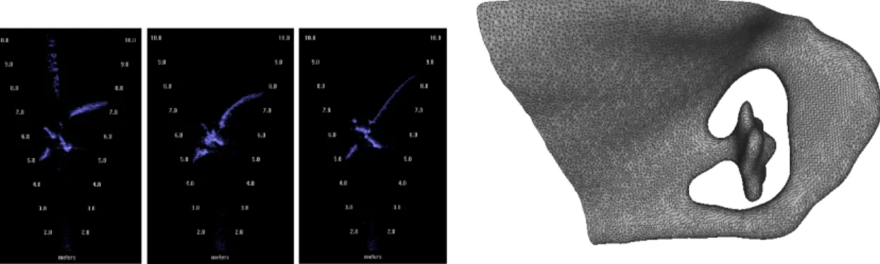
Fig. 3 depicts several representative range scans of a ship propeller, and the final 3D model of the ship’s stern produced from the same survey. Evident in the sonar frames is the noise which makes this modeling task difficult in comparison to laser-based modeling, requiring manual processing to remove noise and false returns from the data.
5.2 Representing Uncertainty
We now propose a method for representing uncertainty on the surface of a mesh reconstruction. The uncertainty will provide an estimate of the areas of the mesh surface that have been correctly reconstructed and those that are likely to be incorrect. We note that the proposed methods are not limited to the Poisson Reconstruction described in the previous section, and they can be applied to any mesh reconstruction method that provides a point cloud and surface normal vectors.
Given a mesh constructed from prior data, we propose modeling uncertainty on the surface of the mesh using non-parametric Bayesian regression. Specifically, we apply Gaussian process (GP) regression (Rasmussen and Williams, 2006), though any form of regression that generates a mean
Figure 3: An example of the raw data, and subsequent result, of the surface construction procedure. At left, three range scans featuring the hull, propeller, and rudder of the Nantucket Lightship, a historic ship 45 meters in length. These scans were collected in sequence as the HAUV dove with the running gear in view. At right, a 3D triangle mesh model from the complete survey of the Nantucket Lightship.
and variance could be used in our framework. A GP models a noisy process zi = f (xi) + ε, where
zi∈ R, xi ∈ Rd, and ε is Gaussian noise.
We are given some data of the form D = [(x1, z1), (x2, z2), . . . , (xn, zn)]. We will first formulate
the case of 2.5D surface reconstruction (i.e., the surface does not loop in on itself) and then relax this assumption in the following section. In the 2.5D case, xi is a point in the 2D plane (d = 2),
and zi represents the height of the surface at that point. We refer to the d × n matrix of xi vectors
as X and the vector of zi values as z.
The next step in defining a GP is to choose a covariance function to relate points in X. For surface reconstruction, the choice of the kernel is determined by the characteristics of the surface. We employ the commonly used squared exponential, which produces a smooth kernel that drops off with distance:
k(xi, xj) = σf2exp − d X k=1 wk(xik− xjk)2 ! . (7) The hyperparameter σ2
f represents the process noise, and each hyperparameter wk represent a
weighting for the dimension k. Once the kernel has been defined, combining the covariance values for all points into an n × n matrix K and adding a Gaussian observation noise hyperparameter σ2n yields cov(z) = K + σ2nI. We now wish to predict the mean function value (surface height) ¯f∗ and
variance V[f∗] at a selected point x∗ given the measured data:
¯
f∗ = kT∗(K + σ2nI)−1z, (8)
V[f∗] = k(x∗, x∗) − kT∗(K + σn2I)−1k∗, (9)
where k∗ is the covariance vector between the selected point x∗ and the training inputs X. This
model provides a mean and variance at all points on the surface in R2. In this model, the variance gives a measure of uncertainty based on the sparsity of the data and the hyperparameters.
5.2.1 Gaussian process implicit surfaces
The GP formulation described above is limited to 2.5D surfaces (i.e., a 2D input vector with the third dimension as the output vector). Thus, it is not possible to represent closed surfaces, such as a ship hull. To apply this type of uncertainty modeling to closed surfaces, we utilize Gaussian Process Implicit Surfaces (Williams and Fitzgibbon, 2007; Dragiev et al., 2011). The key idea is to represent the surface using a function that specifies whether a point in space is on the surface, outside the surface, or inside the surface. The implicit surface is defined as 0-level set of the real-valued function f where:
f : Rd→ R; f(x) = 0, x on surface > 0, x outside surface < 0, x inside surface (10)
In this framework, a measurement in the point cloud at a location x = (x, y, z) has a value of z = 0. We can add additional points outside the surface with z > 0 and points inside the surface with z < 0. The hyperparameter σf determines the tendency of the function to return to its mean
value, which is set to a number greater than zero (i.e., outside the surface). This framework allows the representation of any surface, regardless of its 3D complexity. In general, hyperparameters can be learned automatically from the data (Rasmussen and Williams, 2006). However, learning hyperparameters for implicit surfaces requires the generation points inside and outside the surface to provide a rich enough representation of the output space. We leave the generation of these points and improved hyperparameter estimation as an avenue for future work.
5.2.2 Augmented input vectors
A limitation of the above framework is that it uses a stationary kernel, which determines correlation between points solely based on their proximity in space. Thus, areas with dense data will have low uncertainty, and areas with sparse data will have high uncertainty. While data density is an important consideration when determining uncertainty, the amount of variability in an area should also be taken into account. For instance, the propeller of a ship hull has very complex geometry and will require a dense point cloud to reconstruct accurately.
To model surface variability, we utilize the augmented input vector approach to achieve a non-stationary kernel (Pfingsten et al., 2006; Thompson and Wettergreen, 2008). The idea is to modify the input vector by adding additional terms that affect the correlations between the data. One measure of variability is the change in surface normal between points. From the mesh constructed in Section 5.1, we have an estimate of the surface normals at each point on the surface. Using this information in the augmented input vector framework, we modify the input vector to be x0 = (x, y, z, ¯nx, ¯ny, ¯nz), where ¯nx, ¯ny, and ¯nz are the x, y, and z components of the surface normal
of the mesh at that point. We scale the surface normal to its unit vector, which reduces the possible values in the augmented input space to those between zero and one.
The weighting hyperparameters, denoted above as wk, can be adjusted to modify the effect of
spatial correlation and surface normal correlation. By modifying these hyperparameters, the user can specify how much uncertainty is applied for variable surface normals versus sparse data. If the spatial correlations are weighted more, areas with sparse data will become more uncertain. Conversely, if the surface normal correlations are weighted more, areas with high surface normal variability will become more uncertain.
5.2.3 Local approximation
The final issue to address is scalability. The full Gaussian Process models requires O(n3) computa-tion to calculate the funccomputa-tion mean and variance, which becomes intractable for point clouds larger than a few thousand points. To address this problem, we utilize a local approximation method us-ing KD-trees (Vasudevan et al., 2009). The idea is to store all points in a KD-tree and then apply the GP locally to a fixed number of points near the test point. This method allows for scalability to large data sets.
The drawbacks of this approach are that a separate kernel matrix must be computed for each input point, and the entire point cloud is not used for mean and variance estimation. However, depending on the length scale, far away points often have very low correlation and do not contribute significantly to the final output. We note that in prior work, this approach was not utilized in conjunction with implicit surfaces or augmented input vectors.
5.3 Inspection Planning
We now describe methods for planning the path of an AUV to minimize uncertainty in the mesh reconstruction. To plan the path of the vehicle, we utilize the sampling-based redundant roadmap method proposed in our prior work (Englot and Hover, 2011). We sample a number of configura-tions from which the vehicle can view the surface of the mesh, and we ensure that these viewing configurations are redundant (i.e., each point on the mesh is viewed some minimum number of times). After sampling is complete, viewing configurations from the roadmap are iteratively se-lected as waypoints for the inspection; they are chosen using one of three approaches described in the following section. The motivation for the greedy selection of viewing configurations stems from the performance guarantees described in Section 4.1. Waypoints are added until a specified number of views has been reached or a threshold on expected uncertainty reduction is acquired.
Once the set of waypoints has been selected, the Traveling Salesperson Problem (TSP) is approx-imated to find a low-cost tour which visits all of the designated viewing configurations. Initially, we assume that all point-to-point paths are represented by the Euclidean distances between the (x, y, z) coordinates of the configuration. The Christofides heuristic (Christofides, 1976) is implemented to obtain an initial solution which, for the metric TSP, falls within three halves of the optimal solution cost. The chained Lin-Kernighan heuristic (Applegate et al., 2006) is then applied to this solution for a designated period of time to reduce the length of the tour. All edges selected for the tour are collision-checked using the Rapidly-Exploring Random Tree (RRT) algorithm, Euclidean distances are replaced with the costs of feasible point-to-point paths, and the TSP is iteratively recomputed until the solution stabilizes (see (Englot and Hover, 2011) for more detail).
We assume that the vehicle does not collect data while moving between viewing configurations; this is intended to accommodate the servoing precision of the HAUV. The vehicle can stabilize at a waypoint with high precision, but the precise execution of point-to-point paths in the presence of ocean disturbances is harder to guarantee. We also note that the HAUV is stable when it hovers, and the speed of the vehicle is constant along the path, which further motivates this abstraction.
6
Simulations and Experiments
We test our proposed methods using ship hull inspection data from the Bluefin-MIT HAUV (see Section 5.1). This section examines two data sets: the Nantucket Lightship and the SS Curtiss, which first appeared in our prior conference paper (Englot and Hover, 2011). The Nantucket data set is composed of 21,246 points and was used to create a 42,088 triangle mesh with a bounding box of 6.3 m × 6.9 m × 4.4 m. The larger Curtiss data set contains 107,712 points and was used to create a 214,419 triangle mesh with a bounding box of 7.9 m × 15.3 m × 8.7 m.
We first examine the effect of the augmented input vectors on the uncertainty estimates. The GP hyperparameters were set to σf = 1.0 and σn= 0.1, based on the sensor noise model and the
mesh shape prior. The weighting hyperparameters were set to wk = 1 for all k, which provides
equal weighting of data sparsity and surface variability components in the kernel. Through the use of the KD-tree local approximation with 100 adjacent points, computation was completed in approximately 1 minute for the Nantucket data set and 3 minutes for the Curtiss data set on a 3.2 GHz Intel i7 processor with 9 GB of RAM.
Fig. 4 shows a comparison of uncertainty on the surface of the two meshes with and without augmented input vectors. Utilizing the surface normals as part of an augmented input vector incor-porates surface variability into the uncertainty prediction. As a result, areas with high variability require denser data to provide low uncertainty. For instance, parts of the propeller were incorrectly fused in the mesh reconstruction. The augmented input vector method shows high uncertainty at those locations on the mesh, demonstrating the need for further inspection. Since ground truth is not available, it is not possible to provide a quantitative comparison of the two uncertainty metrics using the ship hull data. However, the augmented input vector approach shows a stronger correlation to true error when run on simple benchmark meshes (not shown here).
We now quantify the benefit of utilizing uncertainty when planning inspection paths for the HAUV. For comparison, we assume the following sensor model, which is based on the inspection strategy for high-resolution surveying with the DIDSON. At each viewing configuration, which is defined by the position (x, y, z) and the heading angle θ, the HAUV is assumed to sweep the DIDSON sonar through a full 180 degrees in pitch. An individual DIDSON frame spans thirty degrees in vehicle-relative heading and has a tunable minimum and maximum range. The total range of a DIDSON scan determines the resolution of the scan, and high-resolution surveying is possible when short ranges are sampled. Here we assume the DIDSON scan spans a range of 1−4 m from the robot.
Inspection tours are found by first generating a redundant roadmap of possible views (see Section 5.3). Viewing configurations are then selected greedily from the roadmap using one of three methods: (1) coverage-biased: views are selected that maximize the number of new points observed, (2) uncertainty-biased: views are chosen to maximize the expected variance reduction on the surface, and (3) random selection: each point is selected uniformly. In all cases, viewing configurations that have already been selected are excluded from consideration. The coverage-biased method represents the state of the art in inspection planning as described in our prior work (Englot and Hover, 2011). The random view selection method provides a baseline inspection strategy that does not account for uncertainty reduction (e.g., those executed in much of the prior work in 3D reconstruction). For the uncertainty reduction method, it is computationally difficult to calculate the exact variance reduction for all possible viewing configurations. Instead, we approximate the variance reduction at each point on the surface as Vn(x) = V0(x) exp(−n/α), where V0(x) is the
(a) SS Curtis without augmented input vectors (b) SS Curtis with augmented input vectors
(c) Nantucket without augmented input vectors (d) Nantucket with augmented input vectors
Figure 4: Comparison of normalized uncertainty on the surface of the SS Curtiss (top) and Nan-tucket Lightship (bottom) meshes using a squared exponential kernel without augmented input vectors (left) and with augmented input vectors (right). Red areas are high uncertainty, and blue areas are low uncertainty. When the augmented input vectors are used, the uncertainty measure takes into account both data sparsity and surface complexity to provide a better prediction of the error in the reconstruction. This figure is best viewed in color.
initial uncertainty at point x, n is the number of times the point has been viewed in the plan, and α is a length scale parameter. The length scale parameter was set to α = 1.0 based on fitting to test runs where the exact reduction was calculated. For all three methods, the same redundant roadmap was used to provide candidate views.
After views are selected, the sampled points are then connected using the TSP/RRT method described in Section 5.3. This method generates a complete inspection path that can be executed by the vehicle. The total mission time is calculated assuming that the AUV requires 5 seconds to perform a scan from a viewing configuration and moves at a speed of 0.25 m/s. These numbers are taken directly from the experimental trials with the Bluefin-MIT HAUV. To evaluate the quality of the inspection paths, simulated measurements are generated by creating additional data points on the viewed parts of the mesh, and the surface normals of the new points are estimated from the original mesh. An estimate of expected uncertainty is then calculated by re-running the GP and determining the reduction in variance on the original points. The expected uncertainty reduction is a unitless quantity, which incorporates both data sparsity and surface variability.
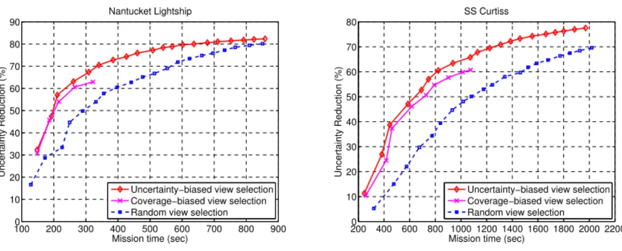
Fig. 5 shows a quantitative comparison of the three view selection methods. We see that view selection based on uncertainty reduction leads to greater reduction in variance for a given mission time. The coverage-biased selection method provides competitive uncertainty reduction for shorter paths (i.e., good coverage implicitly leads to good uncertainty reduction), but it does not allow for
1000 200 300 400 500 600 700 800 900 10 20 30 40 50 60 70 80 90
Mission time (sec)
Uncertainty Reduction (%)
Nantucket Lightship
Uncertainty−biased view selection Coverage−biased view selection Random view selection
2000 400 600 800 1000 1200 1400 1600 1800 2000 2200 10 20 30 40 50 60 70 80
Mission time (sec)
Uncertainty Reduction (%)
SS Curtiss
Uncertainty−biased view selection Coverage−biased view selection Random view selection
Figure 5: Mission time versus expected uncertainty reduction for inspection simulations. Uncertainty-biased view selection provides improved uncertainty reduction for a given mission time. Coverage-biased view selection does not allow for planning after full coverage is achieved, while the other methods continue to reduce uncertainty. Uncertainty reduction is a unitless quantity that takes into account data sparsity and surface variability; it is displayed as a percent reduction from its initial value.
(a) Nantucket Lightship (b) SS Curtiss
Figure 6: Planned inspection paths on two ship hull mesh data sets. Uncertainty-biased view selection provides an inspection path that views areas with sparse data and high variability. This figure is best viewed in color.
continued planning after full coverage is achieved. The performance of the random selection method improves (versus the uncertainty-biased method) as mission time increases, due to the amount of possible uncertainty reduction being finite. In the larger mesh, random view selection does not perform as well, even with long mission times. Fig. 6 shows example paths on each data set using the uncertainty-biased method.
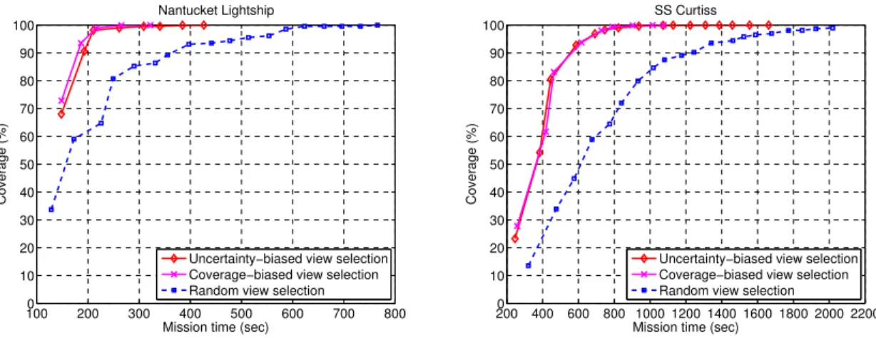
It is expected that the method that takes into account uncertainty would lead to greater variance reduction. However, we may be sacrificing some surface coverage to achieve this additional uncer-tainty reduction. Fig. 7 shows a comparison of the mission time vs. percent coverage for the three view selection methods. We see that the uncertainty reduction method converges quickly to greater
1000 200 300 400 500 600 700 800 10 20 30 40 50 60 70 80 90 100
Mission time (sec)
Coverage (%)
Nantucket Lightship
Uncertainty−biased view selection Coverage−biased view selection Random view selection
2000 400 600 800 1000 1200 1400 1600 1800 2000 2200 10 20 30 40 50 60 70 80 90 100
Mission time (sec)
Coverage (%)
SS Curtiss
Uncertainty−biased view selection Coverage−biased view selection Random view selection
Figure 7: Mission time versus percent coverage for inspection simulations. Plots are truncated after full coverage is achieved. Coverage-biased view selection and uncertainty-biased view selection both achieve full coverage. Random view selection does not achieve full coverage on the SS Curtiss mesh.
than 99% coverage, and reaches 100% coverage long before random sampling.4 Uncertainty-biased view selection gets to 99% coverage nearly as quickly as coverage-biased view selection, requiring only 41 seconds longer on the Nantucket mesh and 31 seconds longer on the Curtiss mesh, and it does so with a greater reduction in uncertainty. Thus, the uncertainty reduction method provides both high levels of coverage and improved uncertainty reduction for a given mission time.
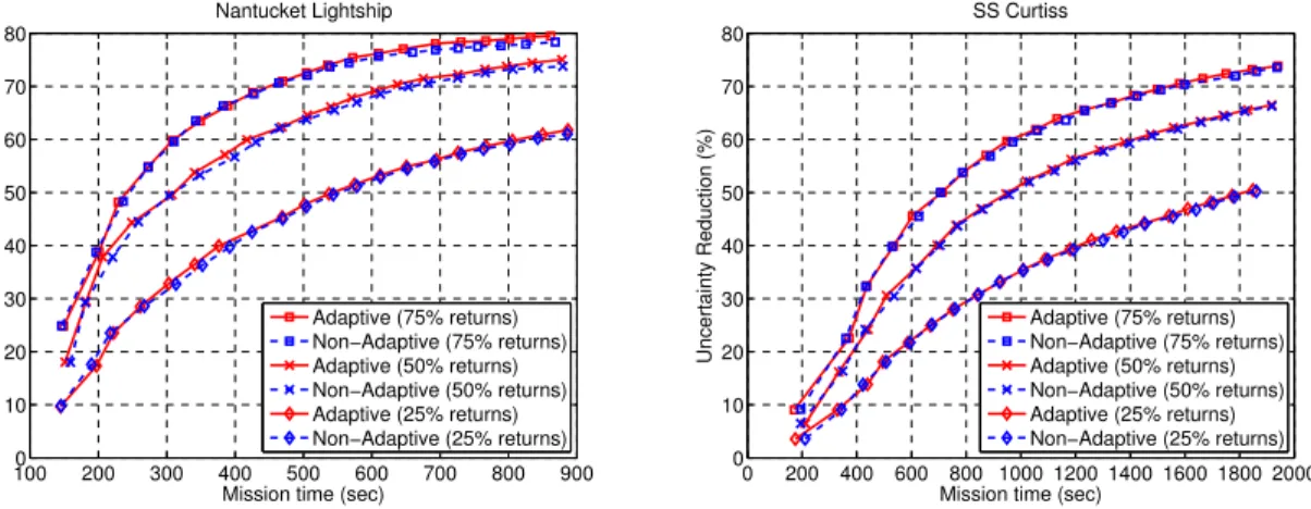
Finally, we examine the case where the sensor readings received by the AUV are no longer deterministic. We model stochasticity in the sensor readings by giving each viewed point on the surface a fixed probability of failing to return a measurement (i.e., a data point is not created in the new point cloud). As the failure probability is increased, we would expect the uncertainty reduction to suffer, due to the difficulty in acquiring data about the surface. For scenarios with stochastic sensor noise, we have the option to act adaptively, by choosing the next view based on the actual sensor readings received from the previous view. Alternatively, we can utilize a non-adaptive policy that computes the entire path based on the expected measurements received at each viewed points (assuming the model for sensor stochasticity is known). Fig. 8 compares these two methods for varying levels of sensor stochasticity.
Without considering the theoretical results in Section 4, the simulation results in Fig. 8 are surprising. The adaptive policy performs only marginally better than the non-adaptive policy, even for the case of high sensor stochasticity. However, if we consider the simulation results in the context of Theorem 2, we see that variance reduction in GPs with stochastic sensing has a relatively small adaptivity gap. Thus, we would predict the benefit of adaptivity to be small. The simulations confirm this prediction. Based on these results, we can utilize the non-adaptive strategy and still achieve competitive uncertainty reduction without the additional computation on the vehicle and robustness concerns of the adaptive strategy.
4
We note that since variance reduction is monotonic, uncertainty-biased view selection is guaranteed to achieve 100% coverage in the limit.
1000 200 300 400 500 600 700 800 900 10 20 30 40 50 60 70 80
Mission time (sec)
Uncertainty Reduction (%) Nantucket Lightship Adaptive (75% returns) Non−Adaptive (75% returns) Adaptive (50% returns) Non−Adaptive (50% returns) Adaptive (25% returns) Non−Adaptive (25% returns) 0 200 400 600 800 1000 1200 1400 1600 1800 2000 0 10 20 30 40 50 60 70 80
Mission time (sec)
Uncertainty Reduction (%) SS Curtiss Adaptive (75% returns) Non−Adaptive (75% returns) Adaptive (50% returns) Non−Adaptive (50% returns) Adaptive (25% returns) Non−Adaptive (25% returns)
Figure 8: Mission time versus expected uncertainty reduction for inspection simulations with dif-ferent levels of stochasticity in the sensor model. The non-adaptive strategy provides competitive performance with the adaptive strategy, as predicted by the small adaptivity gap.
7
Conclusions and Future Work
We have presented algorithms for efficiently inspecting an underwater structure using an AUV. Our theoretical analysis has shown that the potential benefit of adaptivity can be reduced from exponential to a constant factor by changing the problem from cost minimization with a constraint on information gain to variance reduction with a constraint on cost. This analysis allows the use of more robust, non-adaptive algorithms that perform competitively with adaptive algorithms, and it moves us towards formal analysis of active perception through connections to stochastic optimiza-tion and submodularity. The applicaoptimiza-tion of formal adaptivity analysis to active inspecoptimiza-tion is a new idea, and it is potentially applicable to other domains within the active perception framework.
We have also shown that it is possible to construct closed 3D meshes from noisy, low-resolution acoustic ranging data, and we have proposed methods for modeling uncertainty on the surface of the mesh using an extension to Gaussian Processes. Our techniques utilize surface normals from the 3D mesh to develop estimates of uncertainty that account for both data sparsity and high surface variability, and we achieve scalability to large environments through the use of local approximation methods. Our proposed probabilistic path planning algorithm generates views that effectively reduce the uncertainty on the surface in an efficient manner. Such analysis allows us to gain better understanding of the problem domain and to design principled algorithms for coordinating the sensing actions of autonomous underwater vehicles.
The small adaptivity gap derived here for the variance reduction case relies on the assumptions of submodularity, monotonicity, and the availability of a stochastic viewing function. In addition, it applies to cases where the mission cost is dominated by observation cost (i.e., the vehicle spends more time taking scans than moving between locations). In the domain discussed here, these assumptions hold; however, in other domains they may be violated. In such cases, it becomes increasingly important to determine cases where adaptivity is beneficial and to adjust accordingly. Such analysis motivates the development of algorithms that selectively adapt to maximize inspection efficiency.
corre-lations between points on the mesh surface. The neural network kernel has been employed in prior work and was shown to provide improved performance for modeling discontinuous surfaces (Va-sudevan et al., 2009). However, this kernel does not have a simple geometric interpretation, and its direct application to the implicit surface model does not produce reasonable uncertainty predic-tions. The automatic determination of hyperparameters for Gaussian Process Implicit Surfaces is another area for future work. To learn these automatically, a method would need to be developed to generate points both inside and outside the surface. The weighting hyperparameters in the augmented kernel that trade between data sparsity and surface variability also require additional information to constrain. For instance, a measure of data sparsity vs. surface variability and their respective effect on potential mesh error would allow for principled learning of these weightings.
Additional open problems include further theoretical analysis of performance guarantees, par-ticularly in the case of path constraints. The algorithm utilized in this paper selects views based on uncertainty reduction and then connects them using a TSP/RRT planner. A planner that utilizes the path costs when planning the view selection could potentially perform better, particularly in the case of a small number of views. Another future avenue is the development of a planner that provides a tradeoff between uncertainty reduction and surface coverage, both of which are useful metrics for inspection success. Such techniques would be particularly useful at higher levels of data sparsity and noise, where the active inspection methods have the potential to provide even greater improvement. Finally, the analysis in this paper has applications beyond underwater inspection. Tasks such as ecological monitoring, reconnaissance, and surveillance are just a few domains that would benefit from active planning for the most informed views and formal analysis of adaptivity. Through better control of the information we receive, we can improve the understanding of the world that we gain from robotic perception.
Acknowledgments
The authors gratefully acknowledge Jonathan Binney, Jnaneshwar Das, Arvind Pereira, and Hordur Heidarsson at the University of Southern California for their insightful comments. This work utilized a number of open source libraries, including the Armadillo Linear Algebra Library, the Open Motion Planning Library (OMPL), the Open Scene Graph Library, and the Approximate Nearest Neighbor (ANN) Library, and the Concorde TSP Library.
Funding
This research has been funded in part by the following grants: Office of Naval Research (ONR) N00014-09-1-0700, ONR N00014-07-1-00738, ONR N00014-06-10043, National Science Foundation (NSF) 0831728, NSF CCR-0120778, and NSF CNS-1035866.
References
Aloimonos, Y., Weiss, I., and Bandopadhyay, A. (1988). Active vision. International Journal of Computer Vision, 1(4):333–356.
am Ende, B. A. (2001). 3D mapping of underwater caves. IEEE Computer Graphics and Applications, 21(2):14–20.
Applegate, D. L., Bixby, R. E., Chv´atal, V., and Cook, W. J. (2006). The Traveling Salesman Problem: A Computational Study. Princeton Univ. Press.
Arbel, T. and Ferrie, F. P. (2001). Entropy-based gaze planning. Image and Vision Computing, 19(11):779– 786.
Asadpour, A., Nazerzadeh, H., and Saberi, A. (2009). Maximizing stochastic monotone submodular func-tions. Technical Report 0908.2788v1 [math.OC], arXiv Repository.
Bajcsy, R. (1988). Active perception. Proc. IEEE, Special Issue on Computer Vision, 76(8):966–1005.
Belcher, E., Hanot, W., and Burch, J. (2002). Dual-frequency identification sonar (DIDSON). In Proc. Int. Symp. Underwater Technology, pages 187–192.
Buelow, H. and Birk, A. (2011). Spectral registration of noisy sonar data for underwater 3D mapping. Autonomous Robots, 30(3):307–331.
Cameron, A. and Durrant-Whyte, H. (1990). A Bayesian approach to optimal sensor placement. Int. J. Robotics Research, 9(5):70–88.
Castellani, U., Fusiello, A., Murino, V., Papaleo, L., Puppo, E., and Pittore, M. (2005). A complete system for on-line modelling of acoustic images. Image Communication Journal, 20(9–10):832–852.
Chen, S., Li, Y., and Kwok, N. M. (2011). Active vision in robotic systems: A survey of recent developments. Int. J. Robotics Research, 30(11):1343–1377.
Chen, S. Y. and Li, Y. F. (2005). Vision sensor planning for 3-D model acquisition. IEEE Trans. Systems, Man, and Cybernetics, 35(5):894–904.
Christofides, N. (1976). Worst-case analysis of a new heuristic for the traveling salesman problem. Technical Report CS-93-13, Computer Science Dept., Carnegie Mellon Univ.
Cignoni, P., Corsini, M., and Ranzuglia, G. (2008). Meshlab: An open-source 3D mesh processing system. ERCIM News, 73:45–46.
Connolly, C. (1985). The determination of next best views. In Proc. IEEE Conf. Robotics and Automation, pages 432–435.
Curless, B. and Levoy, M. (1996). A volumetric method for building complex models from range images. In Proc. Conf. Computer Graphics and Interactive Techniques, pages 303–312.
Das, A. and Kempe, D. (2008). Algorithms for subset selection in linear regression. In Proc. ACM Symp. Theory of Computing, pages 45–54.
Dean, B., Goemans, M., and Vondrak, J. (2008). Approximating the stochastic knapsack: the benefit of adaptivity. Mathematics of Operations Research, 33(4):945–964.
Denzler, J. and Brown, C. (2002). Information theoretic sensor data selection for active object recognition and state estimation. IEEE Trans. Pattern Analysis and Machine Intelligence, 24(2):145–157.
Dragiev, S., Toussaint, M., and Gienger, M. (2011). Gaussian process implicit surfaces for shape estimation and grasping. In IEEE Int. Conf. Robotics and Automation, pages 9–13.
Dunn, E., van den Berg, J., and Frahm, J.-M. (2009). Developing visual sensing strategies through next best view planning. In Proc. IEEE/RSJ Int. Conf. Intelligent Robots and Systems, pages 4001–4008.