CoolEmAll D2.4 First release of the simulation and visualisation toolkit

(1)

HAL Id: hal-01818196

https://hal.archives-ouvertes.fr/hal-01818196

Submitted on 18 Jun 2018

HAL is a multi-disciplinary open access

archive for the deposit and dissemination of sci-entific research documents, whether they are pub-lished or not. The documents may come from teaching and research institutions in France or abroad, or from public or private research centers.

L’archive ouverte pluridisciplinaire HAL, est destinée au dépôt et à la diffusion de documents scientifiques de niveau recherche, publiés ou non, émanant des établissements d’enseignement et de recherche français ou étrangers, des laboratoires publics ou privés.

CoolEmAll D2.4 First release of the simulation and

visualisation toolkit

Daniel Rathgeb, Eugen Volk, Yosandra Sandoval, Georges da Costa, Thomas

Zilio, Micha Vor Dem Berge, Wojciech Piatek

To cite this version:

Daniel Rathgeb, Eugen Volk, Yosandra Sandoval, Georges da Costa, Thomas Zilio, et al.. CoolEmAll D2.4 First release of the simulation and visualisation toolkit. [Research Report] IRIT-Institut de recherche en informatique de Toulouse. 2013. �hal-01818196�

(2)

Project acronym: CoolEmAll

Project full title: Platform for optimising the design and

operation of modular configurable IT infrastructures and

facilities with resource-efficient cooling

D2.4 First release of the simulation and

visualisation toolkit

Authors: Daniel Rathgeb, Eugen Volk (HLRS)

Version: 1.0

(3)

Deliverable Number: D2.4 Contractual Date of Delivery: 31/03/2013 Actual Date of Delivery: 30/03/2013

Title of Deliverable: First release of the simulation and visualisation toolkit Dissemination Level: Public

WP contributing to the

Deliverable: WP 2

Authors: Daniel Rathgeb, Eugen Volk (HLRS) Co-Authors: Yosandra Sandoval (HLRS)

Georges da Costa (IRIT) Thomas Zilio (IRIT)

Micha vor dem Berge (Christmann) Wojciech Piatek (PSNC)

History

Version Date Author Comments

0.1 17.02.13 Eugen Volk (HLRS) Template

0.2 01.03.13 Daniel Rathgeb (HLRS) Skeleton

0.3 04.03.13 Eugen Volk (HLRS) Update Skeleton

0.4 07.03.13 Georges da Costa (IRIT) Application Profiler 0.5 08.03.13 Micha vor dem Berge

(Christmann)

DEBB Configurator 0.6 08.03.13 Wojciech Piatek (PSNC) DCworms

0.7 11.03.13 Thomas Zilio (IRIT) Metric Calculator 0.8 12.03.13 Yosandra Sandoval (HLRS) CoolEmAll Database 0.9 13.3.13 Daniel Rathgeb, Eugen Volk

(HLRS) Merging of contributions

091 14.03.13 Eugen Volk update

0.92 15.03.13 Review by Andrew Donogue (451G)

(4)

0.93 19.03.13 Laura Sisó (IREC) review

0.94 20.03.13 Daniel Rathgeb (HLRS) Adressing review comments

0.95 25.03.13 Eugen Volk (HLRS) Adressing review comments

0.96 26.3.2013 Daniel Rathgeb (HLRS) Adding partner contributions

(5)

Approval

Date Name Signature 15.03.13 Andrew Donogue Donogue

20.03.13 Laura Sisó Sisó

29.03.13 Eugen Volk Volk

Abstract

This deliverable describes the realisation of the first prototype of the simulation, visualisation and decision support toolkit and the interaction of its components. It further describes the usage and the tests of the components of the 1st_{Prototype of}

the SVD toolkit. Another focus of this deliverable is describing the heterogeneous deployment architecture of the SVD toolkit and the invoking of the different components for performing an automatic simulation.

This deliverable is split into four major parts. Each part describes the different properties of the individual components. Special focus is put on the distributed deployment architecture, realization, usage and tests of this 1st_prototype.

Keywords

First SVD toolkit prototype,OpenFOAM, CFD, Workload simulator, DCworms, Database, deployment, Repository, Simulation

(6)

List of Figures

Figure 2-1: SVD Toolkit - Architecture overview ... 11

Figure 2-2 Database Table Structure ... 17

Figure 4-1: Power usage chart generated for the DCWoRMS simulation ... 42

Figure 4-2: velocity and temperature distribution inside RECS ... 43

Figure 4-3: velocity and temperature distribution inside a compute room ... 44

List of Tables

Table 2-1: Components overview ... 11

Table 2-2: Software dependency list for SVN ... 13

Table 2-3: experiment-configuration ... 15

Table 2-4: Trial configuration ... 16

Table 2-5: Software dependency list for Python Wrapper ... 18

Table 2-6: Software dependency list for DCWoRMS ... 20

Table 2-7: Software dependency list for CFD ... 22

Table 2-8: Software dependency list for CFD ... 25

Table 2-9: Software dependency list for Metric Calculator ... 26

Table 3-1: Workload and resource management plugins/policies available within DCworms ... 31

Table 3-2: Energy and thermal plugins available within DCworms ... 32

Table 3-3: Application performance plugins available within DCWoRMS ... 33

(9)

List of abbreviations

API Application Programming Interface CFD Computational Fluid Dynamics

COVISE Collaborative Visualisation and Simulation Environment DCWoRMS Data Center Workload and Resource Management Simulator DEBB Data Centre Efficiency Building Block

GPL General Public License

LGPL GNU Lesser General Public License GSSIM Grid Scheduling Simulator

GUI Graphical User Interface GWF Grid Workload Format IP Internet Protocol

MOP Module Operation Platform

PLMXML eXtensible Markup Language for Product Lifecycle Management SVD Simulation Visualisation and Decision support toolkit

SVN Apache Subversion software versioning and revision control system SWF Standard Workload Format

STL Surface Tesselation Language

TIMaCS Tools for Intelligent System Management of Very Large Computing Systems

URL Uniform Resource Locator

(10)

1 Introduction

This deliverable describes the realization of the first prototype of the Simulation, Visualization and Decision Support Toolkit (SVD Toolkit). The SVD Toolkit is tool to help design more energy efficient data centres and optimize existing data centres to operate more energy efficient. This is done in several different consecutive steps. First, different application profiles are calculated. These application profiles resemble the requirements normal applications usually have. With these application profiles synthetic workloads are generated and used to determine a power usage of the individual hardware components. These results are used as input for CFD (Computational Fluid Dynamics) calculation. All results are stored in a central database. Additional results are obtained by conducting several characteristic trials, so that all results can be verified.

Another aim of this deliverable is to point out the realization of the interconnection points between different contributors and components. Special focus of this deliverable is also put into describing the usage of the prototype for conducting tests. The first prototype is supposed to deliver full productivity capabilities with minor shortcuts in user interface requests and speed of execution.

The SVD toolkit components described in this deliverable can be downloaded from the project-website [SVD Toolkit].

2 Realisation

The 1st prototype consists of several different components. The development for each component is done individually, although interaction between all components and a seamless workflow is ensured. This approach grants the user in this early step the possibility to use each of its components on its own. But because of focusing on the interfaces between the individual components of the first prototype these components work together seamlessly even in this early stage. The realization of the CFD-part of the SVD-toolkit first prototype is done as a command line interface. With the execution of a single command the user can do all the simulation automatically. The software relies, even in this early stage, fully on the Open Source Package OpenFOAM as a CFD solver.

2.1 Deployment architecture

For this first prototype, the database is the central interaction point where all of the considered components meet. This is for now the point for storing and retrieving data and communications between invoked components.

The deployment of SVD toolkit components and interaction between components is shown in Figure 2-1. At the beginning of the experiment DEBB-files are

(11)

created. In DEBBs (Data center Efficiency Building Blocks) all information which is relevant for the individual simulation or trial is stored. This is especially true for the underlying geometry.

The DEBBs are stored in apache subversion (SVN) repository [CoolEmAll-SVN], along with the experiment description file specifying experiment setting, containing reference to DEBB and workload (along with application-profile) used within the experiment. Workload specified in experiment configuration file is used by workload simulator DCworms to simulate workload, being executed on hardware represented by power-profiles stored in DEBB. The results represented by several workload cases with specific power consumption are then stored into the database. The CFD-simulator then retrieves the data from the database to perform its simulation on it and write the results again to the database where it is the input for the metric calculator. The metric calculator writes, after the calculation of metrics back into the database, where it can be retrieved by MOP GUI. With this workflow the experiment conductor has the full feedback about his conducted experiment.

For physical deployment of the individual components the following is implemented for now: Repository, Data Center Workload and Resource Management Simulator (DCworms), and Database are deployed at PSNC location. The Application Profiler and Metric calculator are located at IRIT. The CFD Solver is located at HLRS on a cluster environment. The detailed interaction between SVD toolkit components is explained in D2.2.

(12)

SVD – Toolkit (Prototype 1) DEBB Airthroughput Powerusage CFD Solver (OpenFOAM)

Data Center Workload and Resource Management Simulator DCWoRMS Sample points histogram Data (1) (2) (3) Airthroughput Powerusage (4) (4) (5) (6) (7) Metrics Calculator (MOP) Database - Components - Power profile - Air thr. profile - g eo m et ry - p o sit io n DEBB Repository Workload Repository Application Profile Repository Application (with Paremeters) Application Profiler SVN Repository (1) (1) (10) IRIT PSNC C o o lE m A ll W eb G U I HLRS PSNC M O P G U I (8) PSNC (0)

Figure 2-1: SVD Toolkit - Architecture overview

Table 2-1 summarizes components of the SVD Toolkit, specifying components’ license, description and functionality.

Table 2-1: Components overview

Component name

License / Website Description Provided functionality for

CoolEmAll Database GPL License

LGPL License for RPC client and RPC server Download: [SVD Toolkit] MySQL Database for storing experimental data and outcome Storing dynamic data, interconnection point CFD-simulator

GNU General Public License MPL2

The MIT License

Automated CFD-calculation environment for decision Performing flow and temperature calcuations

(13)

Download: [SVD Toolkit] making in thermal management questions SVN-Repository http://subversion.apache.org/ Apache License 2.0 Repository for DEBBs and Profiles, Workloads Repository with input parameters required: DEBBs, Profiles, Workloads DCworms OpenSource Download: [SVD Toolkit] Simulator for artificial workload Creates boundary and initial values for CFD-simulation Metric calculator OpenSource Download: [SVD Toolkit] Correlates energy consumption to work done Evaluates experiment for energy efficiency Application profiler OpenSource Download: [SVD Toolkit] Simulation hardware requirements of different applications Creates application profiles

2.2 Detailed description of components

This chapter is supposed to give a description of the individual components of SVD Toolkit.

2.2.1 Application Profiler

For simulations in CoolEmAll, the focus is on power-, energy- and thermal-impact of decisions on the system. In order to have realistic simulations, a precise evaluation of resource consumption is necessary. The Application Profiler is used to create profiles of applications that can be read by DCworms for simulation purpose. It uses data obtained during runtime and stored in TIMaCS by the monitoring infrastructure. Using these data, it creates a description of applications based on their phases. For instance, an application following two phases (one CPU-intensive and one Network intensive) would have the following description:

(14)

<duration>PT4S</duration> <behaviour name="cpu"> <value>98</value> </behaviour> <behaviour name="network"> <value>2</value> </behaviour> </resourceConsumption> <resourceConsumption> <referenceHardware>Intel_i7</referenceHardware> <duration>PT93S</duration> <behaviour name="cpu"> <value>77</value> </behaviour> <behaviour name="network"> <value>96</value> </behaviour> </resourceConsumption> </resourceConsumptionProfile>

A more detail explanation is available in D2.3 and D5.4.

2.2.2 Repository

The repository is the central point in the SVD system architecture. It allows storing, editing and accessing of files used by SVD-toolkit components remotely, while ensuring their consistency. The repository contains:

• Application-profiles, describing resource usage of applications at different application phase

• DEBBs, describing data centre building blocks and models used by SVD-Toolkit

• Workload-profiles, workload characteristics in terms of used application-profiles and resource requirements used for workload simulation

• Experiments, specifying detailed configuration of the experiment, defined in scope of scenario definitions.

For the realization of the repository we use Apache Subversion, short SVN [SVN]. The project repository is located at [CoolEmAll-SVN].

Table 2-2: Software dependency list for SVN

Software name License /

Website Description Apache Subversion http://subversion. apache.org/ Apache License

Subversion is an open source version control system.

(15)

The repository is structured in common and user spaces. Common space contains well defined application-profiles, DEBBs, workload-profiles and experiments, each stored in dedicated repository folder. User space contains files changed/added by each user. Files (particularly PLMXML files of DEBB) in user space can contain "links" to files in both spaces. Files in common space can contain links only to files in common space. The structure of repository is shown below: repository ├── common │ ├── applications │ ├── workloads │ ├── debbs │ └── experiments └── users

Detailed structure of “debbs” and “experiments” repository-folders is described in the following sub-sections.

2.2.2.1 DEBBs repository folder

The structure of “debbs” repository-folder is defined as follow: debbs ├── <location> (PSNC, HLRS, IRIT) │ ├── [objects] │ │ ├── <STL files> │ │ ├── <VRML files> │ ├── <mainPLMXML>.xml │ ├── <DEBBBComponent_X>.xml

The “debbs“ top-folder contains for each testbed site dedicated folder <location>, named according to location of the testbed: PSNC, HLRS, IRIT. The <location> folder contains DEBBs that are characteristic for particular testbeds located at PSNC, HLRS and IRIT. Within the <location folder>, there is “objects” folder which contains geometrical objects of DEBB, in STL and VRML format. The main PLMXML file and DEBBComponent.xml files are located within the location folder.

2.2.2.2 Experiments repository folder

The “experiments” repository-folder contains configuration experiment to be executed by SVD-Toolkit. This is reflected according to following structure:

(16)

experiments

├── [<scenario-id>] (as defined in D6.1) │ ├── [applications] (optionally)

│ ├── [workloads] (optionally) │ ├── [debb] (optionally) │ └── experiment-configuration │ └── <trail-configuration>

<Scenario-id> specifies the folder name of scenario, specified by scenarios-id defined in D6.1 [D6.1]. It contains experiment-configuration file describing experiment by key-value pairs, presented in the table below. Within the <scenario-id> folder might be located optionally sub-folders with application-profile (applications), workload-application-profile (workloads) and DEBBs (debb), that might be specific for particular scenario. The “experiment configuration file” contains the general information describing the experiment. The file is text-based and its every line contains information about the specific property in a key=value format. Lines starting with # mark are treated as comments. The following set of keys is defined:

Table 2-3: experiment-configuration

key meaning type

id experiment identifier required

owner experiment owner required

scenario identifier of the scenario required description description of the experiment containing its goal required start date of the experiment start required end date of the experiment end optional

trials list of trials required

result description of results of experiment or path the file _{containing these results} optional

The “trial configuration” file contains information about each single simulation run as part of the experiment, which consists of many such runs for various configurations. The file is text-based and its every line contains information about the specific property in a key=value format. Lines starting with # mark are treated as comments. The following set of keys is defined for definition of trial:

(17)

Table 2-4: Trial configuration

key meaning type

id trial identifier required

owner trial owner required

description description of the trial required

start date of the trial start required

end date of the trial end optional

result description of results of the trial or path the file containing

these results optional

debb path to the debb file required

workload path to the file with the workload optional dcworms path to the file containing configuration of the DCworms _simulation optional cfd path to the file containing configuration of CFD _simulation optional revision SVN revision for this trial required

2.2.3 Database

For saving simulations data it has been designed a MySQL database. In this first version, the database contains the table “metric” with all collected information related to experiments and trials. In Figure 2-2 we can observe the fields of the table. For communication with the database we have created the following component:

• Python Wrapper: to insert and access the data in the MySQL database. We can execute the methods defined on the wrapper, both locally and remotely. For remote executing we have to use the Stand alone RPC client available.

(18)

Figure 2-2 Database Table Structure

The following table provides an overview on software and libraries used for implementation of the developed component.

(19)

Table 2-5: Software dependency list for Python Wrapper

2.2.4 DCworms

Data Center Workload and Resource Management Simulator (DCworms) supports studies of dynamic states of IT infrastructures, like power consumption and air throughput distribution, with respect to the various workload and application profiles, resource models and energy-aware resource management policies. Details concerning DCworms can be found in [D2.2] and in [DCworms2012].

As described in [D2.2], DCworms is the main component of workload simulation phase, which refers to the specific workload and application characteristics as well as to the detailed resource parameters. Based on these models and taking into account applied resource management policy, DCworms is able to provide Software name License /

Website

Description Mysql 5.1 GPLv2

http://dev.mysql.c om/

Used for creating the DB.

MySQLdb module GPLv2, CNRI Python License, Zope Public License http://mysql-python.sourcefor ge.net/ MySQLdb is an thread-compatible interface to the MySQL database server that provides the Python database API.

Stand alone

RPC client GNU Lesser General Public

www.timacs.de

[MOP-package]

RPC based client allowing to insert and to retrieve data in DB.

Python 2.6 http://www.python .org/

Open Source , GPL kompatibe

(20)

data including a distribution of power usage and air throughput for the models specified within the SVD Toolkit. The input data is supplied by the SVN repository [CoolEmAll-SVN], while the output statistics are stored within the database. These values may be then analyzed directly and/or provided as an input to the CFD-solver.

Experiments performed using a workload simulator require a description of the workload itself and applications that will be scheduled during the simulation. As a basic description, DCworms uses files in the Standard Workload Format (SWF) [SWF]. In addition to the SWF file, some more detailed description of an application can be included in an additional XML file. This form of description provides the scheduler with more detailed information about application profiles, task requirements and user preferences, which are unavailable in SWF files. More information concerning workload and application profiles is included in [D2.3]. Moreover, the simulator includes an advanced workload generator tool that allows creating synthetic workloads with respect to the distributions and characteristics defined by users.

Apart from reading SWF files, DCworms enables handling traces from real resource management systems like SLURM [SLURM] (used within the CoolEmAll testbed) and Torque [TORQUE].

The second part of input data that must be delivered to workload simulation phase is a description of the resources. Resource model adopted in CoolEmAll is based on DEBB description that enables modelling a data centre at various granularity levels. DCworms is able to handle DEBB description file format by transforming it to the native one, which is supported by the simulator. Details about DEBB specification can be found in [D3.2].

In order to perform comprehensive simulations, including evaluation of workload/resource management policies as well as power and thermodynamic models, DCworms provides dedicated interfaces to incorporate them within the simulation.

Within the scope of energy-efficiency simulation, DCworms benefits from the power and air-flow profiles defined within the DEBB component. Based on this data, it is able to emulate the behaviour of the real computing resources. To this end simulator contains a predefined models that include methods to calculate power usage of resources and system air throughput values. These models are realized in form of easy to use or exchange plugins that may be plugged into each resource level defined within the DEBB component.

The main goal of the power consumption model is to simulate the energy usage of the computing resources. Energy estimation plugin can calculate the energy consumption based on current resource power state, resource utilization and taking into account the differences in the amount of energy required for executing various types of applications.

(21)

Air throughput models allow describing the resulting air throughput of the computing system components like cabinets or server fans. Default air flow estimations are based on detailed information about the involved resources, including changes in their air throughput states.

DCworms is delivered with a set of resource management policies that can be easily used within the simulation environment. Review of available strategies can be found in [D4.3]. Within the workload management plugin, DCworms provides access to the profiles data, which allows acquiring detailed information concerning current system state. Moreover, it is possible to perform various operations on the given resources, including dynamically changing the frequency level of a single processor, turning off unused resources and managing fan working states.

In terms of applications behaviour modelling, DCworms provides means to include complex and specific application performance models during simulations. To this end, DCworms is supported with a dedicated module, which based on the application profile is able to estimate its execution time. Moreover, this extension is capable of performing the aforementioned calculations for different types of hardware, running the given task. Using this functionality the impact of architectures of the underlying systems, such as multi-core processors, or virtualization overheads on the final performance of applications can be taken into account.

The outcome of the workload simulation phase is a distribution of power usage and air throughput for the hardware components specified within the DEBB.

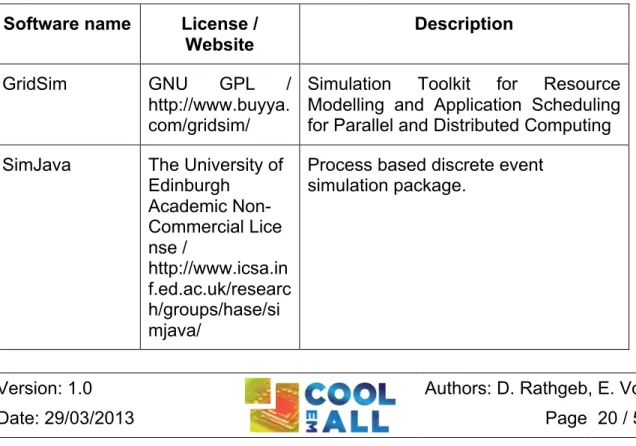
Table 2-6: Software dependency list for DCworms

Software name License / Website

Description GridSim GNU GPL /

http://www.buyya. com/gridsim/

Simulation Toolkit for Resource Modelling and Application Scheduling for Parallel and Distributed Computing SimJava The University of

Edinburgh Academic Non-Commercial Lice nse / http://www.icsa.in f.ed.ac.uk/researc h/groups/hase/si mjava/

Process based discrete event simulation package.

(22)

JFreeChart GNU LGPL / http://www.jfree.o rg/jfreechart/

Java chart library

Castor New Apache-style license / http://castor.code haus.org/

Open Source data binding framework for Java

Apache

Commons Apache License, Version 2.0 / http://commons.a pache.org/

Library focussing on all aspects of reusable Java components

Apache log4j Apache License, Version 2.0 / http://logging.apa che.org/log4j/1.2/

Logging library for Java

Apache Xerces Apache License, Version 2.0 / http://xerces.apac he.org/

Library for parsing, validating and manipulating XML documents.

Joda Time Apache License, Version 2.0 /

http://joda-time.sourceforge. net/

Provides a quality replacement for the Java date and time classes

JUnit Common Public License /

http://junit.sourcef orge.net/

Framework to write repeatable tests

Saxon Mozilla Public License version 2.0,

http://saxon.sourc eforge.net/

(23)

2.2.5 CFD-Solver

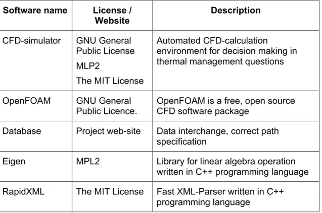
The CFD-Solver does the CFD-simulation and creates the flow field and values on which other components rely on. For its work it needs input from various other components. First it needs the geometry input from the DEBB in .PLMXML-format, retrieved from the DEBB repository. This is then transformed in a simulation region. Additionally there are boundary conditions and initial conditions needed. These values are supplied by the DCworms workload simulator and automatically retrieved from the MOP database. With these starting values the CFD-toolkit performs the flow and temperature simulation automatically. Therefore it first reads the relevant geometry files. These files are then meshed automatically and supplied to the CFD-calculation tool which performs the CFD-calculation automatically. After the simulation has finished links to the flow and temperature field are stored in the central database and mean values for all relevant values, e.g. velocity and temperature for the interesting geometry, which are especially inlet and outlet are created and stored to the database.

To perform these calculations different tools of OpenFOAM and specifically developed software is used. The following table summarizes software used by CFD solver.

Table 2-7: Software dependency list for CFD

Software name License /

Website Description

CFD-simulator GNU General Public License MLP2

The MIT License

Automated CFD-calculation

environment for decision making in thermal management questions

OpenFOAM GNU General Public Licence.

OpenFOAM is a free, open source CFD software package

Database Project web-site Data interchange, correct path specification

Eigen MPL2 Library for linear algebra operation written in C++ programming language RapidXML The MIT License Fast XML-Parser written in C++

(24)

At the beginning the setup of the case is done by a script. Then the simulation environment is set up for blockMesh. This is done by parsing a XML-file and the rest of the setup for blockMesh is then done automatically. BlockMesh then creates a rectangular mesh. This is the basis for the work of snappyHexMesh. But before snappyHexMesh can start its work the .PLMXML-file needs to be parsed and the necessary transformations for the .STL-files, which are the mandatory geometry representations are made. These .STL-files have to be supplied to the toolkit by the user and need to represent all used geometry, especially inlets and outlets, individually. These geometry files are then used by snappyHexMesh to create the computational mesh. After the geometry is transformed into a computational mesh the boundary conditions are set up automatically by invoking the governing scripts and specially developed programs. For all different geometry representations this setup is performed individually. After these introducing steps the decomposition of the mesh is done and the actual calculation is performed in parallel mode to speed up the process. The solver to perform the calculation is bouyantBoussinesqSimpleFoam. It is capable of calculating incompressible flow for stationary conditions in conjunction with heat transfer. After the parallel solver has finished the decomposed computational mesh is reassembled and converted to EnSight and VTK format. EnSight-format is the preferred format for COVISE and VTK is the preferred format for Open Source applications such as ParaView. The next step is to calculate the mean values for the relevant geometry and store the data directly to the database. For the flow fields only links are stored to the database to safe space inside the database. The utility to perform the final calculation is swak4foam and it is invoked automatically by the governing script.

Dependencies exist especially on the input site of the CFD-Solver. Here are to name the geometry files, which have to be .STL-files. These .STL-files need to be references correctly by the .PLMXML-file which represents the DEBB. To ensure consistency between all the invoked applications a naming convention was made.

A second very important convention is set up to find the data stored in the database. This is done by a convention for the data storage path in the database. Another dependency is on the site of the boundary conditions. To create the correct boundary conditions the CFD-solver needs the output of the DCworms workload simulator in the units and for the correct values. The values monitored for this stage power and airflow is used.

For the output only on dependency is obvious. The data which has to be stored to the database needs to be put on the right place. Therefore the path where the input data is located is reused and the according data is added.

As noted, each functional surface, e.g. inlet and outlet has their own .STL-files and need to be referenced in .PLMXML-file. This is necessary for setting up the boundary conditions for CFD-simulation. For this purpose next sections describe naming conventions used in .PLMXML-file and path.

(25)

2.2.5.1 Naming convention for PLMXML-file

For now this convention needs to be applied for the ProductInstances, as these are the parts which matter for the CFD-simulation. This naming convention is used for the name of the ProductInstance, e.g. the name specified in the first line of the product instance.

As pointed out, the generation of the geometry data is extracted from the DEBB (main PLMXLM file), containing references to geometric objects specified in .stl files, as described in D3.2 ([D3.2]). The geometric objects are composed of faces. There are four (4) significant faces for CFD, hat are handled in simulation in different way:

• inlet (source of airflow) • outlet (exhausting airflow) • heatsink (source of heat)

• wall (surface reflecting the airflow)

For specification of the boundary patch, an inlet, name of ProductInstance-Element within the PLMXML file should consist of the keyword, specifying face-type (for inlet this keyword is “inlet”). Next there is a”§” as a separator followed by the name of the corresponding geometry-object the according boundary patch belongs to.

< face-type>§<object-name >

• <face-type> is element of {“inlet”, “outlet”, “heatsink”}, in case of absence of face-type, “wall” face-type is presumed.

• <object-name> is the name of the geometry-object and might contain “@”, that is converted to ‘/’ path-separator used to access object-path. An example for this is: inlet§RackNECWC_01@inlet_01, specifying face-type inlet, object RackNECWC_01 and its part inlet_01.

2.2.5.2 Path to data stored in database

The database stores different input parameters for CFD simulations (such as power and airflow), that belongs to particular surfaces of objects, used within simulation. In order to setup simulation with right parameters (boundary conditions) belonging to corresponding geometry-object, such as airspeed at “inlet” of a rack, these parameters are queried from the database using full object-path to particular geometrical object. The full object-path is built as a concatenation of all object-names in the hierarchy of PLMXML file:

(26)

We always start out with the configuration of whole setup. We start which the name of the server room (level 1), followed by “/”. Next is the name of the rack (level 2), etc. This makes up the path to the important data stored for the CFD. Inside this path there is the necessary data stored:

• Pressure p • Temperature T • Velocity U

Example: HLRSServerroom/RackNECWC_01/inlet_1

2.2.5.3 Orientation of velocity at inlet

The .STL-files used to define the geometry for CFD-simulation input need the following orientation convention.

The tessellation of .STL-file has to be done according to the right-hand-rule. The face normal vector which results from this rule has to point in direction of flow for the inlet.

Table 2-8: Software dependency list for CFD

Software name License / Website

Description CFD-simulator GNU General

Public License MLP2

The MIT License

Automated CFD-calculation

environment for decision making in thermal management questions

OpenFOAM GNU General Public Licence.

OpenFOAM is a free, open source CFD software package

Database Project web-site Data interchange, correct path specification

Eigen MPL2 Library for linear algebra operation written in C++ programming language RapidXML The MIT License Fast XML-Parser written in C++

(27)

2.2.6 Metric Calculator

As described in D2.2, the Metric Calculator is responsible for the assessment of the simulation results. Based on metrics identified and defined in D5.1, it assesses energy-efficiency and heat-efficiency of building blocks (DEBBs). The calculation itself is based on data/metrics that are retrieved from the Database. Results of the calculation are written back into the Database, to be retrieved and visualized by MOP GUI.

The realisation of the Metric Calculator is done by the python command line application that can be called with many different parameters depending of the selected metric calculation.

The Metric Calculator is a python command line application that can be called with many different parameters depending of the calculations performed. The calculation is based on metrics retrieved from the database. The current implementation of metric calculator for 1st_{prototype allows calculating following}

metrics:

Hardware level metrics: • thermal_imbalance

• power_usage (over time range)

• minimum power_usage (over time range) • maximum_power (over time range) • average_power (over time )

• energy

Application level metrics:

• process_energy (for particular task over time-range) • process_temperature (for particular task over time-range)

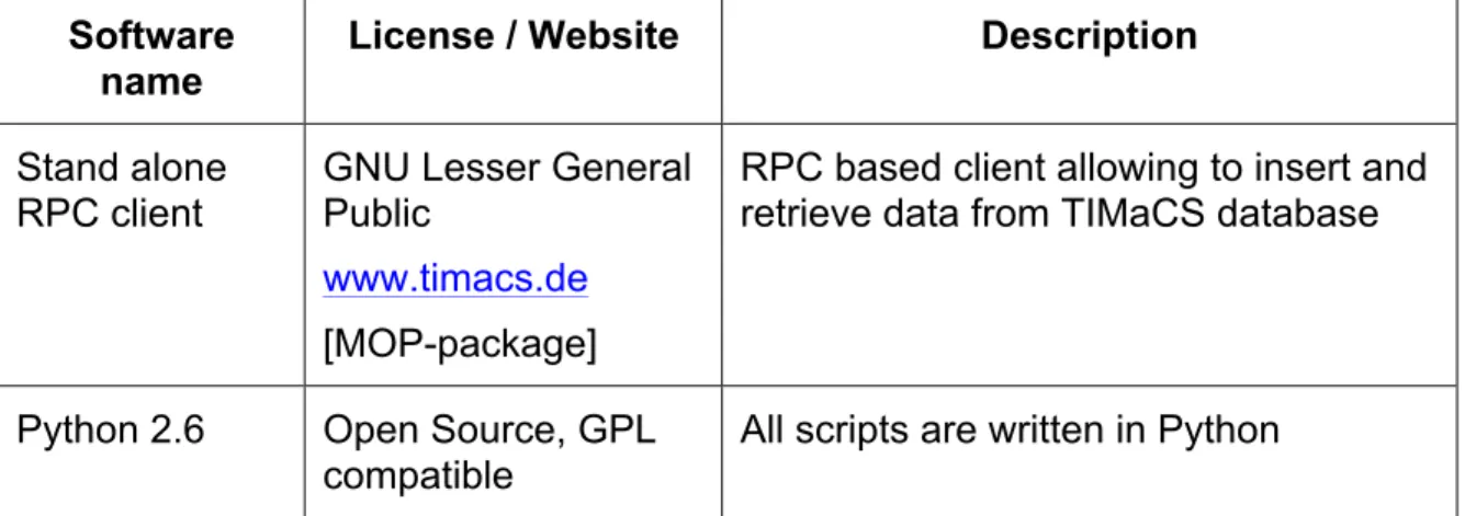
Table 2-9: Software dependency list for Metric Calculator

Software name

License / Website Description Stand alone

RPC client

GNU Lesser General Public

www.timacs.de

[MOP-package]

RPC based client allowing to insert and retrieve data from TIMaCS database

Python 2.6 Open Source, GPL compatible

(28)

(29)

3 Usage of SVD Toolkit components

In this section we describe how SVD Toolkit components are used to enable execution of experiments (simulation).

3.1 Application Profiler

As previously stated, the Application Profiler is quite simple to use. Each time an application is run on the test-bed, the application is run afterwards to produce its profile using monitored information available in TIMaCS. The resulting XML file is stored in the SVN hierarchy following the official CoolEmAll architecture. These files can then be read by DCworms for simulation purpose.

3.2 SVN Repository

As previously state, SVN repository provides access to: application profiles, workload-profiles, DEBBs, and experiment configurations, used by SVD-Toolkit components for execution of experiments/simulations. In order to interact with repository, on the client side, the user runs a Subversion client application - typically a command line client, but possibly a GUI client as well. There exist a number of SVN clients, capable to access SVN server (repository). The most used command line options by SVN clients are:

• svn checkout - to checkout a working directory from the svn server • svn add - to add a new file or directory to repository

• svn update/up – to update local copy with files from SVN server. • svn commit/ci – to recursively sends local changes to the SVN server • svn list – to display files in a directory for any given revision

• svn update – r <revision-number> - to check out specific revision

The usage of repository is done according to structure and conventions described in section 2.2.2.

3.3 Database

The database comprises several methods via RPC that can be called to insert and to retrieve data. To simplify query of the database, we implemented script based API:

• coolemall_getExperimentsList

- Return a list of all the experiments saved on the database.

• coolemall_getLastMetricByMetricName object_path metric_name [experiment_ID trial_ID]

(30)

- Return the last metric specified by metric_name, object_path, experiment_ID and trial_ID. Experiment_ID and trial_ID are optional. The metric contains the last time and value recorded.

• coolemall_getLastMetricsByHostName object_path [experiment_ID trial_ID]

- Return the last metrics of a specified object_path, for a given experiment_ID and trial_ID. Experiment_ID and trial_ID are optional. • coolemall_getMetricNames object_path [experiment_ID trial_ID]

- Return all the metrics saved for a particular object_path on a specified experiment_ID and trial_ID. Experiment_ID and trial_ID are optional. • coolemall_getHostNames [experiment_ID trial_ID]

- Return all object_path for which metrics are saved from a given experiment_ID and trial_ID. Experiment_ID and trial_ID are optional. • coolemall_getRecordsByMetricName object_path metric_name

[experiment_ID trial_ID start_time, end_time]

- Return a list of metrics that contains record objects. Each record has three attributes: time, value and output. The arguments experiment_ID, trial_ID, start_time and end_time are optional. The argument start_s in seconds specifies the earliest record to be returned. No records newer than end_s (in seconds) are returned.

• coolemall_getTrialsList experiment_ID

- Retrieve all trial_ids for a specified experiment_ID • coolemall_putMetricDB “metric_attribute”

- Insert into database the parameters specified in the string by command line. Each attribute is a set of tuples key:value separated by comma (,) that represent the metric. For example:

“experiment_id:id_2,time:139893248,...”

3.4 DCworms

As stated in [D2.2] and presented in 2.1 the input to the workload simulation phase consists of workload and application profiles as well as DEBB model. In general, in DCworms all these information are included within the single configuration file that is passed as an input parameter. This file has a typical, java resource bundle format. List of all available parameters is presented below.

workload=workload.swf

resdesc=serverRoom.xml

debb2dcworms=plugins.xml

workload parameter specifies the path and name of the file containing the workload profile. For the purposes of the workload description within the SVD Toolkit we adopted Standard Workload Format (SWF) [SWF]. In addition to the predefined labels in the header comments, we introduce support of new one that is used to provide information about types of applications used within the given

(31)

set of tasks. In this way, workload profile contains the references to the corresponding application profiles that will be loaded and linked during the simulation. More details of the workload and application profiles and the format of the particular descriptions can be found in [D2.3].

resdesc parameter points the path and name of file with the DEBB description. The format of this file was described in [D3.2].

debb2dcworms parameter defines additional XML file containing information about scheduling policies, energy and application performance models, which are unavailable in DEBB, but necessary from the perspective of DCworms. This file is processed before the workload simulation and merged with DEBB file in order to transform it to the native resource description format supported by the simulator. Example XML file with the additional data is presented below.

It contains the name of the plugins that allow researcher to configure and adapt the simulation framework to the experiment scenario starting from modeling

(32)

application performance, through energy estimations up to implementation of resource management and scheduling policies. With respect to the example above, tasks that come to the system will be scheduled according to the policy provided by the FCFSRB_EnOpt_NodePowMan file. Estimation of power consumption will be based on the methods contained within the CPU_Dynamic_EEP and Node_EEP plugin files for all types of nodes and processors defined within the DEBB, respectively. To estimate the execution time of task, the AppTimeEstimationPlugin plugin will be used.

From the above list, only the specification of workload management plugin is required. In case of lack energy/thermodynamic plugins the default ones will be used. They are based on static definitions of power and air flow states and follow changes in the corresponding values. Default application performance model is based on the linear dependency between execution time and resource speed. The following tables contain the name of the plugins with their short description that are provided within the first release of SVD Toolkit.

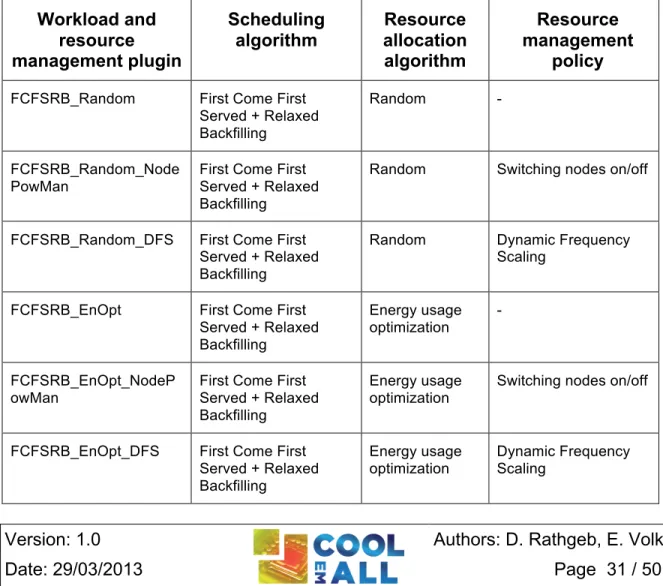
Table 3-1 presents workload and resource management plugins included in DCworms. Their detailed characteristics are provided by [D4.3].

Table 3-1: Workload and resource management plugins/policies available within DCworms

Workload and resource management plugin Scheduling algorithm Resource allocation algorithm Resource management policy

FCFSRB_Random First Come First Served + Relaxed Backfilling

Random -

FCFSRB_Random_Node PowMan

First Come First Served + Relaxed Backfilling

Random Switching nodes on/off

FCFSRB_Random_DFS First Come First Served + Relaxed Backfilling

Random Dynamic Frequency Scaling

FCFSRB_EnOpt First Come First Served + Relaxed Backfilling Energy usage optimization - FCFSRB_EnOpt_NodeP owMan

First Come First Served + Relaxed Backfilling

Energy usage optimization

Switching nodes on/off

FCFSRB_EnOpt_DFS First Come First Served + Relaxed Backfilling Energy usage optimization Dynamic Frequency Scaling

(33)

LJFRB_LoadBal Largest Job First + Relaxed Backfilling

Load Balancing -

LJFRB_LoadBal_NodePo wMan

Largest Job First + Relaxed Backfilling

Load Balancing Switching nodes on/off

LJFRB_LoadBal_DFS Largest Job First + Relaxed Backfilling

Load Balancing Dynamic Frequency Scaling

LJFRB_Consolidation Largest Job First + Relaxed Backfilling

Consolidation -

LJFRB_Consolidation_No dePowMan

Consolidation Switching nodes on/off

LJFRB_Consolidation_D FS

Consolidation Dynamic Frequency Scaling

Table 3-2 shows plugins that are used to perform calculations related to power consumption and air flow estimations. The general idea behind the plugins and implemented models can be found in [D2.2].

Table 3-2: Energy and thermal plugins available within DCworms

Energy and thermodynamic

plugin

Power estimation Air flow estimation

CPU_Static_EEP Based on changes of processor power states

-

CPU_Dynamic_EEP Based on processor load - CPU_App_EEP Based on power required for

executing various types of applications

-

Node_EEP Based on power consumption of all subcomponents

Based on changes of air flow states defined within the DEBB ComputeBox1_EEP Based on power consumption of all

subcomponents

-

(34)

Table 3-3: Application performance plugins available within DCworms

Application

performance plugin Characteristic

BasicTimeEstimationPlugin Calculations of time required to execute the task are based on the assumption that processing time is a linear function of number of allocated processors and their speed.

AppTimeEstimationPlugin Calculations of time required to execute the task are based on the application profiles and their performance models. This plugin follows detailed application characteristics and performs calculations using transformation function between the

execution time on the reference hardware and the current one.

To perform experiments using DCworms user needs to execute the following command, passing the path to the configuration file as a program argument: sbatch --partition=aux runDCworms.sh

experiment1/RECSexperiment1.properties

The simulation is controlled by the testbed queuing system (SLURM) and it is requested to be started on aux partition. The partition is designed for running computations outside the main monitored part of the testbed to not influence the measurements. It consists of two worker nodes that have their own dedicated power lines and are physically separated from rest of the testbed.

3.5 CFD

For this first prototype the interaction with the CFD-solution is done via a command line based script.

Before the invoking of the script can be done a simulation environment needs to be set up. This consists foremost of a working installation of OpenFOAM and a setup of OpenMPI. This is supposed to be done before you start with the setup of the bespoke CFD-solution.

For setting up an automated simulation based on this first prototype it is most convenient to do so in a dedicated directory. In our case this directory is called “auto_OpenFOAM”. In this working directory it is supposed to have the following subdirectories set up: One directory should be called “DEBB”. In this directory the governing .PLMXML-file and the geometry representing .STL-files are stored. Then there is another important directory which is called “control_files”. This directory is particularly important when it is of interest to run several different simulations. In this directory simulation independent solver parameter are stored. These variables are editable but it is not necessary and not recommended to do so. These variables are reused for each independent simulation and therefore these variables are copied to the corresponding files of the simulation case.

(35)

Another important directory is called “TIMaCS”. In this directory are the scripts for invoking the database for automatic creation of boundary and initial conditions stored, as well as the scripts for putting back the simulation results to the database. Then there is directory called “SRC”. In this directory the source code and the executables for the automated setup of the simulation case is stored. So there should be no necessity for the user to interact with this directory.

Then there are some more .TXT and .XML-files. These files are described in the order they are invoked by the setup script. First there is a file called Definition_Quader.xml. In this file the definitions are made for invoking blockMesh. blockMesh sets up the surrounding region in which the geometry to simulate is meshed. Here it is necessary to make sure that the geometry fits into the surrounding region created by blockMesh and therefore the size of this region can be adjusted accordingly in this file called “Definition_Quader.xml. Next the user finds a file called locationInMesh.txt. This file is important for snappyHexMesh. To enable snappyHexMesh to automatically create a mesh based on the region created by blockMesh and the .STL-files transformed by the PLMXML-parser it is necessary to specify a point inside the mesh, in a region where the mesh should be kept. The point inside the mesh region to keep is stated in the file called “locationInMesh.txt”

In the file called temperature.txt temperature values for boundaries which are not referenced in the database are stored. This is necessary as there are no temperature sensors available on these boundaries, which are for example sidewalls. These values should be submitted in degrees Celsius in the format found in the file and are editable by the user.

After a simulation was done a new directory called “case1” appears. In this directory the data for the whole simulation can be found. And this directory is deleted and remade every time a simulation is started automatically. So if the user desires to keep the whole simulation case it is best to move this directory to a different location before another automatic simulation is started.

When all this setup is complete, the simulation can be started automatically just by calling the script called Autorun with submitting the path to the location on the .PLMXML-file and the name of the host for which the metrics are stored. The retrieving of all relevant data and the calculation is then performed automatically.

3.6 Metric Calculator

The Metric Calculator is a python command line application that can be called with many different parameters depending of the calculation.

Measurements and calculations can be done at two levels. The hardware level where most data are measured, aggregated or calculated (calculations are based on real measurements) and the application level where most of the data are estimated and calculated (calculation are based on estimations)

(36)

3.6.1 Hardware level metrics:

In this section we describe hardware level metrics.

./metricCalc.py imbalance_of_temperature <path> <start_s> <end_s>

Calculate the thermal imbalance of the hardware element “path” (CPU, recs, rack, datacenter) between the given start and end time.

The resulting metric will be stored at “path” level with the timestamp end_s and the name:

ImbalanceOfTemperature-From:start_s-To:end_s

. ./metricCalc.py power <path> <start_s> <end_s>

Calculate the power of the hardware element “path” (recs, rack, datacenter) for each timestamp between the given start and end time.

The resulting metric will be stored at “path” level with the name:

Power

./metricCalc.py minimum_power <path> <start_s> <end_s>

Calculate the minimum power of the hardware element “path” (recs, rack, datacenter) over a period of time.

MinPower-From:start_s-To:end_s

./metricCalc.py maximum_power <path> <start_s> <end_s>

Calculate the maximum power of the hardware element “path” (recs, rack, datacenter) over a period of time.

MaxPower-From:start_s-To:end_s

./metricCalc.py average_power <path> <start_s> <end_s>

Calculate the average power of the hardware element “path” (recs, rack, datacenter) over a period of time.

(37)

./metricCalc.py energy <path> <start_s> <end_s>

Calculate the energy consumption of the hardware element “path” (recs, rack, datacenter) over a period of time.

Energy-From:start_s-To:end_s

3.6.2 Application level metrics

In this section we describe application level metrics.

./metricCalc.py process_energy <pid or Slurm task ID path> [<start_s> <end_s>]

Calculate the energy consumption of the process (or each process of the task) at the given path for each timestamp over the full process lifetime (or a defined period of time).

The resulting metric will be stored at process level with the name: Energy (calculation over process lifetime)

Or Energy-From:start_s-To:end_s (calculation over a specific interval) ./metricCalc.py process_temperature <pid or Slurm task ID path> [<start_s> <end_s>]

Calculate the temperature of the process (or each process of the task) at the given path for each timestamp over the full process lifetime (or a defined period of time).

The resulting metric will be stored at process level with the name: Temperature (calculation over process lifetime),

Or Temperature-From:start_s-To:end_s (calculation over specific interval)

4 Test of SVD Toolkit components

In this section we describe tests of SVD Toolkit components, including Application profiler, Repository, Database, Data Centre workload simulator, CFD solver and metric calculator.

(38)

4.1 Application Profiler

Test of the application profiler has been done by creating the profile of one the HPC benchmark EP with different frequencies. The faster the processor, the least number of phases are detected as some slight behaviour changes do not have enough impact at faster speed to be detected as new phases.

Profile at fastest speed

<resourceConsumptionProfile> <resourceConsumption> <referenceHardware>Intel_i7</referenceHardware> <duration>PT4S</duration> <behaviour name="cpu"> <value>99</value> </behaviour> <behaviour name="network"> <value>29</value> </behaviour> </resourceConsumption> <resourceConsumption> <referenceHardware>Intel_i7</referenceHardware> <duration>PT67S</duration> <behaviour name="cpu"> <value>98</value> </behaviour> <behaviour name="network"> <value>88</value> </behaviour> </resourceConsumption> <resourceConsumption> <referenceHardware>Intel_i7</referenceHardware> <duration>PT8S</duration> <behaviour name="cpu"> <value>98</value> </behaviour> <behaviour name="network"> <value>29</value> </behaviour> </resourceConsumption> <resourceConsumption> <referenceHardware>Intel_i7</referenceHardware> <duration>PT63S</duration> <behaviour name="cpu"> <value>98</value> </behaviour> <behaviour name="network"> <value>85</value> </behaviour> </resourceConsumption> <resourceConsumption> <referenceHardware>Intel_i7</referenceHardware> <duration>PT69S</duration> <behaviour name="cpu"> <value>98</value> </behaviour> <behaviour name="network"> <value>85</value> </behaviour> </resourceConsumption> <resourceConsumption> <referenceHardware>Intel_i7</referenceHardware> <duration>PT61S</duration> <behaviour name="cpu"> <value>98</value> </behaviour> <behaviour name="network"> <value>80</value> </behaviour> </resourceConsumption> <resourceConsumption> <referenceHardware>Intel_i7</referenceHardware> <duration>PT72S</duration> <behaviour name="cpu"> <value>98</value> </behaviour> <behaviour name="network"> <value>76</value> </behaviour> </resourceConsumption> </resourceConsumptionProfile>

Profile at slowest speed

<resourceConsumptionProfile> <resourceConsumption> <referenceHardware>Intel_i7</referenceHardware> <duration>PT4S</duration> <behaviour name="cpu"> <value>99</value> </behaviour> <behaviour name="network"> <value>28</value> </behaviour> </resourceConsumption> <resourceConsumption> <referenceHardware>Intel_i7</referenceHardware> <duration>PT46S</duration> <behaviour name="cpu"> <value>98</value> </behaviour> <behaviour name="network"> <value>92</value> </behaviour> </resourceConsumption> <resourceConsumption> <referenceHardware>Intel_i7</referenceHardware> <duration>PT18S</duration> <behaviour name="cpu"> <value>98</value> </behaviour> <behaviour name="network"> <value>38</value> </behaviour> </resourceConsumption> <resourceConsumption> <referenceHardware>Intel_i7</referenceHardware> <duration>PT72S</duration> <behaviour name="cpu"> <value>98</value> </behaviour> <behaviour name="network"> <value>90</value> </behaviour> </resourceConsumption> <resourceConsumption> <referenceHardware>Intel_i7</referenceHardware> <duration>PT12S</duration> <behaviour name="cpu"> <value>98</value> </behaviour> <behaviour name="network"> <value>40</value> </behaviour> </resourceConsumption> <resourceConsumption> <referenceHardware>Intel_i7</referenceHardware> <duration>PT72S</duration> <behaviour name="cpu"> <value>98</value> </behaviour> <behaviour name="network"> <value>90</value> </behaviour> </resourceConsumption> <resourceConsumption> <referenceHardware>Intel_i7</referenceHardware> <duration>PT4S</duration> <behaviour name="cpu"> <value>98</value> </behaviour> <behaviour name="network"> <value>44</value> </behaviour> </resourceConsumption> <resourceConsumption> <referenceHardware>Intel_i7</referenceHardware>

(39)

(40)

Version: 1.0 Authors: D. Rathgeb, E.Volk

4.2 SVN Repository

As noted, the interaction with SVN repository is done via svn-client (svn command). The following example shows interaction with the svn:

volk@timacs:~/coolemall-repository$ svn co https://svn.coolemall.eu/svn/repository A repository/users A repository/common A repository/common/debbs A repository/common/workloads A repository/common/applications Checked out revision 51.

volk@timacs:~/coolemall-repository$ cd common/

volk@timacs:~/coolemall-repository/repository/common$ ls applications debbs workloads

volk@timacs:~/coolemall-repository/repository/common$ mkdir experiments volk@timacs:~/coolemall-repository/repository/common$ ls

applications debbs experiments workloads

volk@timacs:~/coolemall-repository/repository/common$ svn ci Adding common/experiments

Committed revision 52.

volk@timacs:~/coolemall-repository/repository/common$

4.3 Database

To execute the python wrapper it needed start the coolemalldb demon: [timacs@recs1 coolemall] ./bin/coolemall

usage: coolemall <option>

-h|--help This blurb.

-k|--kill|--stop Stop coolemalldb. -s|--start Start coolemalldb.

-i|--status Show status of coolemalldb. Example invocation:

(41)

Version: 1.0 Authors: D. Rathgeb, E.Volk coolemall --start

The test of the collemall DB using script based API (described in Section 3.3) are show below:

[timacs@recs1 coolemall]$ ./coolemall_getRecordsByMetricName testbed/hlrs/hpc/hw/rack1/recs1/i7_0_05 mem_usage

[(1361574545L, 42356.230000000003, 'ok-low')]

[timacs@recs1 coolemall]$ ./coolemall_getMetricNames testbed/hlrs/hpc/hw/rack1/recs1/i7_0_05

[cpu_usage, mem_usage, usr_load]

[timacs@recs1 coolemall]$ ./coolemall_getHostNames

[testbed/hlrs/hpc/hw/rack1/recs1/i7_0_05, testbed/hlrs/hpc/hw/rack1/recs1, testbed/hlrs/hpc/hw/rack1]

[timacs@recs1 coolemall]$ ./coolemall_getLastMetricsByHostName testbed/hlrs/hpc/hw/rack1/recs1/i7_0_05

[Metric(name='cpu_usage', output='ok-low', value=6.21, source='nagios', host='testbed/hlrs/hpc/hw/rack1/recs1/i7_0_05', time=1361574550L, performance='ok-2.5'), Metric(name='mem_usage', output='ok-low',

value=42356.230000000003, source='nagios',

host='testbed/hlrs/hpc/hw/rack1/recs1/i7_0_05', time=1361574545L, performance='ok-1.5'), Metric(name='usr_load', output='ok-low',

value=12.210000000000001, source='nagios',

host='testbed/hlrs/hpc/hw/rack1/recs1/i7_0_05', time=1361574525L, performance='ok-2.5')]

[timacs@recs1 coolemall]$ ./coolemall_getLastMetricByMetricName testbed/hlrs/hpc/hw/rack1/recs1/i7_0_05 cpu_usage host = testbed/hlrs/hpc/hw/rack1/recs1/i7_0_05 name = cpu_usage output = ok-low performance = ok-2.5 source = nagios