HAL Id: lirmm-00415780
https://hal-lirmm.ccsd.cnrs.fr/lirmm-00415780
Submitted on 10 Sep 2009HAL is a multi-disciplinary open access
archive for the deposit and dissemination of sci-entific research documents, whether they are pub-lished or not. The documents may come from teaching and research institutions in France or
L’archive ouverte pluridisciplinaire HAL, est destinée au dépôt et à la diffusion de documents scientifiques de niveau recherche, publiés ou non, émanant des établissements d’enseignement et de recherche français ou étrangers, des laboratoires
coniferous forest: assessing terrain and tree height
quality
Adrien Chauve, Cedric Vega, Sylvie Durrieu, Frédéric Bretar, Tristan Allouis,
Marc Pierrot-Deseilligny, William Puech
To cite this version:
Adrien Chauve, Cedric Vega, Sylvie Durrieu, Frédéric Bretar, Tristan Allouis, et al.. Process-ing full-waveform lidar data in an alpine coniferous forest: assessProcess-ing terrain and tree height qual-ity. International Journal of Remote Sensing, Taylor & Francis, 2009, 30 (19), pp.5211-5228. �10.1080/01431160903023009�. �lirmm-00415780�
For Peer Review Only
Advanced full-waveform lidar data echo detection: assessing quality of derived terrain and tree height models in an alpine coniferous forest
Journal: International Journal of Remote Sensing Manuscript ID: TRES-SIP-2008-0022.R1
Manuscript Type: Special Issue Paper Date Submitted by the
Author: n/a
Complete List of Authors: Chauve, Adrien; Institut Géographique National, Laboratoire MATIS; CEMAGREF, UMR TETIS; LIRMM, Université Montpellier II Vega, Cédric; CEMAGREF, UMR TETIS
DURRIEU, Sylvie; CEMAGREF, UMR TETIS
Bretar, Frédéric; Institut Géographique National, Laboratoire MATIS Allouis, Tristan; CEMAGREF, UMR TETIS
Pierrot Deseilligny, Marc; CEMAGREF, UMR TETIS Puech, William; LIRMM, Université Montpellier II Keywords: DIGITAL ELEVATION MODEL, LIDAR, MODELLING
Keywords (user defined): FOREST, WAVEFORM ANALYSIS, TREE HEIGHT MEASUREMENTS
For Peer Review Only
International Journal of Remote Sensing Vol. 00, No. 00, DD Month 200x, 1–26
Special Issue Paper
Advanced full-waveform lidar data echo detection: assessing quality of derived terrain and tree height models in an alpine
coniferous forest
A. CHAUVE∗ † ‡ §, C. VEGA†, S. DURRIEU†, F. BRETAR‡, T. ALLOUIS†, M.
PIERROT DESEILLIGNY† and W. PUECH§
†UMR TETIS Cemagref/Cirad/ENGREF-AgroParisTech, Maison de la T´el´ed´etection,
34093 Montpellier Cedex 5, France
‡ Laboratoire MATIS - Institut G´eographique National, 2-4 Avenue Pasteur, 94165 Saint
Mand´e cedex, France
§ Laboratoire LIRMM, UMR CNRS 5506, Universit´e Montpellier II
161, rue Ada, 34392 Montpellier Cedex 05, France
(Received 00 Month 200x; in final form 00 Month 200x)
Small footprint full-waveform airborne lidar systems hold large opportunities for improved forest characterisation. To take advantage of full-waveform information, this paper presents a new processing method based on the decomposition of waveforms into a sum of parametric functions. The method consists of an enhanced peak detection algorithm combined with an advanced echo modelling including Gaussian and generalized Gaussian models. The study focussed on the qualification of the extracted geometric information. Resulting 3D point clouds were compared to the point cloud provided by the operator. 40 to 60 % additional points were detected mainly in the lower part of the canopy and in the low vegetation. Their contribution to Digital Terrain Models (DTMs), Canopy Height Models (CHMs) was then analysed. The quality of DTMs and CHM-based heights was assessed using field measurements on black pine plots under various topographic and stand characteristics. Results showed only slight improvements, up to 5 cm bias and standard deviation reduction. However both tree crowns and undergrowth were more densely sampled thanks to the detection of weak and overlapping echoes, opening up opportunities to study the detailed structure of forest stands.
Keywords: LIDAR, FOREST, WAVEFORM ANALYSIS, MODELLING, DIGITAL EL-EVATION MODEL, TREE HEIGHT MEASUREMENTS
∗Corresponding author. Email: [email protected]
International Journal of Remote Sensing 1 2 3 4 5 6 7 8 9 10 11 12 13 14 15 16 17 18 19 20 21 22 23 24 25 26 27 28 29 30 31 32 33 34 35 36 37 38 39 40 41 42 43 44 45 46 47 48 49 50 51 52 53 54 55 56 57 58 59 60
For Peer Review Only
1. Introduction
Trends in forest inventory and management go towards the acquisition of automatic, spatially explicit, and repeatable information on forest structure and function. During the last decade, airborne laser scanning altimetry or small-footprint lidar (light detection and ranging) proved to be the most suitable remote sensing technique to map simultaneously both forest attributes and the ground topography.
Current systems can record up to six returns by emitted pulse. First intercep-tions of the signal generating first returns describe the shape of objects on the earth surface visible from above, and can be used to produce a digital surface model (DSM). The DSM quality depends mainly on the interpolator used and the selected grid resolution (Vepakomma et al. 2008). The last returns describe the furthest surfaces interacting significantly with the laser beam including ground re-turns. They are individually classified into ground and non-ground categories using geometrical rules (Sithole and Vosselman 2004, Axelsson 1999) to produce a digital terrain model (DTM) representing the ground topography. The ground elevation errors in lidar DTMs are usually less than 30 cm under a forest cover (Hodgson and Bresnahan 2004, Reutebuch et al. 2003, Ahokas et al. 2003). However, most of the current algorithms rely on local calibration providing suboptimal results in heterogeneous terrain. This is explained by errors induced by both a decrease in the signal to noise ratio of the backscatter and the effect of slope (see Kobler et al. (2007) for a review on lidar filtering). Improving the precision and accuracy of DTMs under varying topographical conditions requires the development of robust methods with low sensitivity to the calibration settings (Bretar and Chehata 2008). In forested environments, subtracting the DTM from the DSM produces a canopy height model (CHM) representing the top-of-canopy topography. Such in-formation has been widely used to extract forest parameters at various scales. Using very dense lidar sampling, individual tree height can be measured with a root mean square error (RMSE) of about 1 meter (Persson et al. 2002, Andersen et al. 2001). At the stand level, mean tree height errors of 2.0m or less were reported (Hollaus et al. 2006, Naesset 1997). Based on vertical point distribution, additional forest parameters were also successfully estimated such as crown size, basal area, stem density, volume, and biomass (see Lim et al. (2003) for review). As for ground topography, current researches focus on estimating robust or universal lidar indi-cators of forest parameters (Hopkinson et al. 2006).
Most of the studies have shown that lidar data underestimate total tree heights (Anderson et al. 2006). These underestimations can be first explained by sampling problems, a small proportion of laser pulses interacting with the tree apices (Mag-nussen and Boudewyn 1998). Consequently acquiring very dense point clouds was recommended to describe the crown characteristics accurately, including total tree height (Hyyppa et al. 2001). A recent study demonstrated that an other source of underestimation relies on the fact that laser pulses slightly penetrate into the foliage before a return could be recorded due to both canopy structural characteristics and lidar device configuration (Gaveau and Hill 2003).
Recent developments of full-waveform lidar systems provide data allowing more control and flexibility on point extraction processes, thus improving measurements reliability. These systems digitize and record the entire backscattered signal of each emitted pulse (see figure 1). Experimental systems with large footprint developed by NASA (Blair et al. 1999) have been successfully used in forest environments for measuring canopy height (Lefsky et al. 1999) or the vertical distribution of canopy
1 2 3 4 5 6 7 8 9 10 11 12 13 14 15 16 17 18 19 20 21 22 23 24 25 26 27 28 29 30 31 32 33 34 35 36 37 38 39 40 41 42 43 44 45 46 47 48 49 50 51 52 53 54 55 56 57 58 59 60
For Peer Review Only
material (Dubayah et al. 2000).
In forest environments, new commercial small-footprint full-waveform systems allowthe recording of detailed information about the geometric and physical properties of the backscattering objects (Reitberger et al. 2006). Processing wave-forms had already proved efficient in increasing the number of detected targets in comparison with data provided by multi-echo lidar systems. Furthermore, the information on how points are extracted in traditional multi-echo lidar systems is generally not given to users by the data provider (Persson et al. 2005). This is particularly tricky in complex forested areas where waveforms can be composed of weak returns from the top of canopy or from the ground, and also of groups of overlapping echoes originated from distributed backscatters in-side the different layers of the vegetation. Traditional threshold-based multi-echo detection algorithms are not suitable to detect or separate such very low peaks or groups of echoes (see figure 1). Therefore, waveform processing aims at improving point extraction and recording additional target information from the waveform shape.
Different methods have been proposed forecho detection(e.g. threshold, zero crossing, local maxima, see Wagner et al. (2004) for review and discussion). One of the more efficient and widespread method consists in decomposing the waveform into a sum of parametric functions, where each function models the contribution of a target to the backscattered signal (Wagner et al. 2004). It was demonstrated that lidar waveforms could be generally well modelled by a sum of Gaussian pulses (Wagner et al. 2006). Non-linear least squares (NLS) methods (Hofton et al. 2000), Gauss-Newton (Jutzi and Stilla 2005) or maximum likelihood estimation using the Expectation Maximization (EM) algorithm (Persson et al. 2005) were used to fit the model to the waveforms. However Gaussian models assume that the pulse has a Gaussian shape and targets are Gaussianscatterers. The latter assumption is not always true (Steinvall 2000).
In this paper, we propose a new method to process the waveforms and investigate the usefulness of non Gaussian parametric models such as generalized Gaussian model to deal with non Gaussian echoes. Such models are expected to improve the point extraction process in forested environments. The extracted point clouds are compared with the point cloud computed from basic signal processing provided by the lidar operator. Further analyses are conducted to quantify the potential of such data to derive precise DTM and CHM-based total tree height measurements.
2. Study site and data sets
2.1 Study site
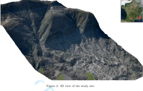
The study area is located in southern French Alps in the neighbourhood of Digne-les-Bains (Alpes-de-Haute-Provence, 04) in the Haute-Bl´eone state forest. This 108 ha protective afforestation is mainly composed of black pine (Pinus nigra ssp. nigra [Arn.]) originating from the end of the XIXth century. Most of the stands are even-aged and mature. The study area is part of an Observatory for Research on the Environment (ORE Draix) monitoring erosion and hydrological processes in mountainous areas. Elevation ranges from 802 m to 1263 m. The steep topography has a 53 % mean slope reaching up to 100 % locally. Stand density varies from low-densities (100 stems/ha) originating from seed cuttings in the low-lying part of the study site to high densities(more than 750 stems/ha, see table 1). 1 2 3 4 5 6 7 8 9 10 11 12 13 14 15 16 17 18 19 20 21 22 23 24 25 26 27 28 29 30 31 32 33 34 35 36 37 38 39 40 41 42 43 44 45 46 47 48 49 50 51 52 53 54 55 56 57 58 59 60
For Peer Review Only
2.2 Field data
Field inventory data were collected with a differential GPS and a total station during December 2007 on circular plots of 9 m (6 plots) and 15 m (10 plots) radius according to the stand density. Within each plot, the precise tree position, and the following tree characteristics were measured for all the trees with diameter at breast height (dbh) greater than 7 cm: dbh, total and timber heights, crown base height (of lowest living branch of the crown). For two of these plots, the crown diameters were also measured. To validate lidar derived DTMs, terrain elevation measurements were collected for four plots characterised by different topographic conditions. For each plot, 64 to 84 measurements were collected using a sampling pattern as regular as possible.
The accurate position of plot centres was measured using a Leica total station within a centimetric precision. The individual tree positions were derived from distance and angle measurements from the plot centre. Distance measurements were taken at the tree base using a Vertex III clinometer (Hagl¨off, Sweden) with slope compensation. Azimuths were measured with a Suunto compass.
Tree heights and crown base heights were collected with the same clinometer instrument. Crown diameters were measured from the trunk in the four cardinal directions using a tape measure. The dbh was measured using a tape measure within a centimetric precision.
For the purpose of that study, we focused the analysis on 4 plots described by both vegetation and topographic measurements. These plots are characterised by different topographic conditions and tree density classes. Table 1 summarizes the plot characteristics.
2.3 Lidar data sets
The data acquisition was performed in April 2007 using a RIEGL c LMS-Q560 system. This sensor is a small-footprint airborne laser scanner. Its main technical characteristics is presented in Wagner et al. (2006). The lidar system operated at a pulse rate of 111 kHz. The flight height was approximatively 600 m leading to a footprint size of about 0.25 m. The point density was about 5 pts/m2.
Two different data sets were provided by the lidar operator: georeferenced 3D point clouds obtained by basic processing (hereafter referred to as BP) and full-waveform raw data. BP was carried out using RiANALYZE c Software
(RIEGL c , Austria) and consists of a simple thresholding method for
the peak detection followed by a Gaussian pulse estimation.
Full-waveform raw data consists of 1D intensity profiles along the line of sight of the lidar device. The temporal sampling of the system is 1ns. Each return waveform was made of one or two sequences of 80 samples corresponding to 12 or 24 m length profiles. For each profile, a record of the emitted laser pulse was also provided.
3. Methods
3.1 Waveform processing
The objective of waveform processing is to extract more information on forest structure from raw lidar data than provided by multi-echo lidar systemsor basic
processing methods. To that end, we developed an enhanced peak detection
algorithm to assess the maximum number of relevant echoes in the signal, and to estimate the parameters of the respective models. This algorithm is an 1 2 3 4 5 6 7 8 9 10 11 12 13 14 15 16 17 18 19 20 21 22 23 24 25 26 27 28 29 30 31 32 33 34 35 36 37 38 39 40 41 42 43 44 45 46 47 48 49 50 51 52 53 54 55 56 57 58 59 60
For Peer Review Only
improved version of the method presented in Chauve et al. (2007) dealing with the so-called “ringing effect” which was not considered in the first version. This effect is a small secondary maximum after the emitted pulse due to the hardware waveform recording chain, and can lead to false peak detection on high reflective surfaces. This method is hereafter referred to as advanced processing (AP). The major differences between BP method and our processings (AP) are the initial peak detection step and the iteration of the procedure to find very low peaks and/or peaks in groups of overlapping echoes.
Waveforms (see figure 3) are composed of uniformly-spaced samples {(xi, yi)}i=1,..,n and can be decomposed into a sum of echoes such as
yi = f (xi) = n
X
j=1
fj(xi) (1)
where n is the number of components and fj the model of the jth echo.
The choice of modelling functions to process the waveforms relies on several criteria. First, the function parameters have to be related to the shape and the optical properties of the target. Second, the derivative of the function should have an explicit formulation, in order to use classical curve-fitting algorithms.
3.1.1 Modelling functions. As waveforms used in this study were collected
with a small-footprint lidar, each laser output pulse shape is assumed to be Gaus-sian with a specific and calibrated width. The recorded waveforms are therefore a convolution between this Gaussian distribution and a “surface” function, de-pending on the hit objects. It was thus demonstrated that more than 98% of the observed waveforms with the RIEGL system could be correctly fitted with a sum of Gaussian functions (Wagner et al. 2006). A Gaussian model (hereafter referred to as GA) can be written as
fj,G(x) = Ajexp −
(x − µj)2
2σj2 !
(2)
where Aj is the pulse amplitude, σj its width, and µj the function mode of the jth
echo.
Nevertheless, the backscattered signal is not always Gaussian. Moreover, in
com-plexenvironments such as forested areas, most of the return waveforms are
ac-tually subject to the mixed effects of geometric (e.g. ground slopes, canopy shapes, foliage densities) and radiometric object properties (e.g. the reflectances depends on the species, foliage, branches, ground).
Using more generic models such as the generalized Gaussian model (hereafter referred to as GG) is expected to improve complex waveforms fitting and model flattened or peaked echoes.
The GG model has the following analytical expression:
fj,GG(x) = Ajexp − |x − µj|α 2 j 2σ2 j ! (3)
where Aj is the pulse amplitude, σj its width, µj the function mode and αj the
1 2 3 4 5 6 7 8 9 10 11 12 13 14 15 16 17 18 19 20 21 22 23 24 25 26 27 28 29 30 31 32 33 34 35 36 37 38 39 40 41 42 43 44 45 46 47 48 49 50 51 52 53 54 55 56 57 58 59 60
For Peer Review Only
shape parameter which allows to simulate Gaussian (α =√2), flattened (α >√2) or peaked (α <√2) pulses.
3.1.2 Enhanced peak detection. The enhanced peak detection is an iterative
process based on a Non-Linear Least Squares (NLS) fitting technique (Levenberg-Marquardt algorithm) of the chosen parametric model on the waveform (Chauve et al. 2007). The fitting parameter θ∗ is computed as:
θ∗ = argmin n X i=1 (yi− f (xi|θ))2 ! (4)
with the quality of the fit ξ evaluated by
ξ(θ∗) = 1 n − dimθ∗ n X i=1 (yi− f (xi|θ∗))2 (5)
The first step of the algorithm is a coarse peak detection, based on zero-crossings of the signal’s first derivative. It allows to estimate the number and the position of the echoes in order to initialize the NLS fitting. In a second step, additional peaks are searched in the difference between modelled and raw signals. If new peaks are found, the fit is performed again and its quality re-evaluated. The process is iterated until no further improvement is obtained. The selected solution is the model providing the minimum value for equation (5).
The main sources of ill detection are: the background noise, and the
ring-ing effect.To take them into account the following rules are appliedto the signal: 1) the noise is thresholded at a mean plus standard deviation level, 2) only one peak is kept when two very close echoes are detected under the lidar system resolution, which reduces overfitting that may result from the
optimiza-tion criterion used ξ (see equaoptimiza-tion 5) and 3) the peaks due to the ringing
effect are removed based on an amplitude ratio criterion.
In the following steps, only the geometric information (e.g. the 3D point cloud) is used to calculate total tree height based on DTM and CHM which are the most commonly used models in lidar-based forest inventory.
3.2 Computation of Digital Models
Digital Terrain Model: Processing airborne lidar data to compute DTMs is a
challenging task, especially in case of alpinerelief with steep slopes.
The methodology used to compute DTMs has been fully developed in(Bretar
and Chehata 2008). It is based on a two-step process: 1) the computation of an
initial surface using a predictive Kalman filter and 2) the refinement of this surface using a Markovian regularization.
The first step aims at providing a robust surface containing low spatial frequen-cies of the terrain while the second step aims at integrating microrelief within the surface to refine the terrain description. The Kalman filter estimates the terrain surface by locally analysing the point cloud distribution composed of first and last echoes in the frame of the local slope. Lidar points considered as ground points (at a defined height of the initial surface) are then included in the regularization step to generate a refined DTM. 1 2 3 4 5 6 7 8 9 10 11 12 13 14 15 16 17 18 19 20 21 22 23 24 25 26 27 28 29 30 31 32 33 34 35 36 37 38 39 40 41 42 43 44 45 46 47 48 49 50 51 52 53 54 55 56 57 58 59 60
For Peer Review Only
Canopy Height Model: A canopy height model (CHM) was obtained by 1)
inter-polating the first returns into a digital surface model (DSM) and 2) subtracting the DTMfromthe DSM. The CHM quality depends mainly on the interpolator used and the selected grid resolution (Vepakomma et al. 2008). In forested environments over mountainous terrain, it was suggested that Universal Kriging might be the most adapted method for deriving DSMs(Lloyd and Atkinson 2002). However IDW (Inverse Distance Weighted) has also been recommended for lidar data with a small point spacing under various topographical conditions (Vepakomma et al. 2008, Anderson et al. 2005). IDW also allows faster computation compared with Kriging methods.
The visual inspection of the point cloud reveals significant disparities in the point density mostly according to the vegetation structure. Local density is quite constant on bare earth, increases on the exposed side of the tree crowns and is minimal on the opposite or shadowed parts of the crowns. As only a small overlap was set between flight lines, the point density remains largely variable in a given neighbourhood. To deal with such varying point patterns, different gridding methods (IDW, Universal Kriging, TIN, neighbourhood statistics using a maximum criterion) were tested. Results of this preliminary work revealed that combining neighbourhood statistics (maximum point value within a given cell) with an interpolation based on IDW for empty cells was best suited for tree height measurements. Thelatter method was used to compute the final CHM at 50 cm resolution according to the average point spacing.
3.3 Statistical analysis
Statistical analyses were performed on four field validation plots having data for both ground elevation and vegetation structure.
3D point clouds extracted from advanced waveform processing were directly compared to the one provided by the lidar operator. First the total number of detected echoes, the ratio of waveforms providing at least one point and the height histograms of additional points were evaluated. Then, analysis focused on the com-parison of the detected echoes per waveform having a positive detection in both advanced and basic processings. In this case, we examined the distribution of addi-tional AP points relative to the location of both first and last BP points. We also computed the mean and standard deviation of the elevation difference between AP and BP first and last echoes.
The quality of the various DTMs was estimated by a direct comparison be-tween field measured elevations and corresponding cell values. For the CHMs, it was investigated by comparing height at the tree top positions. The tree height estimations were computed manually by selecting the higher point within an iden-tified crown. The resulting heights were compared with their corresponding field measurements. This manual solution was chosen to avoid possible mismatches due to crown displacements of occasional slipping trees.
For each case (i.e. DTMs and CHMs) traditional descriptive statistics (minimum, mean, maximum, standard deviation and root mean square error) were computed and analysed. 1 2 3 4 5 6 7 8 9 10 11 12 13 14 15 16 17 18 19 20 21 22 23 24 25 26 27 28 29 30 31 32 33 34 35 36 37 38 39 40 41 42 43 44 45 46 47 48 49 50 51 52 53 54 55 56 57 58 59 60
For Peer Review Only
4. Results
4.1 Point extraction
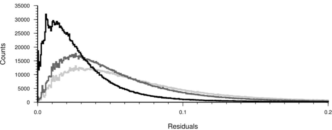
Histogram of the figure 4 shows that the enhanced peak detection method improves the estimation of the waveforms as the residuals are lower than with a unique coarse detection. Moreover the generalized Gaussian model produces the lowest residuals improving complex waveform fitting and successfully modelling flattened or peaked echoes.
Table 2 shows the results of the point extraction process. The first part of the table demonstrates that the number of waveforms for which at least one point is extracted increases by 2 to 10 % using an advanced waveform processing. The second part shows that, considering the whole contributing waveforms, advanced waveform processing increases the number of extracted points by 39 to 63%. Results are of the same order for both GA and GG models.
The position of all the extracted points is then analysed in table 3 and figure 5. Almost the whole BP point cloud is included in the AP point cloud, except for 1 % of unmatched points that were missed by the advanced processing technique. Therefore in the following lines common BP and AP points are referred to as BP points, and points detected by AP but not BP are referred to as additional points. Table 3 shows the position of the additional points compared to BP points in the wave-forms. Note that unique echoes such as ground echoes are counted in
both first and last echoes in the table. Results are in the same range for
both GA and GG models. They show that 45 to 62 % of the additional points are located below the last BP points, with last echo elevation differences ranging from -0.26 to -0.79 m depending on the plots. Most of the remaining points (27 to 47 %) are located above the first BP points, with first echo elevation differences ranging from 0.13 to 0.64 m. The maximum differences are obtained for plot 1 characterised by the highest number of additional points. Such result can be explained by the presence of multiple weak echoes in both the canopy and the low vegetation that were not detected using the basic processing technique.The high standard de-viations obtained for each plot (from 0.96 m to 2.62 m) are due to the fact that the first echo class includes common BP and AP points (e.g. first echoes such as ground echoes from unique-echo waveforms with an almost null difference between AP an BP point elevations) but also points from multiple-echo waveforms. In this latter case, the difference in elevation between the highest additional AP point above the first BP echo can reach a few meters.
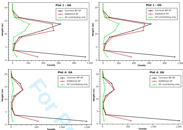
Figure 5 shows the height histograms of detected points for two plots with very different tree densitiesusing both the GA and GG models. The points were grouped into three categories: the common points between basic and advanced waveform processing point clouds called BP points (black line), all the additional points detected by the advanced processing method (which are not in the former category)(red line), and the additional points which were extracted in waveforms where no BP echo was found (green line). Note that the total number of AP points is the sum of the two first categories, the third one being part of the second category. Figure 5 shows that the newly detected points (red line) are mainly located within the canopy and in the low vegetation (up to 2.5 m). The points extracted from newly contributing waveforms (green line) have similar distribution. Globally, GA and GG models show very similar results except that the GG points inside the canopy are slightly higher than the GA points for both plots (this is especially visible for plot 1 on height histograms between 10 and 1 2 3 4 5 6 7 8 9 10 11 12 13 14 15 16 17 18 19 20 21 22 23 24 25 26 27 28 29 30 31 32 33 34 35 36 37 38 39 40 41 42 43 44 45 46 47 48 49 50 51 52 53 54 55 56 57 58 59 60
For Peer Review Only
15 m).This suggests that GG model is more sensitive to the vegetation structure.
4.2 DTM
The number of lidar points considered as terrain points is greater for all plots
when using the points extracted by the advanced processing method.
The increase is about 5 % for each plot and each model.
Surfaces computed from basic processing, Gaussian model and generalized Gaus-sian model were then compared with field measurements. Table 4 shows the mean and the standard deviation of the difference between DTMs and field measure-ments. First it is noticeable that for all plots, the difference between the two data sets is not significant (< 0.03 m) with regard to the accuracy of lidar systems (< 0.15 m on 3D points in altimetry according to lidar manufacturers): the fitted model has a weakinfluenceon the terrain point extraction.
A positive bias is observed for all plots: DTMs are higher than field measure-ments by some decimetres. More precisely, the mean and standard deviation of plot 2 are higher than they are for the other plots. It appears that field measure-ments of plot 2 are located over a narrow talweg area with irregularrelief and low vegetation which are difficult to retrieve, even after the regularization step.
In the case of regular relief area (plots 1, 3 and 4), the mean over the field measurement areas is within the accuracy of lidar systems. However, the standard deviation observed for plot 4 is twice the value of plots 1 and 3. This is attributed to the higher volume of low vegetation in this plot.
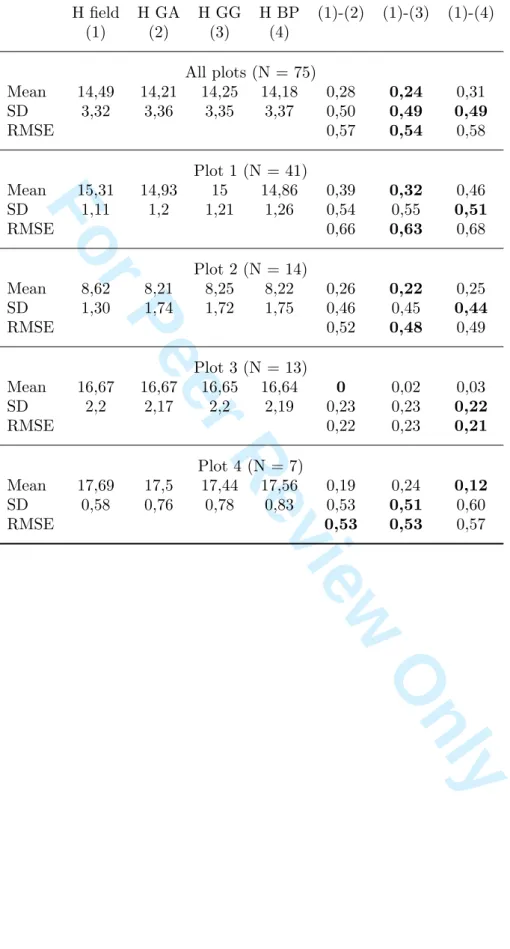
4.3 CHM-derived heights
The quality of the CHM-derived heights was evaluated on the four validation plots for a total of 75 trees (table 5, figure 6). Results show that all the three CHMs underestimate the field measured tree heights. Globally the mean underestimation is slightly reduced when using the AP data. The best results are achieved using the generalized Gaussian model, providing a mean underestimation of 0.24 m, a standard deviation of 0.49 m, and a root mean square error of 0.54 m. Compared
withthe Gaussian model and basic processing, it improves the mean value of 0.04 to 0.07 m respectively. Plot-based comparisons reveal some variability of the results depending on the stand density and ground topography. The generalized Gaussian model provides the best results for plots 1 and 2 characterised by the highest tree densities. These plots are located in different topographical configurations (table 1). At the opposite, the basic processing works better within plot 4 characterised by a very low density and a mean slope of 31.36 degrees (table 1). The best results are obtained for plot 3 characterised by a low stem density and a flat topography. For this plot, results are very similar whatever the processing method.
5. Discussion
Waveform processing combining enhanced peak detection and advanced echo mod-elling allowedthe extraction of more information comparedwithsignal process-ing currently proposed by manufacturers. The developed methods increased both the number of contributing waveforms and the total number of detected echoes within a given waveform. From the two advanced waveform processing methods tested, the one using a generalized Gaussian model had the lower residuals. This highlights that such a model is well adapted to fit complex backscattered signals
1 2 3 4 5 6 7 8 9 10 11 12 13 14 15 16 17 18 19 20 21 22 23 24 25 26 27 28 29 30 31 32 33 34 35 36 37 38 39 40 41 42 43 44 45 46 47 48 49 50 51 52 53 54 55 56 57 58 59 60
For Peer Review Only
resulting from the structure and the optical properties of vegetated areas. New waveforms contributed to the final point cloud because they contained very weak returns whose amplitude was under the detection threshold of the basic processing method. These new waveforms significantly improve the spatial sampling of dense plots and enable to better describe the crowns shape through an increased number of first echoes (figure 7).
Advanced waveform processing also increased the number of detected echoes (39 to 63 % additional echoes, table 2) due to the higher sensitivity of the peak detection method. These additional points are mainly located within the canopy and in the low vegetation. Moreover the positions of the detected first and last echoes vary compared with those obtained from basic signal processing method. The average elevation range per waveform is increased due to higher first echoes (0.13 to 0.64m in average) and a better penetration into the understorey vegetation towards the ground (-0.26 to -0.78 m in average, table 3). These quantitative values could not be directly correlated with tree height estimations, because these first and last echoes are rarely located at the top of the canopy or on the ground. Indeed most waveforms passing through the canopy are totally absorbed before reaching the ground.
The number of points classified as ground and used to compute DTMs was increased by 5 % in average using the proposed method. Field validation of the DTMs reveals very similar results whatever the method. These results are of the same order than those obtained in other studies (Hollaus et al. 2006, Reutebuch et al. 2003). A close examination of the results shows that for plots with dense low vegetation the advanced processing-based DTMs are slightly higher compared to the ones computed from the basic processing point cloud. As the advanced pro-cessing allowsthe extraction of a denser point cloud within the low vegetation, these results suggest possible classification errors that bring low vegetation points within the DTM. Such points are very difficult to separate from the ground due to the combined effects of very low height differences and steep slopes. But slope-dependent classification errors can also affect the DTM as demonstrated by Hollaus et al. (2006) over non-forested terrain using traditional multi-echo data. To address
such problems, specific classification algorithms should be developed. The
inte-gration of waveform parameters (amplitude, width and flattening) will probably improve classification using the generalized Gaussian model. Beyond these consid-erations, defining the best DTM is tricky because the differences between methods are under the precision of the georeferencing.
A lot of ecological applications use lidar-derived canopy height models to supply forest inventory (Naesset et al. 2004). By improving the number of detected echoes and the quality of the extracted points (tables 2 and 3), full-waveform lidar data is expected to provide more precise and accurate canopy height models compared with traditional multi-echo data. Our results showed lower RMSEs than the one reported in studies using multi-echo data (see Hollaus et al. (2006) for similar environmental context). Nevertheless using advanced waveform processing barely improves total tree height compared to more basic waveform processing (table 5) despite 10 to 20 % of additional contributing echoes. This is due to the fact that the newly detected echoes rarely correspond to the tree apices. Analysing the position of these points reveals that they are mainly located in the canopy or in the understory vegetation characterised by low densities that did not reflect enough energy to be detected using basic processing methods (figure 5). The main improvement of using advanced waveform processing methods to derive CHMs thus lies on the description of the crown shape and structure (figure 7). Using point-based CHM models and additional information provided by the generalized Gaussian model
1 2 3 4 5 6 7 8 9 10 11 12 13 14 15 16 17 18 19 20 21 22 23 24 25 26 27 28 29 30 31 32 33 34 35 36 37 38 39 40 41 42 43 44 45 46 47 48 49 50 51 52 53 54 55 56 57 58 59 60
For Peer Review Only
(alpha parameterwill probably bring further improvements.
6. Conclusion
Enhanced peak detection algorithm combined with an advanced echo modelling including Gaussian and generalized Gaussian models significantly increases the number of detected echoes. Point-based and grid-based analyses showed that the additional points mainly describe the internal crown structure and the low vegeta-tion stratum. Therefore, while DTM and CHM-based heights are not significantly improved, the additionally extracted points could be efficiently used to characterise the detailed vegetation structure such as crown properties and tree regeneration under the canopy. If the peak detection method is not crucial to compute DTMs, because they are still limited by errors due to georeferencing, classification, and interpolation, it showed to be of great interest to better sample tree crowns and improve RMSEs on height measurements. Moreover the integration of echo shape parameters of thegeneralized Gaussian model will provide information on both shape and optical properties of the targets. Hence valuable information will be available for driving ground point classification and characterising vegetation type and structure. But as long as only geometric information is used, advanced pro-cessing based on Gaussian model is a good compromise. Despite a better fitting performance, the generalized Gaussian model is slower to compute and generates noise within the point cloud due to fitting complexity.
Compared with current fitting techniques, the proposed advanced echo detection method allowed to greatly improve the number of de-tected echoes within forest canopies. Because a large number of the additional detected echoes lies within the lower canopy and in the under-storey, the description of the vegetation vertical structure is expected to be improved. Such information is crucial to quantify the 3D organisation of forest covers and to derive information about the forest succession and the status of regeneration. Compared with traditional multi-echo derived parameters, advanced processing of full-waveform data will al-low to extract additional indicators of the vegetation structural charac-teristics correlated to high level forest products (e.g. volume, biomass, canopy fuel or carbon content), opening up the possibility to develop prediction models of forest parameter performing over a large range of environmental conditions.
-Acknowledgements
The authors would like to thank Laurent Albrech for his valuable help in field data collection and post-processing. This work is part of the ExFOLIO project and was realized thanks to the financial support of the CNES (Centre National d’ ´Etudes Spatiales). The authors would also like to deeply thank the GIS Draix for providing the full-waveform lidar data and for helping in ground truth surveys. They are grateful to INSU for its support to GIS Draix through the ORE program.
1 2 3 4 5 6 7 8 9 10 11 12 13 14 15 16 17 18 19 20 21 22 23 24 25 26 27 28 29 30 31 32 33 34 35 36 37 38 39 40 41 42 43 44 45 46 47 48 49 50 51 52 53 54 55 56 57 58 59 60
For Peer Review Only
References
Ahokas, E., Kaartinen, H. and Hyypp¨a, J., 2003, A Quality Assessment of Airborne Laser Scanner Data. In Proceedings of the International Archives of Photogrammetry, Remote Sensing and Spatial Information Sciences, 34 (Part 3/W13), Oct., Dresden, Germany, pp. 1–7.
Andersen, H.E., Reutebuch, S. and Schreuder, G., 2001, Automated indi-vidual tree measurement through morphological analysis of a LIDAR-based canopy surface model. In Proceedings of the Proceedings of First International Precision Forestry Symposium (Seattle,18-19 June 2001), pp. 11–22.
Anderson, J., Martin, M., Dubayah, M.L.S.R., Hofton, M., Hyde, P., Peterson, B., Blair, J. and Knox, R., 2006, The use of waveform lidar to measure northern temperate mixed conifer and deciduous forest structure in New Hampshire. Remote Sensing of Environment, 105, pp. 248–261. Axelsson, P., 1999, Processing of laser scanner data - algorithms and
applica-tions. ISPRS Journal of Photogrammetry & Remote Sensing, 54, pp. 138–147. Blair, J., Rabine, D. and Hofton, M., 1999, The Laser Vegetation Imaging Sensor: a medium-altitude digitisation-only, airborne laser altimeter for map-ping vegetation and topography. ISPRS Journal of Photogrammetry & Remote Sensing, 54, pp. 115–122.
Bretar, F. and Chehata, N., 2008, Terrain Modelling from lidar range data in natural landscapes: a predictive and Bayesian framework. Tech-nical report, Institut G´eographique National. Available at http://hal. archives-ouvertes.fr/hal-00278942/fr/.
Chauve, A., Mallet, C., Bretar, F., Durrieu, S., Pierrot-Deseilligny, M. and Puech, W., 2007, Processing full-waveform lidar data: modelling raw signals. In Proceedings of the International Archives of Photogrammetry, Remote Sensing and Spatial Information Sciences, 36 (Part 3/W52), Sep., Espoo, Finland, pp. 102–107.
Dubayah, R., Knox, R., Hofton, M., Blair, J. and Drake, J., 2000, Land surface characterization using lidar remote sensing. In Proceedings of the Spa-tial Information for Land Use Management, Sydney, Australia, pp. 25–38. Gaveau, D. and Hill, R., 2003, Quantifying canopy height underestimation by
laser pulse penetration in small-footprint airborne laser scanning data. Cana-dian Journal of Remote Sensing, 29, pp. 650–657.
Hodgson, M.E. and Bresnahan, P., 2004, Accuracy of airborne lidar-derived el-evation: empirical assessment and error budget. Photogrammetric Engineering & Remote Sensing, 70, pp. 331–339.
Hofton, M., Minster, J. and Blair, J., 2000, Decomposition of Laser Altimeter Waveforms. IEEE Transactions on Geoscience and Remote Sensing, 38, pp. 1989–1996.
Hollaus, M., Wagner, W., Eberhofer, C. and Karel, W., 2006, Accuracy of large-scale canopy heights derived from LiDAR data under operational con-straints in a complex alpine environment. ISPRS Journal of Photogrammetry and Remote Sensing, 60, pp. 323–338.
Hopkinson, C., Chasmer, L., Lim, K., Treitz, P. and Creed, I., 2006, To-wards a universal lidar canopy height indicator. Canadian Journal of Remote Sensing, 32, pp. 139–152.
Hyyppa, J., Kelle, O., Lehikoinen, M. and Inkinen, M., 2001, A segmentation-based method to retrieve stem volume estimates from 3-D tree hight models produced by laser scanners. IEEE Transactions Geosciences and Remote Sensing, 39, pp. 969–975. 1 2 3 4 5 6 7 8 9 10 11 12 13 14 15 16 17 18 19 20 21 22 23 24 25 26 27 28 29 30 31 32 33 34 35 36 37 38 39 40 41 42 43 44 45 46 47 48 49 50 51 52 53 54 55 56 57 58 59 60
For Peer Review Only
Jutzi, B. and Stilla, U., 2005, Waveform processing of laser pulses for re-construction of surfaces in urban areas. In Proceedings of the International Archives of Photogrammetry, Remote Sensing and Spatial Information Sci-ences, 36 (Part 8/W27), Mar., Tempe, USA.
Kobler, A., Pfeifer, N., Ogrinc, P., Todorovski, L., Ostir, K. and Dze-roski, S., 2007, Repetitive interpolation: A robust algorithm for DTM gener-ation from Aerial Laser Scanner Data in forested terrain. Remote Sensing of Environment, 108, pp. 9–23.
Lefsky, M., Cohen, W., Acker, S., Parker, G., Spies, T. and Harding, D., 1999, Use of large-footprint scanning airborne LiDAR to estimate forest stand characteristics in the Western Cascade of Oregon. Remote Sensing of Environment, 67, pp. 2.
Lim, K., Treitz, P., Wulder, M., Saint-Onge, B. and Flood, M., 2003, LiDAR remote sensing of forest structure. Progress in Physical Geography, 27, pp. 88–106.
Lloyd, C.D. and Atkinson, P.M., 2002, Deriving DSMs from LiDAR data with kriging. International Journal of Remote Sensing, 23, pp. 2519–2524.
Magnussen, S. and Boudewyn, P., 1998, Derivations of stand heights from airborne laser scanner data with canopy-based quantile estimators. Canadian Journal of Remote Sensing, 28, pp. 1016–1031.
Naesset, E., 1997, Determination of mean tree height of forest stands using air-borne laser scanner data. ISPRS Journal of Photogrammetry & Remote Sens-ing, 52, pp. 49–56.
Naesset, E., Gobakken, T., Holmgren, J., Hyyppa, H., Hyyppa, J., Mal-tamo, M., Nilsson, M., Olsson, H., Persson, A. and Soderman, U., 2004, Laser scanning of forest resources: The Nordic experience. Scandinavian Journal of Forest Research, 19, pp. 482–499.
Persson, A., Holmgren, J. and S¨oderman, U., 2002, Detecting and measuring individual trees using an airborne laser scanner. Photogrammetric Engineering and Remote Sensing, 68, pp. 925–932.
Persson, A., S¨oderman, U., T¨opel, J. and Alhberg, S., 2005, Visualization and Analysis of Full-Waveform Airborne Laser Scanner Data. In Proceedings of the International Archives of Photogrammetry, Remote Sensing and Spatial Information Sciences, 36 (Part 3/W19), Sep., Enschede, The Netherlands, pp. 103–108.
Reitberger, J., Krzystek, P. and Stilla, U., 2006, Analysis of Full-Waveform Lidar Data for Tree Species Classification. In Proceedings of the International Archives of Photogrammetry, Remote Sensing and Spatial Information Sci-ences, 36 (Part 3), Sep., Bonn, Germany, pp. 228–233.
Reutebuch, S., McGaughey, R., Andersen, H.E. and Carson, W., 2003, Accuracy of a high-resolution lidar terrain model under a conifer forest canopy. Canadian Journal of Remote Sensing, 29, pp. 527–535.
Sithole, G. and Vosselman, G., 2004, Experimental comparison of filter algo-rithms for bare-Earth extraction from airborne laser scanning point clouds. ISPRS Journal of Photogrammetry and Remote Sensing, 59, pp. 85–101. Steinvall, O., 2000, Effects of Target Shape and Reflection on Laser Radar Cross
Sections. Applied Optics, 39, pp. 4381–4391.
Vepakomma, U., St-Onge, B. and Kneeshaw, D., 2008, Spatially explicit char-acterization of boreal forest gap dynamics using multi-temporal lidar data. Remote Sensing of Environment, 112, pp. 2326–2340.
Wagner, W., Ullrich, A., Ducic, V., Melzer, T. and Studnicka, N., 2006, Gaussian Decomposition and calibration of a novel small-footprint
full-1 2 3 4 5 6 7 8 9 10 11 12 13 14 15 16 17 18 19 20 21 22 23 24 25 26 27 28 29 30 31 32 33 34 35 36 37 38 39 40 41 42 43 44 45 46 47 48 49 50 51 52 53 54 55 56 57 58 59 60
For Peer Review Only
waveform digitising airborne laser scanner. ISPRS Journal of Photogrammetry & Remote Sensing, 66, pp. 100–112.
Wagner, W., Ullrich, A., Melzer, T., Briese, C. and Kraus, K., 2004, From single-pulse to full-waveform airborne laser scanners: Potential and prac-tical challenges. International Archives of Photogrammetry, Remote Sensing and Spatial Information Sciences, 35 (Part B3), pp. 201–206.
1 2 3 4 5 6 7 8 9 10 11 12 13 14 15 16 17 18 19 20 21 22 23 24 25 26 27 28 29 30 31 32 33 34 35 36 37 38 39 40 41 42 43 44 45 46 47 48 49 50 51 52 53 54 55 56 57 58 59 60
For Peer Review Only
Table 1. Characteristics of the validation plots.
Topography Vegetation
Plot
Plot Elevation Slope
Aspect
Mean Height DBH
radius mean±SD mean±SD density mean±SD mean±SD
(m) (m) (%) (stem/ha) (m) (m) 1 15 1163.21 (4.35) 15.35 (7.75) southest 771 14.1(2.7) 0.21 (0.05) 2 15 857.69 (8.20) 33.57 (21.36) southwest 300 7.3(2.54) 0.13 (0.06) 3 15 853.85 (1.43) 6.17 (3.25) south 242 15.1(3.95) 0.28 (0.08) 4 15 862.75 (6.81) 31.36 (18.99) southwest 100 17.7(0.58) 0.27 (0.01) 1 2 3 4 5 6 7 8 9 10 11 12 13 14 15 16 17 18 19 20 21 22 23 24 25 26 27 28 29 30 31 32 33 34 35 36 37 38 39 40 41 42 43 44 45 46 47 48 49 50 51 52 53 54 55 56 57 58 59 60
For Peer Review Only
Table 2. Overall statistics on waveforms and point extraction.
Plots 1 2 3 4
Number of contributing waveforms
BP 2447 2809 3274 2859 GA 2673 2865 3351 2921 GG 2672 2865 3353 2921 Point extraction Nb BP points 2792 3338 3886 3240 Nb GA points 4496 4669 5471 4496 % additional points 61 40 41 39 Nb GG points 4563 4708 5531 4546 % additional points 63 41 42 40 1 2 3 4 5 6 7 8 9 10 11 12 13 14 15 16 17 18 19 20 21 22 23 24 25 26 27 28 29 30 31 32 33 34 35 36 37 38 39 40 41 42 43 44 45 46 47 48 49 50 51 52 53 54 55 56 57 58 59 60
For Peer Review Only
Table 3. Statistics on additional AP extracted points compared to BP points.
Plots 1 2 3 4
Position of additional points compared to BP points: GA/GG
% above first BP 33/33 31/27 32/28 47/45
% between first and last 5/5 11/11 16/15 8/8
% below last BP 62/61 58/61 52/57 45/47
First and last echoes elevation differences (AP - BP) (m): GA/GG
1st echo (mean) 0.64/0.63 0.14/0.13 0.42/0.41 0.32/0.30 1st echo (SD) 2.62/2.62 0.97/0.96 2.10/2.10 1.53/1.51 last echo (mean) -0.78/-0.79 -0.38/-0.40 -0.44/-0.50 -0.26/-0.23 last echo (SD) 2.58/2.59 1.53/1.51 1.89/2.01 1.71/1.72 1 2 3 4 5 6 7 8 9 10 11 12 13 14 15 16 17 18 19 20 21 22 23 24 25 26 27 28 29 30 31 32 33 34 35 36 37 38 39 40 41 42 43 44 45 46 47 48 49 50 51 52 53 54 55 56 57 58 59 60
For Peer Review Only
Table 4. Field validation of the derived DTMs (50 cm resolution). Results are the signed differences of elevation between DTM cell values and field points.
Plots 1 2 3 4 Nb field points 69 84 65 64 BP mean±SD (m) 0.08±0.09 0.37±0.34 0.13±0.18 0.14±0.28 GA mean±SD (m) 0.09±0.10 0.33±0.29 0.11±0.17 0.19±0.32 GG mean±SD (m) 0.10 ±0.10 0.38±0.36 0.12±0.17 0.17±0.29 1 2 3 4 5 6 7 8 9 10 11 12 13 14 15 16 17 18 19 20 21 22 23 24 25 26 27 28 29 30 31 32 33 34 35 36 37 38 39 40 41 42 43 44 45 46 47 48 49 50 51 52 53 54 55 56 57 58 59 60
For Peer Review Only
Table 5. Statistics of the field versus CHM-based total tree height measurements. Field values are compared to values extracted from Gaussian model (GA), generalized Gaussian model (GG), and basic processing (BP).
H field H GA H GG H BP (1)-(2) (1)-(3) (1)-(4) (1) (2) (3) (4) All plots (N = 75) Mean 14,49 14,21 14,25 14,18 0,28 0,24 0,31 SD 3,32 3,36 3,35 3,37 0,50 0,49 0,49 RMSE 0,57 0,54 0,58 Plot 1 (N = 41) Mean 15,31 14,93 15 14,86 0,39 0,32 0,46 SD 1,11 1,2 1,21 1,26 0,54 0,55 0,51 RMSE 0,66 0,63 0,68 Plot 2 (N = 14) Mean 8,62 8,21 8,25 8,22 0,26 0,22 0,25 SD 1,30 1,74 1,72 1,75 0,46 0,45 0,44 RMSE 0,52 0,48 0,49 Plot 3 (N = 13) Mean 16,67 16,67 16,65 16,64 0 0,02 0,03 SD 2,2 2,17 2,2 2,19 0,23 0,23 0,22 RMSE 0,22 0,23 0,21 Plot 4 (N = 7) Mean 17,69 17,5 17,44 17,56 0,19 0,24 0,12 SD 0,58 0,76 0,78 0,83 0,53 0,51 0,60 RMSE 0,53 0,53 0,57 1 2 3 4 5 6 7 8 9 10 11 12 13 14 15 16 17 18 19 20 21 22 23 24 25 26 27 28 29 30 31 32 33 34 35 36 37 38 39 40 41 42 43 44 45 46 47 48 49 50 51 52 53 54 55 56 57 58 59 60
For Peer Review Only
Figure 1. Principle of lidar acquisition and processings.
1 2 3 4 5 6 7 8 9 10 11 12 13 14 15 16 17 18 19 20 21 22 23 24 25 26 27 28 29 30 31 32 33 34 35 36 37 38 39 40 41 42 43 44 45 46 47 48 49 50 51 52 53 54 55 56 57 58 59 60
For Peer Review Only
Figure 2. 3D view of the study site.
1 2 3 4 5 6 7 8 9 10 11 12 13 14 15 16 17 18 19 20 21 22 23 24 25 26 27 28 29 30 31 32 33 34 35 36 37 38 39 40 41 42 43 44 45 46 47 48 49 50 51 52 53 54 55 56 57 58 59 60
For Peer Review Only
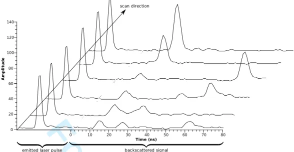
A m p li tu d e 0 20 40 60 80 100 120 140 0 10 20 30 40 50 60 70 80 Time (ns) scan directionemitted laser pulse backscattered signal
Figure 3. Examples of lidar waveforms showing the recorded backscattered signals for a set of successive laser pulses. 1 2 3 4 5 6 7 8 9 10 11 12 13 14 15 16 17 18 19 20 21 22 23 24 25 26 27 28 29 30 31 32 33 34 35 36 37 38 39 40 41 42 43 44 45 46 47 48 49 50 51 52 53 54 55 56 57 58 59 60
For Peer Review Only
0 5000 10000 15000 20000 25000 30000 35000 C ou nt s 0.0 0.1 0.2 ResidualsFigure 4. Histograms of fitting residuals: Gaussian model and coarse detection in grey, Gaussian model and enhanced detection in dark grey, generalized Gaussian model and enhanced detection in black.
1 2 3 4 5 6 7 8 9 10 11 12 13 14 15 16 17 18 19 20 21 22 23 24 25 26 27 28 29 30 31 32 33 34 35 36 37 38 39 40 41 42 43 44 45 46 47 48 49 50 51 52 53 54 55 56 57 58 59 60
For Peer Review Only
H e ig h t (m ) 0 5 10 15 20 Counts 0 200 400 600 800 1,000 Common BP AP Additional AP AP contributing only Plot 1 : GA H e ig h t (m ) 0 5 10 15 20 Counts 0 200 400 600 800 1,000 Common BP AP Additional AP AP contributing only Plot 1 : GG H e ig h t (m ) 0 5 10 15 20 Counts 0 500 1,000 1,500 Common BP AP Additional AP AP contributing only Plot 4: GA H e ig h t (m ) 0 5 10 15 20 Counts 0 500 1,000 1,500 Common BP AP Additional AP AP contributing only Plot 4: GGFigure 5. Height histograms for plots 1 and 4. Common points computed from basic processing (BP) and advanced processing (AP) (black line), additional AP points (red line), and points extracted from waveforms only contributing to AP (green line).
1 2 3 4 5 6 7 8 9 10 11 12 13 14 15 16 17 18 19 20 21 22 23 24 25 26 27 28 29 30 31 32 33 34 35 36 37 38 39 40 41 42 43 44 45 46 47 48 49 50 51 52 53 54 55 56 57 58 59 60
For Peer Review Only
● ● ● ● ●● ● ● ● ● ● ● ● 5 10 15 20 5 10 15 20 Field height (m) Lidar height (m) ● Plot 1 Plot 2 Plot 3 Plot 4 (a) BP ● ● ● ● ● ● ● ● ● ● ● ● ● 5 10 15 20 5 10 15 20 Field height (m) Lidar height (m) ● Plot 1 Plot 2 Plot 3 Plot 4 (b) GA ● ● ● ● ●● ● ● ● ● ● ● ● 5 10 15 20 5 10 15 20 Field height (m) Lidar height (m) ● Plot 1 Plot 2 Plot 3 Plot 4 (c) GG 1 2 3 4 5 6 7 8 9 10 11 12 13 14 15 16 17 18 19 20 21 22 23 24 25 26 27 28 29 30 31 32 33 34 35 36 37 38 39 40 41 42 43 44 45 46 47 48 49 50 51 52 53 54 55 56 57 58 59 60For Peer Review Only
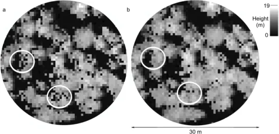
Figure 7. Difference in crown representation between basic processing (a) and advanced processing-based CHM (b). Advanced processing gives rise to an increase in first echo spatial density resulting to an improved crown description with the removal of some gaps. Circles highlight major improvements.
1 2 3 4 5 6 7 8 9 10 11 12 13 14 15 16 17 18 19 20 21 22 23 24 25 26 27 28 29 30 31 32 33 34 35 36 37 38 39 40 41 42 43 44 45 46 47 48 49 50 51 52 53 54 55 56 57 58 59 60