Adaptive swing-up and balancing control of acrobot systems

Adaptive Swing-up and Balancing Control of Acrobot Systems

by

Luke B. Johnson

Submitted to the Department of Mechanical Engineering in Partial Fulfillment of the Requirements for the

Degree of Bachelor of Science at the Massachusetts Institute of Technology

June 2009

@ 2009 Massachusetts Institute of Technology All rights reserved

MASSACHUSETTS INSTITUTE OFTECHNOLOGY

SEP 1 6 2009

LIBRARIES

ARCHIVES

Department of Mechanical Engineering May 11, 2009

/4 /3/

Certified by .... ...

John J. Leonard Professor of Mechanical Engineering

- esis Supervisor

Accepted by ... ...

Professor J. Lienhard V Collins Professor of Mechanical Engineering

Adaptive Swing-up and Balancing Control of Acrobot Systems

by

Luke B. Johnson

Submitted to the Department of Mechanical Engineering on May 11, 2009 in Partial Fulfillment of the Requirements for the Degree of Bachelors of Science in

Mechanical Engineering

Abstract

The field of underactuated robotics has become the core of agile mobile robotics research. Significant past effort has been put into understanding the swing-up control of the

acrobot system. This thesis implements an online, adaptive swing-up and balancing controller with no previous knowledge of the system's mass or geometric parameters. A least squares method is used to identify the 5 parameters necessary to completely

characterize acrobot dynamics. Swing up is accomplished using partial feedback linearization and a pump up strategy to add energy to the system. The controller then catches the swung up system in the basin of attraction of an LQR controller computed using the estimated parameter values generated from online system identification. These results are then simulated using a MATLAB simulation environment.

Thesis Supervisor: John J. Leonard

Introduction

Adaptive algorithms have been extensively successful in industrial applications where arm mass parameters undoubtedly change when interacting with their

environments. This interaction forces control algorithms to adapt to these changes and continuously update their estimated model of the system. The basic idea behind all types

of adaptive control is to create a skeleton model with some unknown parameters am that

combine with some measureable quantities f, and y to form constraint equations. A linear version of this constraint is shown below as Equation 1

y = a, f (q) + a2f,(q) + ...+ am fm (q)" ()

Any number of update laws can be used to estimate the unknown parameters am, and

given sufficiently diverse set of fm 's we can obtain an arbitrarily precise estimate of the system's true dynamics.

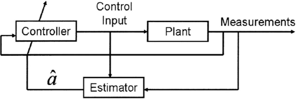
There are a couple different "flavors" of adaptive control algorithms. This paper specifically uses the model known as a self tuning controller. A block diagram of this model is shown in Figure 1 below.

Control

Input

Measurements

Controller

Plant

Estimat

_or

Figure 1: Block diagram of a self tuning controller, where i is defined as a vector of the current best estimate of the system parameters

In the figure above the "controller" is the law that defines the control input, the "plant" is the unchangeable system dynamics, the output of the plant is what is measurable, the control input is the output of the controller, and both the measurements and the control

input are passed into an "estimator" that produces a vector of the current best guess of the parameters, a.

The industrial implementation of adaptive control is slightly different because control engineers are often interested in following specified trajectories for arms with unknown parameters. This gives rise to a particularly elegant form of adaptive control call Model-Reference Adaptive Control [1]. This implementation uses linear feedback around the desired trajectory and generally leads to very fast convergence and excellent performance. Unfortunately this method is not quite adequate to handle underactuated robotics as it is defined. By the definition of underactuated systems, certain desired accelerations are simply unattainable (in the acrobot case this is because there is no actuator on one of the joints.) The controller in underactuated cases is more usually concerned with reaching goals. The case study presented in this paper is specifically attempting to swing up the acrobot and balance in the unstable vertical position. The problem with doing simple trajectory planning is that we may not know ahead of time what type of trajectories are possible, given the actuator limits. Thus we are left using the slightly less profound self tuning model of adaptive control.

Why the acrobot?

Up until this point I have been generic about talking about "underactuated

systems." This thesis focuses on the case study of an acrobot system. The reasons behind choosing this system are not completely arbitrary. 1) The acrobot has been extensively studied and therefore there is extensive previous literature on the problem. 2) Part of the convenient nature of the acrobot system is that it has a constrained state space on position. An unstable acrobot system when system id is poor will not drive itself around the room while learning to swing up like a cart-pole system might have to. 3) The acrobot system is easy to reset after a failed attempt, a controller of virtual damping between links 1 and 2 will bring the system back to its stable equilibrium.

As was mentioned above, the swing up control of the acrobot has been

extensively explored. In [2], Spong outlines a swing up controller using already known mass parameters. The method presented in Spong's paper for swing up is what this paper uses as a base for its swing up controller. As will be explained later in the paper, this

choice was most likely not ideal for the purposes of this problem. The method as Spong proposed it assumed a strict system identification before the controller will run. In [3] calibration is addressed using an Unscented Kalman filter to obtain system parameters, but it too is run offline ahead of time, in order to guarantee strict error tolerances on the system parameters before the swing up attempt was run. One note about this paper is they use a relatively new Lyaponov based scheduling procedure for the balancing controller that may have solved some of the swing up to LQR switching instability that was incurred under this paper's implementation.

Experimental Setup

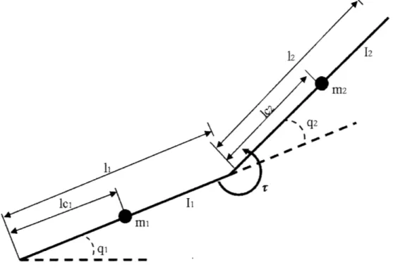
The entire system was simulated in a MATLAB environment. Figure 2 below outlines the geometry of the acrobot arm as well as the relevant system parameters.

1, \ q2 -0

4-I

mi

Figure 2: geometry of the acrobot arm as well as the relevant system parameters

As seen in the figure above, qi is the angle of the ith link, mi is the mass of the ith link,

1i is the length of the ith link, 1,i is the length from the base joint of link i to the center of

mass of length i, 1i is the moment of inertia of the ith link about the center of mass, and

r is the input torque applied. The equations of motion of the system are listed below as Equations 2 and 3 and are also verified in [2]:

dl lql + dl1q2 + h1 + 0 = 0, (2)

d1 241 + d2q2 + h2 + 2 = 'r (3)

In these equations ij, is the second derivative of the ith angular measurement. The other constants used in Equations 2 and 3 are defined in Equations 4-10

dl, = m,1( + m2 (1 + 1,2 2 + 21,1,2 cos(q2 ))+ I 12 (4) d22 = 21 22 + 1" (5) dl2 = 2 ( 2 + 11 c2 cos(q2)) + _{I1 (6)} h, = -m1 1l,.2 sin( q )c) - 2m2 1l. 2 sin( q2 )q2q1 (7) h2 = m211,.2 sin(q2

)A'

where g is the acceleration due to gravity, and ), is the first derivative of the angular position of the ith link.

The system is modeled as a continuous time system integrated with MATLAB's ode45 implementation of Runga Kutta 4. The input torque is modeled as a continuous input that is held constant during each sampling interval to help simulate how a physical system would be controlled. The values for the simulation constants are shown below in Table 1.

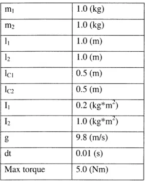
Table 1: values of simulation constants with their associated units mi 1.0 (kg) m2 1.0 (kg) 11 1.0 (m) 12 1.0 (m) Ici 0.5 (m) IC2 0.5 (m) I1 0.2 (kg*m2) 12 1.0 (kg*m2) g 9.8 (m/s) dt 0.01 (s) Max torque 5.0 (Nm)

In this simulation, q , 1 , q2 2 are assumed to be measureable and are treated as a the

complete set of state variables. If these quantities were not measurable we would have to create an estimator. If this were the case it might be easiest to use an Unscented Kalman Filter such as in [3], to perform both the state estimation and parameter estimation. For the purposes of this paper this was assumed to be too complicated and thus the fully

observable assumption was maintained.

Swing up implementation

The design purpose of the swing up controller is to move the acrobot system into a state contained within the basin of attraction of the LQR controller for successful balancing. In order to decrease the complexity of the swing up controller we use partial feedback linearization (PFL) on link 2 in or order to decouple the influence of link 1 on link 2's dynamics. This derivation is shown in [2] but an abridged version is shown here for completeness. If we rearrange Equation 2 we obtain Equation 11 shown as

Equation 11 can then be substituted into Equation 3 to produce Equation 12,

dzzq2 + h, + 02 = , (12)

where d22, h, 02 are defined in Equations 12-15 as

d 2 =d 22 - d21 - d-'d1 , (13)

h2 = h2 - d1d d'h, (14)

02 = 2 - d2 1d 1 . (15)

This is a convenient form for implementing PFL because with the assumption that we have sufficiently large torque allowances, we can define the input r in Equation 12 as Equation 16,

S= d,,v, + h, + , (16)

where v2 is the desired link 2 angular acceleration. This completely decouples the actions of link 1 with link 2. (Note the actions of link 2 still influence link 1 but not vice-versa) This result in illustrated in the Equations 17 and 18 below as

d,1lq + h, + 01 = -d1 2v2, (17)

2 v2". (18)

It is notable that although the motions on link 1 do not affect link 2 with this control strategy (all the inertial coupling is canceled out through the PFL), the control input v2 does and must affect the motion of link 1. It is this inertial coupling that we use

to swing up the acrobot, all the while maintaining complete control authority of12 . After this PFL we must decide what control input we do want to implement such that q, swings

up, while keeping q2 under control. [2] proposes the following desired trajectory of link

2, as shown in Equation 19

2a

q = _{- tan (c), (19)}

What this desired trajectory effectively does is smoothly keep q2 between the angles of

+a . More importantly, the net torque required to follow this desired input forces energy into the system (this is only necessarily true if there is sufficient torque to hold the PFL constraints.) This way of pumping energy into the system turns out to be both convenient

and troublesome as will be described later in the paper. The controller to obtain this desired trajectory is then a PD controller as shown in Equation 20,

v2 = k,, (q" - q2) - kd,2 , (20)

where k, is the proportional gain and kd is the derivative gain. If the arm parameters where known a priori, a method such as stochastic gradient descent could be used to tune these gains for optimal performance. Since the controller needs to adapt to a wide range of arm parameters, they are kept constant. The parameters used in this simulation are shown in table 2 below

Table 2: swing up simulation parameters

k, 400

kd 10

U 0.75

Adaptation techniques

As has been mentioned above there are many ways to perform online system identification. The method that was used in this implementation is least squares estimation. The final implementation combines a batch least squares method when the

input is non-rich, with a recursive update that takes over when the input is sufficiently rich to effectively update every time step. The initial batch data was necessary to give legitimate initial conditions to the recursive least squares (RLS) algorithm. For non-rich data, the RLS algorithm was converging to significantly wrong local minima when random initial conditions were given. In order to frame the dynamic equations to be compatible with least squares estimation, the state equations were parameterized using 5 variables as shown below in Equations 21-25 as:

a1 = m212 +mzl + mlc + 1I + 12 (21)

a2 = mzll1, 2 (22)

a3 = m2 22 (23)

a4 = (m1l,1. + mzl )g (24)

a5 = m21,2g (25)

These 5 parameters are then plugged into Equations 2 and 3 and using the shorthand defined in Equations 26-29 below

c12 = cos(q, + q2), (26)

C1 = cos(ql), (27)

c2 = cos(q2), (28)

s2 = sin(q2), (29)

the dynamic equations of the acrobot system become Equations 30 and 31,

alj1 + a2 (2c,2q + C2 2 -S - 2S2q42 + a3 2 a4c + a5c12 = 0, (30)

a, (0) + a2 (c2i1 + S2l) + a3(q 9 +

4

These equations are not especially convenient to perform least squares on separately because equation 31 especially gives rise to a notably insufficiently rich set of inputs

values to the least squares algorithm. In an attempt to resolve this, Equations 30 and 31 above are combined to create Equation 32,

a,

q

q2+

a3(2q, + , )+a 4c1+2ac 12=r

(32)

a significantly more diverse input equation which also maintains the final linear form that will be used in the least squares parameter estimation of a...a5. Equation 33 below

aiu1 + a2u, +... + amm = y (33)

is the basic linear form required for least squares estimation. Our simulation environment assumes q ,q1,q,,q2 are all known, so if we estimate q,1,q2 as Equation 34 below

i (t)- 4 (t -1)(34)

Then we have all of the information to needed to compute the lease squares inputs u ...u5.

The formula for least squares estimation then requires that we define a vector of parameters as Equation 35 below

a = [al...am T _{, (35)}

as well as a vector of inputs, shown as Equation 36

(36)

then we can rewrite Equation 33 in its companion vector form as Equation 37,

From this form we can refer to the formula for Least Squares approximation batch processing from [4] and this becomes Equation 38 below

a = PB (38)

where P is defined below as Equation 39

P = ((p(t)' (t)), (39)

t=1

and B is defined as Equation 40

N

B = , y(t)p(t).. (40)

t=1

This batch algorithm is very good a building up a P- matrix with sparse data (as it occurs when the system is either near its relaxed vertical or is stabilizing at the top.) During early swing up the parameters remain at their initial conditions as defined (all l's). The algorithm decides when the determinant of the P matrix is greater than 1 to seed the RLS algorithm with this batch computation.

The RLS algorithm creates a refined parameter estimate every time step. The parameter update equation is shown below as Equation 40 is derived in [4]

a(t) = i(t -1)+ ( (p (t)p y(t)- (t)(t-1)) (40)

This update also requires an update in P matrix as shown below as Equation 41 which is also derived in [4]

P,_ ((t)(pT (t)p_l

P, = P,_ ₍₄₁₎

The initial parameter estimates are the result of the batch estimate shown in Equation 42,

^(O) = PB (42)

The initial condition for P is just a 5x5 identity matrix.

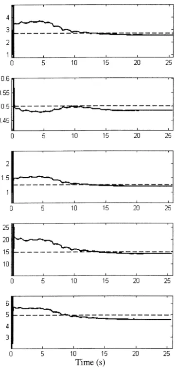
Figure 3 below shows plots of estimated parameters (solid line) versus the true value of the parameters (dotted line) with respect to time. As we can see from Figure 3, the first fraction of a second is very chaotic with respect to the parameter estimates. This corresponds to when the acrobot has just started moving and the least squares algorithm has yet to measure a diverse enough set of inputs to warrant a precise measurement. In well under a second we can see the estimated value of the parameters jump to somewhat consistent values and slowly begin to converge to near their true values. Each of the parameters converges to their true value within 5%. This is more than enough accuracy to accurately perform PFL, and as we will see in Figure 4, this is good enough to suggest complete convergence of the LQR controller.

4 3 ----2 0 5 10 15 20 25 0.6 0.55 0.5 0.5 --- --- --0.45 0 5 10 15 20 25 2 1.5 1 0 5 10 15 20 25 25 20 15 10 0 5 10 15 20 25 0 5 10 15 20 25 Time (s)

Figure 3: Plots of estimated parameter values versus true value of the parameter values with respect to time. The dotted line represents the true parameter values and the solid line represents the time history of the estimated parameter values.

A note about this method is that it will not handle time varying parameters well, but an adaptation of the Recursive least squares method using a decaying exponential of

previous estimate can be used. The equations for this process are shown below as Equations 43 and 44 and are documented in [4],

0,(t) = O(t - 1) + ( (,T ( (t) y(t)-'(t)(t 1 (43)

1 P + (t) (t)P1

P (a +p ( (t)p t

(44)

This exponential weighting method is not implemented but could be substituted if the arm parameters are expected to vary in time continuously or in an undetectable way such that we would need to autonomously pick up the change. It is worth note that this method is slightly complicated by the nature that P decreases exponentially fast depending on the value of 8. This requires a Pt resetting every 20 or so steps, so complications may arise with resetting P matrices during a series of insufficiently rich

data collections. For these reasons this addition is not implemented in the final model.

LQR stabilization

The above swing up methods will only get the acrobot near its upright balancing position. When the acrobot is close to stabilizing near the top an LQR method is used to converge the system to balancing upright in the configuration q, = --. , q, ₂ = 0, q2 = 0,

and )2 = 0. In order to create this LQR controller, the non-linear dynamics need to be linearized around the upright position. To do this, we first change variables defining q, * in Equation 45 below as

q* = q, (45)

2

The non-linear terms there then linearized. This means that all of the second order terms are considered zero and the trigonometric functions are then converted via Equations 46 and 47 shown below

cos(q,) = -q, *

cos(q, + q2) = -[q2+ ql*]

(46) (47)

When the original non-linear equations (Equations 30 and 31) are linearized, we obtain the following differential equations shown as Equations 48 and 49

(a3a4 -a 2a5)q *-a 2a5q2 - (a3+ a2)zr

2 2

a1a3- 3 a2

(aia5 + a2a5 -a 3a4 -a 2a4 -a 3a5)q * +(ala5 + a2a5 -a 3a5)q 2 (al + 2a2 )r

q2 2 2

a1a3 - a3 - a2

We can then define our state space as shown in Equation 50 as

q = (qj*,4 ,,q2, q2)

(48)

(49)

(50)

Then transforming the above differential equations into a state space representation we get an equation shown below, Equation 51

(51)

Where the A matrix is defined in Equation 52,

0 (a₂a₃ -a ₂a₅) 2 2 ala3 - a_{3 2} (aa , 5 + a2a5 - a3a4 -a 2a 4 -a 3a5) aa 3 -2

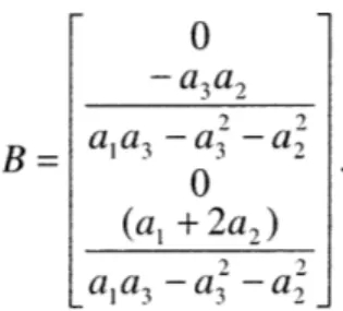
and the B matrix is defined in Equation 53 as

0 - a2a5 2 2 a1 3 - 3 - a2 0 0 0 (a as +a 2a5 -a 3a5) S2 2 a1d3 -a 3 -a (52) 4 = Aq + Br

0 - a₃a₂ 2 2 B= a1

a3 -

The weighting matrices used for the optimization were based on those from [2], where the Q weighting matrix is defined as Qw in Equation 54

1000 0 - 500 0

0 1000 0 - 500

Qw = -500 _{0 1000 0} (54)

0 - 500 0 1000

and the R matrix is defined in Equation 55 as

Rw = 0.5. (55)

The Qw matrix penalizes deviations from the stabilization point as well as penalizing the cross coupling terms of q, * q2 and c1t42 for being negative.

The actual implementation in code uses the MATLAB function lqrd which takes the continuous time Equation 51 and transforms it into a discrete time function with the simulation time step dt. This helps the optimal gains to be more successful because of the discrete nature of the input update.

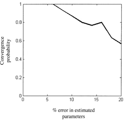
Figure 4 below shows a plot containing the error's of estimated parameters in percent along the x versus the probability of convergence of the LQR controller on the y axis; for statistical sample sizes of 30. What this chart effectively shows is that the LQR gains work as if they were ideal until the estimated parameter value errors become about 6%. The data shown in figure 3 showed an estimated error of around 5% maintaining a theoretical 100% probability of convergence on the LQR controller within its basin of attraction even with the non-ideal parameter updates.

1 0.8 -> .6 0.4 0.2 -0II I 0 5 10 15 20 % error in estimated parameters

Figure 4: Plot showing the errors of estimated parameters in percent along the x versus the probability of convergence of the LQR controller; for a statistical sample size of 30.

Results

The overall results of the effort were positive but there are definitely

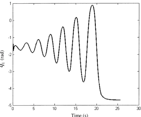
optimizations that can be made with this approach and during the course of the project some possible improved methods were revealed. As can be seen in the state trajectory of Figures 5-8, the system is able to converge marginally well. It is pretty clear in the plots that the LQR controller kicks in around 22 (s) and only requires some small corrections to get the system onto a stabilization trajectory.

0 5 10 15 20 25 30

Time (s)

Figure 5: Trajectory of qi for a successful capture (time versus angular displacement) 10 15 Time (s) Figure 6: Time versus angular 20 25 30

trajectory of the first derivative of qi for a successful capture (time rate).

-0.4

--0.68

-0 .8I I I

0 5 10 15 20 25 30

Time (s)

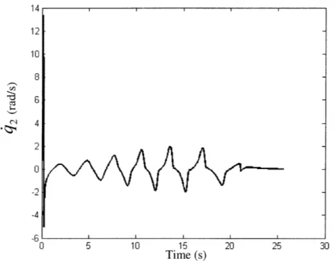
Figure 7: Time trajectory of qz for a successful capture (time versus angular displacement.) 14 12 10 8 23 Cl 4 0 -2 -4 -6 0 5 10 15 20 25 30 Time (s)

Figure 8: Time trajectory of the first derivative of q2 for versus angular rate.)

In 32 of 180 trials from random initial conditions the entire system managed to swing up. This is a 22% success rate which seems acceptable with the implemented modest torque limits and now seemingly naive swing up controller.

Looking back over the project the parameter estimation worked very well, the swing up controller worked well by itself and the LQR controller necessarily worked given the initial conditions were within the basin of attraction of the discrete time, torque limited system. The biggest hole in the approach was the transition between the swing up controller and the LQR stabilizer. All that the swing up controller was trying to

accomplish was to continuously pump energy into the system. This only works well if the controller pumps the correct amount of energy into the system such that it enters the basin of attraction of the LQR system. The majority of the random initial condition trials

were plagued by a swing just under the energy of the LQR basin, followed by a swing just over the energy of the LQR basin. Giving the swing up controller more knowledge of

its goal once it was close would have been a huge improvement here.

It still seems prudent to use this swing up controller when the acrobot is beginning to swing up because this is when parameter estimates are poor and energy based swing up methods would be prone to getting stuck in in-escapable loops near the stable equilibrium state.

Another thing that would have made the problem easier but less interesting would be to allow much higher torques in the LQR controller. With sufficient torque an LQR controller can even power its way through a non-linear region to balance. An attempt that I used to find a basin of attraction of the LQR controller was to store the entrance state into the LQR stabilizer for both the cases when the system failed and when it managed to converge well. Using a least squares parameter estimation technique similar to the one used to estimate the dynamic parameters I was able to obtain the following Equations 56 and 57 for if the system was in the basin of attraction of the LQR controller

all((q,*, 4,, q2, 2 )< 0.4) (56)

Given a large number of trials this method would never give any false positives, and would only give false negatives around 30% of the time. Unfortunately, the swing up controller would almost never get the system into the regime required for these

convergence criteria.

Conclusion

This thesis implements an online, adaptive swing-up and balancing controller with no previous knowledge of the system's mass or geometric parameters. A least squares method then successfully identifies the 5 parameters necessary to completely characterize acrobot dynamics. Swing up is accomplished using partial feedback linearization and a pump up strategy to add energy to the system. The controller then

22% of the time catches the swung up system in the basin of attraction of an LQR controller computed using the estimated parameter values generated from the online system identification.

References

[1] Slotine, J., Li, W., Applied Nonlinear Control, Prentice-Hall, Inc., New Jersey, 1991 [2] Spong, M.W., "Swing Up Control of the Acrobot," 1994 IEEE Int. Conf

on Robotics and Automation, pp. 2356-2361, San Diego, CA, May, 1994.

[3] Araki, N.; Okada, M.; Konishi, Y.; Ishigaki, and H.;. "Parameter identification and swing-up control of an acrobot system." International Conference on International Technology, 2005.

[4] Asada, H. "2.160 Identification, Estimation, and Learning: Lecture Notes No. 2: February 9, 2009". Department of Mechanical Engineering, MIT 2009