HAL Id: hal-02167682
https://hal.inria.fr/hal-02167682
Submitted on 28 Jun 2019HAL is a multi-disciplinary open access
archive for the deposit and dissemination of sci-entific research documents, whether they are pub-lished or not. The documents may come from teaching and research institutions in France or
L’archive ouverte pluridisciplinaire HAL, est destinée au dépôt et à la diffusion de documents scientifiques de niveau recherche, publiés ou non, émanant des établissements d’enseignement et de recherche français ou étrangers, des laboratoires
Wavelength Defragmentation for Seamless Migration
Brigitte Jaumard, Hamed Pouya, David Coudert
To cite this version:
Brigitte Jaumard, Hamed Pouya, David Coudert. Wavelength Defragmentation for Seamless Migration. Journal of Lightwave Technology, Institute of Electrical and Electronics Engineers (IEEE)/Optical Society of America(OSA), 2019, 37 (17), pp.4382-4393. �10.1109/JLT.2019.2924914�. �hal-02167682�
Wavelength Defragmentation for Seamless Migration
Brigitte Jaumard1, Hamed Pouya1, and David Coudert2
1Department of Computer Science and Software Engineering, Concordia University,
Montreal (QC) Canada
2Université Côte d’Azur, Inria, CNRS, I3S, France
June 28, 2019
Abstract
Dynamic traffic in optical networks leads to spectrum fragmentation, which significantly reduces network performance, i.e., increases blocking rate and reduces spectrum usage. Tele-com operators face the operational challenge of operating non-disruptive defragmentation, i.e., within the make-before-break paradigm when dealing with lightpath rerouting in wave-length division multiplexed (WDM) fixed-grid optical networks.
In this paper, we propose a make-before-break (MBB) Routing and Wavelength Assign-ment (RWA) defragAssign-mentation process, which provides the best possible lightpath network provisioning, i.e., with minimum bandwidth requirement. We tested extensively the models and algorithms we propose on four network topologies with different GoS (Grade of Service) defragmentation triggering events. We observe that, for a given throughput, the spectrum usage of the best make-before-break lightpath rerouting is always less than 2.5% away from that of an optimal lightpath provisioning.
Keywords: Wavelength Defragmentation, Seamless Defragmentation, Make-Before-Break Rerouting, Routing and Wavelength Assignment, Fragmented Network, Network Reconfig-uration.
1
Introduction
Software Defined Optical Networks (SDONs) can facilitate automation of complex network oper-ations that result in the flexible deployment of new services in order to meet changing application requirements [1]. Due to the fact that the lightpaths are set up and torn down more frequently in SDONs, they are likely to become fragmented. This fragmentation leads to the circumstance in which new requests face a higher blocking probability even though there is enough capac-ity to satisfy a demand. Spectrum defragmentation operations can reduce lightpath blocking probabilities from 3% [2] up to 75% [3].
A threefold increase expectation for IP traffic by 2021 [4] is also an evidence of the need for an efficient use of the resources in optical networks. Therefore, it is important to regularly reroute the established connections in order to optimize the usage of network resources.
While network reconfiguration is used to refer to different problems, e.g., bandwidth (spec-trum) defragmentation in elastic optical networks [5, 6] or capacity recovery in fragmented Multi-Protocol Label Switching (MPLS) networks by rerouting Label Switched Paths (LSPs) [7, 8], we focus on wavelength defragmentation problem in this study.
Wavelength defragmentation, consists of three phases [9]: (i) decide when to conduct a defragmentation [10]; (ii) design a new lightpath provisioning with a given optimization objective
(e.g., minimum bandwidth requirement) for a given traffic pattern, to ensure the most seamless migration possible; and (iii) migrate from the current lightpath fragmented provisioning to the new optimized one, as seamlessly as possible. The focus of our paper is primarily on the third phase, while its difficulty depends on the previous ones. This study deepens the previous study [11] on the characteristics of a fragmented optical network and the difficulty to defragment it with the paradigm of make-before-break. In particular, we investigate the deterioration of the GoS (Grade of Service, i.e., the number of granted requests) until we reach a steady state, i.e., a worst case scenario for defragmentation with dynamic traffic. We also examine the impact of topology connectivity and the percentage of shortest paths in optimal provisioning on the ease of make-before-break defragmentation.
In the context of wavelength defragmentation, a defragmentation scheme that requires no disruption corresponds to an make-before-break (MBB) reachable wavelength provisioning, i.e., such that we can move from a fragmented wavelength provisioning to an optimized one with the make-before-break process. Within that context, optimized provisioning is such that it drastically reduces bandwidth requirements, ideally with the smallest possible number of re-routings. Deciding whether there exists an MBB defragmentation from a current fragmented provisioning to an optimized pre-computed one by rerouting on-going connections one after the other can be done in polynomial time [12]. An MBB defragmentation can be defined using a Move-To-Vacant (MTV) algorithm, i.e., sequentially choosing a connection, finding a new path using spare resources and then switching the connection to its new path. The process goes on until the new state of the network satisfies the desired constraints, e.g., overall usage of resources or no vacant path is found for any of the demands [13].
In the wavelength defragmentation problem studied in this paper, we aim to find an optimal provisioning for a set of lightpaths such that it can be reached from the current fragmented provisioning with no disruptions (MBB).
The paper is organized as follows. Section 2 is devoted to literature review on wavelength defragmentation and Routing and Wavelength Assignment (RWA) provisioning algorithms. In Section 3, we propose a defragmentation framework in order to investigate the make-before-break wavelength defragmentation problem. Section 4 proposes a nested decomposition optimization algorithm, called wdf_ncg (Wavelength DeFragmentation - Nested Column Generation), that computes the minimum bandwidth RWA provisioning that is reachable with make-before-break. Section 5 describes the details of the wdf_ncg algorithm, which adopts a nested decomposition scheme. Therein, we also propose two other algorithms, one for reducing the size of the depen-dency graph that records the rerouting ordering of the connections, and one to speed up the restoration of the feasibility conditions at each iteration of the wdf_ncg algorithm. Extensive numerical results are presented in Section 6.
2
Literature Review
We first review the studies on WDM network defragmentation, and then the recent work on RWA provisioning as our proposed algorithms for wavelength defragmentation will borrow some of their ideas.
Note that there are also many references on spectrum or flexible reconfiguration, and in particular on defragmentation, in the context of the Routing and Spectrum Allocation (RSA) problem for flexible optical networks [14, 15]. We omit them as there are not relevant for the WDM network defragmentation problem studied in this paper, as well as for the models and algorithms we propose.
2.1 WDM Network Defragmentation
Network defragmentation can be defined as the process of finding out when and how to migrate to a new configuration with a minimum number of disruptions [9]. Network defragmentation may be required in an optical network due to a change in traffic demand, a failure in the network, a change in the network topology or some maintenance operations [16]. Every network defragmentation process consists of three phases as described in the introduction.
For the first phase, i.e., when to trigger a defragmentation, several performance metrics [9] exist, e.g., the average length (number of links) of the lightpaths, the capacity of the alternative routes, the denial of a new incoming connection.
The second phase consists in building an optimized lightpath provisioning. We review in Section 2.2 the key models and algorithms of the literature. An alternate option would be to directly build the best possible optimized provisioning that can be reached without any disruption. While this has been studied a lot with heuristics, which do not provide any information on how far is their solution from the best possible one, we are aware of only one study with an exact model and algorithm in the context of layer 2 (MPLS) defragmentation, i.e., [7].
The third phase that defines the order of the rerouting so that the migration is completely seamless or as seamless as possible, has been studied with different objective functions, e.g., minimizing the total number of disruptions [17], minimizing the maximum number of concurrent disruptions [12, 18], minimizing disruption time [17] and minimizing defragmentation costs [19]. A comparison of the first two objective functions can be found in [20].
Seamless WDM network defragmentation mean make-before-break defragmentation and we can create it in two different ways. The first way, i.e., the 2-step way as discussed above, is as follows: given the fragmented provisioning and the optimized one, define the best rerouting order so as to define a seamless migration if one exists, or the most seamless possible one. The second way, i.e., a progressive method, is to reroute one connection at a time with, e.g., a MTV algorithm, in order to minimize the bandwidth requirements, until we cannot reduce them fur-ther. Drawback of the 2-step way is that very often, no incentive is considered for reducing the number of reroutings when computing the optimized provisioning. Consequently, it often leads to an optimized (e.g., smaller bandwidth requirement or less blocking) provisioning at the expense of a larger number of connections to reroute. Drawback of the progressive way is that it is often considered with the help of heuristics and therefore no information is available on how far is the resulting provisioning from an optimized (MBB) one.
Seamless wavelength defragmentation has been studied in [21]. They propose a heuristic based on greedy randomized adaptive search procedure (GRASP). Their GRASP algorithm returns the best MBB provisioning that can be found within the limit of a given number of iterations. Other authors consider wavelength defragmentation with the minimum number of disruptions, i.e., minimum lightpath disruptions. An Integer Linear Programming (ILP)-based wavelength defragmentation solutions for optimizing wavelength resource utilization with min-imal optical path disruptions during the migration process is proposed in [22]. They evaluate their method under a computation time limitation of 10 minutes. The proposed approach can improve the resource efficiency of 20% on sample metro networks Japan Photonic Network (JPN) with 48 nodes, 91 bidirectional links and 100 lightpaths. Different heuristics are proposed in [23] to minimize the disruptions of system resources (transmitters/receivers) while migrating between two given configurations. They define a benefit associated with each lightpath, e.g., transmission delay or number of conflicts with old lightpaths. They propose different heuristics based on the benefit of a lightpath, e.g., using the same benefit or updating the benefits of remaining unestablished lightpaths. They compare the performance of their heuristics
accord-ing to the computational times and the number of resource disruptions. The heuristic usaccord-ing the number of conflicts as the benefit of a lightpath yields the minimum number of disrupted transceivers.
All reviewed papers in the literature (except [22]) study heuristics and the largest size in-stances solved so far are related to a NSFNET network with 16 nodes, 25 links and 140 lightpaths [23], and the GEANT2 network (33 nodes, 46 links and 1,000 lightpaths) [21].
While network defragmentation with a minimum number of disruptions is certainly of interest in the context of the Internet, most optical network carriers only consider seamless WDM network defragmentations due to the Service Level Agreements with their customers. Consequently, our objective is to investigate how to build the minimum MBB bandwidth lightpath provisioning for a given defragmentation event, with an exact algorithm.
2.2 Routing and Wavelength Assignment
In order to design an efficient wavelength defragmentation algorithm, it is important to review the best models and algorithms for the RWA provisioning, i.e., defining routes and assigning wavelength to these routes [24]. Studies on RWA provisioning differ in their assumptions and objective functions. The most common objective functions are the maximization of the GoS or equivalently minimizing the blocking rate (max-RWA) [25, 24] and the minimization of the required bandwidth (min-RWA) [26, 27]. RWA has also been widely studied for static (the entire set of connections is known in advance) and dynamic cases (a lightpath is set up for each connection request as it arrives) [24, 28]. It has been shown in the literature that static RWA is NP-complete [29].
While many heuristics have been proposed to solve the RWA problem [30], significant progress has been made with exact algorithms, allowing to solve exactly the RWA problem for large instances, i.e., networks with up to 90 nodes and 150 wavelengths, and traffic between all node pairs [24].
3
WDM Network Defragmentation Problem: Our Framework
We present here an overview of the WDM network defragmentation framework we use in order to investigate the MBB wavelength defragmentation problem. It includes three steps, which are detailed below.
3.1 WDM Network Defragmentation Framework
We assume we are given a WDM optical network, and that the input of our WDM network defragmentation framework is a demand given by a set of connections. Each connection, if granted, is to be provisioned by a lightpath, i.e., the combination of a route and a wavelength, the same one (so-called continuity constraints) all the way from the source to the destination. The framework we propose is as follows.
Initialization:
Compute a maximum GoS RWA provisioning, i.e., grant the largest possible number of con-nections.
Step 1: Dynamic RWA Provisioning Repeat
Free the resources of each terminating connection.
Grant each new incoming connection if there are spare resources to provision it, and else deny it.
Until a wavelength defragmentation is triggered Step 2: Trigger Defragmentation
When the deterioration of the GoS reaches a given threshold, trigger defragmentation. Let RWAfrag be the resulting RWA provisioning.
Step 3: Conduct Defragmentation
Step 3.1. Compute RWAopt, a minimum bandwidth RWA provisioning
Step 3.2. Initialize RWAmbb_opt, an MBB reachable RWA provisioning with RWAopt
If RWAmbb_opt is MBB reachable from RWAfrag
Reroute one request at a time with the MBB technique Return to Step 1
Else
Identify some rerouting deadlocks (i.e., conflicting rerouting order such as k needs to be rerouted before k0 and vice-versa)
Recompute a minimum bandwidth RWA provisioning with the deadlock avoidance con-straints
Let RWAmbb_opt be the new optimized RWA provisioning
Return to Step 3.2.
Figure 1 illustrates our WDM network defragmentation framework. For every incoming request, we check whether there are available spare resources to grant it, even if it means routing it on a longer route. In other words, we search for the shortest lightpath that is available considering the current spare resources. If no spare resource is available, the connection is denied, otherwise it is granted. Better granting proactive algorithms are possible, especially when information is available on the future/forecast traffic, but as this is not the focus of this study, we use the simplest rule for granting connections. Hence, for every new connection request we solve a dynamic max-RWA problem. For every ending connection, the resources used by the corresponding lightpath are freed and made available for future traffic.
3.2 Triggering of the Wavelength Defragmentation
While it goes beyond the scope of this paper to investigate the best way to trigger wavelength de-fragmentation, we made sure that the way we choose did not facilitate or worsen the wavelength defragmentation, especially under the make-before-break paradigm.
Different performance metrics have been proposed in the literature, see, e.g., [9] for a recent survey on them. We decided to use the Grade of Service (GoS) as the triggering event and, as we will see in the numerical results (see Section 6), we use different threshold GoS values, from restrictive ones (e.g., a GoS decrease of 5%) to more permissive ones (up to 50%). We also observe that, without wavelength defragmentation, the stabilization of the GoS is reached at various levels, depending on the network topologies (all experiments were done with uniform traffic), see Section 6.
3.3 min vs. max RWA provisioning
Throughout the WDM network defragmentation framework, we deal with two variants of the RWA problem: Dynamic Max-RWA in the dynamic provisioning phase and Static Min-RWA in the wavelength defragmentation phase. We briefly remind their definitions in what follows.
3.3.1 Static Min-RWA
In static RWA, the set of requested connections D is known. The objective function is to grant all connection requests while minimizing the bandwidth requirements over a multigraph
Dynamic routing phase of granting/denying of connections on spare resources time Performance metric, e.g., Throughput Defragmentation events Throughput threshold Granted incoming connection Denied incoming connection Terminating connection
…
…
…
…
…
…
…
…
…
…
…
Figure 1: WDM Network Defragmentation Process
G = (V, L) with V (indexed by v) and L (indexed by `) representing the set of nodes and links ofG, respectively. D = (Dsd)(vs,vd)∈SDdefines the number of requested unit lightpaths for every
node pair with traffic, i.e., (vs, vd) ∈ SD ⊆V × V . Each granted connection unit is assigned
a lightpath (p, λ) where p is a routing path and λ is the selected wavelength among the set of available wavelengths Λ. No two lightpaths using the same link can share the same wavelength (under the assumption of a single directional fiber in each direction for connected node pairs).
3.3.2 Dynamic Max-RWA
In the dynamic max-RWA problem, the objective function is to grant the largest possible number of connections (GoS) or equivalently to minimize the blocking rate. The set of demands are not known in advance. There is a set of legacy (i.e., on-going) connections Dlegacy routed on a
multigraph G = (V, L) and a set of new incoming demands Dnew. We need to assign available
lightpaths toDnew such that no wavelength conflict occurs. Interested reader may refer to, e.g.,
[24] for detailed formulation in both dynamic and static cases of RWA. In the particular case of one new incoming connection to provision at a time, the dynamic max-RWA problem amounts to searching for an available shortest path connecting the two endpoints of the connection.
4
A Nested Decomposition Wavelength Defragmentation
Algo-rithm
In this section, we assume that an optimized RWA provisioning, called RWAopt, is available.
We then aim at designing a model (called wdf_mbb) and an algorithm (called wdf_ncg) that will modify RWAopt as little as possible so that it can be reached with make-before-break
One of the key elements of the wdf_ncg algorithm is the so-called dependency graph. It is introduced in the next section. The second key element is the computation of a RWA provisioning subject to rerouting deadlock avoidance constraints. Consequently, we reviewed all the previous scalable mathematical models for RWA and selected the most relevant one for designing the wdf_mbb model, see Section 4.3. Section 4.4 describes the wdf_ncg algorithm, which is an iterative algorithm alternating solution of the wdf_mbb model and identifying rerouting deadlocks with the dependency graphs, until reaching a minimum bandwidth MBB reachable RWA provisioning.
4.1 Dependency Graph and Lightpath Rerouting Order
In order to define the order in which the lightpaths can be rerouted, we build the so-called dependency graph Gd = (Vd, Ld), introduced in [31], between the fragmented (RWAfrag) and
the optimized (RWAopt) provisionings at the end of each defragmentation interval (see Figure
2(c)). A dependency graph is a directed graph that represents the dependence between rerouted requests. Node and link sets of the dependency graph are defined as follows.
Vd= {π = (p, λ) : π is a lightpath in RWAfrag}
Ld= {(π, π0) :π0 needs to be rerouted before π in order to reach RWAopt with MBB}.
In other words, each link (π, π0) defines the order of migration between two lightpaths, when a lightpath π0 needs to be rerouted before another lightpath π in order to perform an MBB rerouting.
Figure 2 illustrates an example on how to build a dependency graph. As mentioned before, dependency graph is built based on two different provisionings. In Figure 2(a) a fragmented provisioning (RWAfrag) with 29 used links is represented while Figure 2(b) shows an optimized
provisioning (RWAopt) for the same set of demands with 21 used links. Figure 2(c) is the
dependency graph built based on the provisionings presented in Figures 2(a) and 2(b). Every link in the dependency graph shows one dependency and the right order of rerouting lightpaths. For example, lightpathπ1in RWAoptis routed over blue wavelength and has three links (v3→ v6,
v6 → v5 andv5 → v4) in common with lightpathπ4 in RWAfrag. This means that lightpathπ4
needs to be rerouted first in order to make room for lightpath π1 in RWAopt. In other words,
lightpathπ1 cannot be rerouted before lightpathπ4is rerouted. This dependency (also rerouting
order) is represented by a link from vertex π1 to vertex π4 in the dependency graph. Table 1
shows all the dependencies in this migration. There is one link in the dependency graph for every dependence presented in Table 1. It should be mentioned that lightpath π7 has the same
wavelength and the same path in both RWAfragand RWAopt, hence, it has no dependency and
does not appear in the dependency graph.
We use Algorithm 1 to build the dependency graph (Gd= (Vd, Ld)) between RWAfrag and
RWAopt.
For a given lightpath, denote by πifrag and πopti the lightpath in the fragmented and in the optimized provisioning respectively.
After building the dependency graph, we need to determine the rerouting order of the light-paths. Since the path and the bandwidth required for the lightpaths with no dependency (no outgoing link), i.e., lightpath π2 in Figure 2(c), are already available in RWAopt, they are first
rerouted. After each rerouting, at least one link in the dependency graph is removed and it might result in one or more lightpaths with no dependency, e.g., lightpathπ3 can be rerouted sinceπ2
Table 1: List of dependencies
Lightpath Rerouting dependence(s) Common links
π1 π4 v3 → v6,v6→ v5,v5 → v4 π2 - -π3 π2 v8 → v9,v9→ v6,v6 → v3 π4 π5 v3→ v2 π8 v2→ v1 π5 π3 v8 → v5,v5→ v2 π6 π9 v5→ v4 π8 π1 v2 → v1,v1→ v4 π9 π6 v5 → v8,v8→ v7
v
1
v
2
v
3
v
4
v
5
v
6
v
7
v
8
v
9
π1 wavelength λ1 π2 π3 π4 wavelength λ2 π5 π6 π7 π8 π9(a) Fragmented provisioning RWAfrag
v
1
v
2
v
3
v
4
v
5
v
6
v
7
v
8
v
9
π1 π2 π3 π4 π5 π6 π7 π8 π9(b) Optimized provisioning RWAopt
π
1
π
2
π
3
π
4
π
5
π
6
π
8
π
9
(c) Dependency graph for RWAfrag→ RWAopt
Figure 2: An Example of Dependency Graph
Algorithm 1 Dependency Graph Builder
1: Input: Network Topology, RWAfrag, RWAopt
2: Output: Dependency Graph Gd= (Vd, Ld)
3: Vd← ∅; Ld← ∅
4: for ∀ lightpathπopti with a different routing than πfragi do
5: Vd← Vd∪ {πi} 6: for every link` ∈ L do
7: for every lightpathπopti using link` do
8: if there is a lightpath πjfrag using link` such that λπopt i =λπ frag j then 9: add arc (πi, πj) toLd 10: ReturnGd= (Vd, Ld)
π3 is rerouted. For the remaining lightpaths, since they are involved in a circuit (a rerouting
deadlock), they all have dependencies and rerouting each one requires at least one disruption. As seen in the dependency graph (Figure 2(c)), there are 2 circuits, one involvingπ1,π4 andπ8
and the other involvingπ6 andπ9. Hence, if we want to build an MBB provisioning, we need to
identify the circuits and prevent them from occurring again. Since maximal link disjoint circuits are easily identifiable once we have computed strongly connected components, we will proceed with the computation of strongly connected components, using the algorithm of Tarjan [32].
4.2 Identification of Avoidable Disruptions: Reducing the Number of Cir-cuits in the Dependency Graph
In this section, we propose an algorithm in order to check whether it is possible to break some of the circuits without adding cuts and compromising the optimal solution by finding new lightpath(s) for one or some of the connections. Figure 3 represents an example of removing a circuit by finding a new lightpath for π1. As seen in Figure 3(c), there is a circuit involving
π1 and π2 while migrating from the fragmented provisioning (Figure 3(a)) to the optimized
provisioning (Figure 3(b)). If we can find a new lightpath for one of these connections without creating new circuits, then a seamless migration will be possible. As seen in Figure 3(d), a new lightpath can be assigned to lightpath π1 that not only does not create a new circuit but also
breaks the circuit between π1 and π2. It should be mentioned that it is also possible to find a
new lightpath forπ2 and get the same results, e.g., changing the wavelength of π2 from blue to
red on the same path in Figure 3(d) returns the same result that is an MBB provisioning.
v
1
v
2
v
3
v
4
v
5
v
6
v
7
v
8
v
9
π1 π2 π3 π4 π5 π6(a) Fragmented Provisioning
v
1
v
2
v
3
v
4
v
5
v
6
v
7
v
8
v
9
π1 π2 π3 π4 π5 π6 (b) Optimized Provisioningπ
1
π
2
(c) Dependency graphv
1
v
2
v
3
v
4
v
5
v
6
v
7
v
8
v
9
π1 π2 π3 π4 π5 π6(d) Revised Optimum Provisioning
Figure 3: Preprocessing Operation
In Algorithm 2, after building the dependency graph Gd and finding the set C of Strongly Connected Components (SCCs), we try to find for each lightpath involved in a SCC a new
lightpath, of the same length, that allows the break of a circuit in the SCC and eventually make it acyclic. If such a new lightpath is found for a given connection request, we use it and update Gd accordingly. We repeat this process untilGd becomes acyclic or we can no longer find any new lightpath helping to break circuits. If there are no more circuits, it means that an MBB provisioning has been found. But, finding no lightpaths to be rerouted while there are still some circuits shows that Algorithm 2 cannot break any other circuits and so that a seamless migration is not yet possible.
It should be mentioned that the nodes in Gd are prioritized based on their in-degree (the number of arcs ending in each node). The reason is that having higher in-degree for a given lightpathπ shows that more lightpaths are dependent on π and it can contribute to more circuits.
Algorithm 2 Preprocessing Algorithm Input: Dependency graph Gd
Input: Gλ = (V, Lλ) ⊆ G = (V, L) where Lλ is the set of links which are not used in any
lightpath usingλ, for λ ∈ Λ.
Output: New wavelength assignment for some lightpaths involved in circuits
1: Find the strongly connected components (SCCs) ofGd
2: Build the list Π of lightpaths, i.e, the set of nodes inGd, involved in the SCCs
3: Sort Π by non-increasing in-degree inGd
4: for every node (lightpath)π = (p, λ) ∈ Π such that p : vs vddo
5: for everyλ0∈ Λ do
6: p ← shortest path from vˆ s to vd inGλ0
7: if ˆp 6= ∅ and |ˆp| ≤ |p| then
8: Check if changingπ to (ˆp, λ0) creates new circuits inG d
9: if no new circuit is generated then
10: Setπ = (ˆp, λ0) ; UpdateGλ andGλ0
11: Go to step 1
12: return Set of lightpaths
4.3 wdf_mbb Model
As seen in Section 2.2, RWA problem has been widely studied and there are several exact solu-tion schemes in the literature including compact and decomposisolu-tion formulasolu-tions. Although the compact formulations are not scalable, real size instances can be solved exactly using decompo-sition methods, e.g., column generation technique. According to the recent RWA studies [24], the most efficient decomposition is to generate wavelength plans (i.e., set of pairwise link disjoint lightpaths using the same wavelength) using a path formulation, followed by a link formulation in order to guarantee the optimality of the linear relaxation of the model.
In order to avoid the use of a link formulation, which is computationally costly to solve, we propose to use a nested decomposition scheme. We first establish the so-called master problem of the decomposition scheme, called wdf_mbb model. We will next discuss its detailed solution in Section 5.
The wdf_mbb model relies on the concept of wavelength configurations, where a config-uration γ corresponds to a wavelength plan, for a given wavelength λ. While in the RWA decomposition models, configuration (i.e., wavelength plan) can be defined for a generic wave-length and therefore do not have any symmetry issues (the wavewave-length assignment is done a posterior), this is unfortunately not possible here in order to be able to express the rerouting deadlock avoidance constraints.
Model wdf_mbb requires one unique set of decision variables zγ for γ ∈ Γ. Each variable
zγ allows or not the selection of configurationγ in the optimal RWA provisioning output.
Each configurationγ ∈ Γ is formally defined by the following parameters:
Bγ = bandwidth requirement of configurationγ, as expressed by the number of links used in γ
for routing some connections
aγsd= number of lightpaths for node pair (vs, vd) in configurationγ
aγπ = 1 if lightpathπ is used in configuration γ, 0 otherwise.
We now express the wdf_mbb model that computes the minimum bandwidth RWA provi-sioning subject to deadlock avoidance constraints as identified in the dependency graph. Since the number of circuits in a directed graph can be exponential, we do not introduce all possi-ble circuits. Using Tarjan’s algorithm, we identify the strongly connected components (SCCs). While a SCC can contain several circuits, we add only one circuit per SCC in order to control the number of constraints, i.e., the circuit that includes all nodes of the SCC.
Minimize: X γ∈Γ Bγzγ (1) Subject to: X γ∈Γλ zγ ≤ 1, λ ∈ Λ (2) X γ∈Γ aγsdzγ ≥ Dsd, (vs, vd) ∈ SD (3) X π=(p,λ)∈c X γ∈Γλ aγπzγ ≤ |c| − 1 c ∈ C (4) zγ∈ {0, 1}, γ ∈ Γ. (5)
Constraints (2) ensure that we select at most one configuration for each wavelengthλ. Con-straints (3) enforce the demand conCon-straints, with the left-hand side term computing the number of demand units provided by each configuration, and then summing over all configurations. Constraints (4) guarantee that the provisioning will not contain any of the circuits c ∈ C. Constraints (5) define the domains of the variables.
4.4 wdf_ncg Algorithm
In order to find an MBB provisioning, we propose an iterative process presented in Algorithm 3. This process starts with building a dependency graph Gd for migrating from a fragmented provisioning (RWAfrag) to an optimized provisioning (RWAopt). Tarjan’s algorithm is used in
order to find the set of circuitsC (strongly connected components) in Gd. Algorithm 2 helps us break some of the circuits. If C is empty, it means that a seamless migration has been found. Otherwise, one constraint corresponding to each circuit c ∈ C is added to wdf_mbb. The solution of wdf_mbb is the updated RWAopt that does not contain any of the circuits found
in previous iterations due to deadlock avoidance constraints. However, it may contain some new circuits. Hence, the dependency graph is generated, set of circuits are found and Algorithm 2 tries to reduce the number of circuits in C. This process goes on until the set of circuits C is empty.
Algorithm 3 wdf_ncg Algorithm Input: RWAfrag, RWAopt
Output: make-before-break RWAopt
1: Build dependency graphGd (Algorithm 1).
2: Find the set of circuitsC in Gd (Tarjan’s Algorithm).
3: Reduce the number of circuitsC (Algorithm 2).
4: whileC is not empty do
5: Update RWAopt by solving wdf_mbb
6: Build dependency graph Gd(Algorithm 1).
7: Find the set of circuits C in Gd (Tarjan’s Algorithm).
8: Reduce the number of circuitsC (Algorithm 2).
9: return RWAopt
5
Solution the wdf_mbb Model: A Nested Decomposition
Wave-length Defragmentation Model
We first discuss the details of the solution process for the wdf_mbb model with a nested decomposition algorithm in Section 5.1. We next discuss in Section 5.2 an algorithm in order to speed up the feasibility in wdf_mbb model after the addition of new rerouting deadlock avoidance constraints.
5.1 Nested Column Generation
The wdf_mbb model proposed in Section 4.3 has an exponential number of variables, and therefore is not scalable if solved using classical ILP (Integer Linear Programming) tools. Indeed, we need to use column generation techniques in order to manage a solution process that only requires an implicit enumeration of the wavelength configurations (interested readers may refer to Chvátal [33]). Column generation method allows the exact solution of the linear relaxation of model (1)-(5), i.e., where variables zγ ∈ Z+ are replaced by zγ ≥ 0, for γ ∈ Γ. It consists in
solving alternatively a restricted master problem (the wdf_mbb model in Section 4.3 with a very limited number of columns/variables) and the pricing problem (generation of a new wavelength configuration) until the optimality condition is satisfied (i.e., no wavelength configuration with a negative reduced cost). In other words, when a new wavelength configuration is generated, it is added to the current restricted master problem only if its addition implies an improvement of the optimal value of the current restricted master problem. This condition, indeed an optimality condition, can be easily checked with the sign of the reduced cost, denoted by cost, see (6) for its expression (the reader who is not familiar with linear programming concepts is referred to [33]), of variables zγ.
Once the optimal solution of the LP (Linear Programming) relaxation (z?
lp) has been reached,
we solve exactly the last restricted master problem, i.e., the restricted master problem of the last iteration in the column generation solution process, using a branch-and-bound method, leading then to anε-optimal ILP solution (˜zilp), whereε = (z?
lp− ˜zilp)/zlp? . Branch-and-price methods
can be used in order to find optimal solutions, if the accuracy (ε) is not satisfactory, see, e.g., [34].
In order to solve wdf_mbb, we design a nested column generation algorithm in which each pricing problem is solved by column generation itself. In other words, the master problem comprises all generated wavelength configurations. Each wavelength configuration is a set of feasible link disjoint paths and first level pricing problem is responsible for generating such
configurations.
Each wavelength configuration (first level) pricing problem can be viewed as a second level master problem and a set of second level pricing problems. Each second level pricing problem generates a path for a given node pair (vs, vd) ∈ SD. The objective in the second level master
problem represents the cost of the wavelength configuration in the current pricing problem. We now present the second level master and pricing problems.
We first introduce the set of variables: βsd
p = 1 if pathp is used in the wavelength configuration under construction, 0 otherwise.
Note that γ is omitted in the sequel in order to alleviate the notations (e.g., Bγ B). Let
Πcλ be the set of lighpaths in c using λ.
min costconfig=B − u(2)λ − X (vs,vd)∈SD X p∈Psd βsd p u (3) sd −X c∈C X (vs,vd)∈SD X p∈Psd:π=(p,λ)∈Πcλ u(4)c βpsd (6) subject to: X (vs,vd)∈SD X p∈Psd δ`pβpsd≤ 1 ` ∈ L (7) X p∈Psd βsd p ≤ Dsd (vs, vd) ∈ SD (8) X (vs,vd)∈SD X p∈Psd X `∈L δ`pβsd p ≤ B (9) βsdp ∈ {0, 1} (vs, vd) ∈ SD, p ∈ Psd, (10)
whereδ`p is equal to 1 if link ` belongs to path p.
Constraint set (7) assures that selected paths are link disjoint. Thanks to constraint set (8), no more than Dsd is granted for every node pair (vs, vd) ∈ SD. Constraint set (9) determines
the number of used links in current configuration. Observe that for a pathp ∈ Psd,P`∈Lδ p ` is
the length of pathp.
In order to generate a path between a given node pair (vs, vd) ∈ SD, we find the path with
minimum cost in the second level pricing problem:
min costpath= −u(3)sd −
X `∈L δ`u (7) ` − u (8) sd − u (9)X `∈L δ`. (11)
If the output path is equal to one of the paths involved in a circuit using wavelength λ, then −u(4)c needs to be subtracted from the reduced cost.
Since u(3)sd andu(8)sd are constant values for a given node pair, objective (11) can be rewritten as
min costpath= − X `∈L δ`u (7) ` − u (9)X `∈L δ` (12)
and will need to be adjusted with the constant terms (−u(3)sd − u(8)sd (−u(4)c )), before checking his
sign. Note that −u(4)c refers to checking whether the output path is equal to one of the paths
inequality constraints that are “≤", and as we have a minimization problem, those dual values are both non-positive. We can then assign a non-negative weight −u(7)` − u(9) to each link and
use a polynomial-time algorithm, e.g., Dikjstra’s algorithm, to find a weighted shortest path for a given node pair for solving the second level pricing problems.
5.2 Re-Establishment of a Feasible RWA Provisioning
We propose Algorithm 4 in order to overcome the infeasibility while obtaining ILP solution, due to the addition of the deadlock avoidance constraints.
Algorithm 4 Building a feasible ILP solution
Input: A feasible LP solution: A set of configurations Γlp Output: A feasible ILP solution: A set of configurations Γilp
1: Γilp= ∅.
2: Sort configurations in LP based on their LP value.
3: forλ ∈ Λ do
4: Choose a configuration γ with max LP value.
5: Γilp= ΓilpS{γ}
6: Update Γilp by removing lightpaths related to overfilled demands (longest lightpaths). See Constraint (3).
7: Update Γilp by removing lightpaths violating the circuit constraints (longest lightpaths).
8: Build the set of unfulfilled demands (Duf).
9: whileDuf is not empty do
10: Choose a demand d ∈ Duf
11: if It is possible to find a lightpathπ satisfying circuit elimination constraints then
12: Assign π to d ; Duf ← Duf − {d}
13: else
14: Find the busiest configuration γ
15: i.e., with the maximum number of lightpaths
16: Free up the shortest path for d in γ by removing a
17: set of lightpaths related to a set of demandsDr
18: Duf ← Duf − d ; Duf ← DufS Dr
return Γilp
6
Computational Results
6.1 Traffic and Network Data Sets
We use four different networks, whose key characteristics (number of nodes and links, average node degrees) are described in Table 2, see [24] for their references.
Table 2: Main characteristics of the networks Networks |V | |L| Avg. node deg. # wavelengths
USA 24 88 3.7 75
GERMANY 50 176 3.5 130
NTT 55 144 2.6 42
Table 3: Statistics for the Characteristics of the Strongly Connected Components (SCC) in the Dependency Graphs
Networks GoS # of nodes in SCC/AVG degree (# Links/# Nodes) # Reduction SCC #1 SCC #2 SCC #3 SCC #4 SCC #5 SCC #6 SCC #7 SCC #8 SCC #9 SCCs NTT 10% 282 2.20 3 2 2 1 2 1 1 0 589 15% 251 2.23 3 1.33 1 0 581 20% 318 2.28 3 3.33 2 3 1 0 445 25% 170 2.46 6 1.83 3 2 3 1.67 3 1.33 2 6.50 2 3 2 1.50 1 0 542 USA 5% 529 2.13 1 0 412 10% 506 2.11 2 3 1 0 387 15% 428 2.11 3 6 2 3 2 1 1 0 413 GERMANY 5% 1,062 2.43 1 0 775 10% 544 2.16 3 2 3 2 2 2.5 1 0 1,190 15% 175 1.65 5 1.60 3 2 2 2 2 1.50 2 1.5 2 1.50 2 1 1 0 1,453 20% 20 1.50 10 1.40 5 1.60 3 2 2 1.50 2 1 1 0 1,413 25% 16 2 1 0 1,446 CONUS 25% 249 2.73 9 2.25 7 2.33 4 2 1 0 469 30% 153 2.31 9 2.44 4 2 2 1 1 0 504 35% 184 2.64 2 4 2 3 2 1 1 0 444
6.2 Generation of Fragmented RWA Provisionings
In order to generate a RWA provisioning, we use the framework described in Section 3. The first initial provisioning corresponds to the RWA provisioning obtained in [24], with the objective of maximizing the Grade of Service (GoS), i.e., the number of granted requests. We then use a dynamic RWA process with add and drop requests, using a random generator such that the probability of add and drop is the same, i.e., 0.5. Source and destination of the add and drop requests are selected at random.
We report the GoS behavior for two networks in Figure 4, where the GoS (left vertical axis) is expressed in % and the right vertical axis reports the number of shortest paths. We plot two sets of curves, the top ones (blue curves) are each associated with one random dynamic traffic and the red curve is the average of the five individual dynamic RWA curves. The second set of curves (bottom ones) corresponds to the number of granted requests on a shortest path (be aware that for a given node pair, there may exist several shortest paths). Again, we have 5 individual curves (orange ones) and one additional curve (green curve) that represents their average.
We observe that the steady state takes a variable number of add and drop requests before reaching a steady state, depending on the networks. In addition, the steady state is reached for different values of GoS. USA (Figure 4(b)) network has a larger GoS value than NTT (Figure 4(a)) in its steady state. An explanatory factor is the average node degree of the networks, see Table 2. Indeed, USA has a higher average node degree, and consequently is more connected. This leads to more options for establishing a lightpath for incoming requests, with the length of routes increasing more slowly. Behavior of the number of requests routed on a shortest path follows the behavior of the GoS decrease, as expected. As the GoS decreases, the network becomes more fragmented and, as a result, fewer shortest paths are available to grant and route incoming requests.
6.3 Reduction of the Number of Rerouting Deadlocks
6.3.1 Distribution and Sizes of the Strongly Connected Components
As mentioned in Section 2.1, network defragmentation is triggered by the GoS. Table 3 shows the different GoS values we considered. For every GoS value, we computed the Strongly Connected
(a) NTT
(b) USA
Figure 4: Fragmented Networks (GoS)
Components (SCCs) of the dependency graph. Therein, SCC#i denotes the ith largest SCC, where the size is measured by the number of nodes in each SCC, i.e., the number of lightpaths in the optical network. If they are all of size one, we can conclude that the optimal RWA provisioning is MBB reachable. However, this was the case for none of the data instances as showed in Table 3: each data instance is such that its associated dependency graph has at least one strongly connected component with a size larger than 1.
We observe that most data instances are such that the dependency graph contains only one strongly connected component with more than one node. In addition, the latter component is usually quite large, as in the theoretical results on the distribution and size of strongly connected components in random graphs, see, e.g., [35].
6.3.2 Reduction of the Number of Rerouting Deadlocks
We report in Table 3 the number and sizes of the strongly connected components after applying Algorithm 2. We observe that the number of strongly connected components has significantly increased as a consequence of the drastic reduction of the size of the largest strongly connected components, still on average larger than one. While seamless migration is still not yet possible for most of the cases except for GERMANY (5% and 25%), the number of rerouting deadlocks, as expressed by the number of circuits, and hence the size and the density of the strongly connected components of size larger than 1, has significantly decreased.
Table 4: Statistics for the SCCs after preprocessing algorithm
Networks GoS
# of nodes in SCC vs.
# Reduction avg node degree (# Links/# Nodes) SCCs
SCC #1 SCC #2 Other SCCs NTT 10% 2 2.50 1 0 0 0 874 15% 20 1.85 1 0 0 0 814 20% 16 2.25 9 2.00 8 6.17 738 25% 3 1.67 3 1.67 7 10 722 USA 5% 4 2.00 4 1.75 5 3 932 10% 24 2.00 1 0 0 0 870 15% 7 1.57 5 1.20 1 0 834 GERMANY 5% 1 0 0 0 0 0 1,836 10% 9 1.45 3 2.00 1 0 1,728 15% 16 1.44 2 1.50 3 1.50 1,621 20% 5 1.60 2 1.50 3 1 1,446 25% 1 0 0 0 0 0 1,453 CONUS 25% 5 3.44 4 1.5 3 2 714 30% 2 1.50 1 0 0 0 667 35% 2 3 2 1.50 1 0 629 represented in Figure 5.
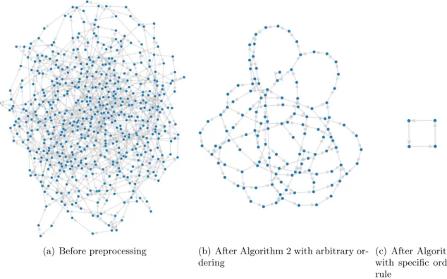
Figure 6 illustrates the efficiency of using the ordering criterion of Algorithm 2 with respect to the in-degree of the nodes of the dependency graph. Indeed, Figure 6(a) represents the strongly connected component of the USA5% data set, after the first construction of the dependency graph. Therein, we can observe many rerouting deadlocks. Figure 6(b) depicts the largest strongly connected component after applying Algorithm 2, using an arbitrary order of the nodes: the size of the largest strongly connected component has significantly decreased, and we can observe a weaker density with several interconnected circuits. Lastly, Figure 6(c) shows again the largest strongly connected component, this time after applying Algorithm 2 with its current ordering rule for node processing. We can note a very significant reduction of the strongly connected component, now limited to a single circuit, i.e., a single rerouting deadlock.
6.4 Seamless or Almost Seamless Wavelength Defragmentation
We now evaluate the compromise to be made on the minimization of the bandwidth requirement in order to get a seamless, i.e., make-before-break, wavelength defragmentation. As described in Section 4.4, the wdf_ncg algorithm searches for alternate wavelength provisioning when a rerouting deadlock is identified in the dependency graph, and it may result in increasing the bandwidth requirements.
We report the results in Table 5. No data instance requires more than 5 rounds of the iterative process of the wdf_ncg algorithm and six instances are solved in 1 round. NTT with threshold 25% requires the largest number of deadlock avoidance constraints, i.e., 11 additional constraints.
In addition, the wdf_ncg algorithm is also pretty much scalable. All 13 instances are solved in less than 4 minutes, with 6 instances with a computational time less than 1 minute. It should be noted that the time reported in Table 5 (column "Time") is related to calculating
Figure 5: Performance of Algorithm 2: Reduction of the size of the biggest strongly connected component.
MBB provisioning and does not include the time required for calculating initial RWAopt that
we have reported in column "Min RWA" (time for solving the RWA problem while minimizing the number of used wavelengths).
Table 5: Performance of the wdf_ncg algorithm
Networks GoS # # Time Min RWA
Reduction Rounds Constr. (sec) (sec)
NTT 10% 4 4 203 1,259 15% 1 1 13 1,291 20% 4 8 168 1,332 25% 5 11 202 1,153 USA 5% 3 8 70 619 10% 2 2 28 450 15% 1 2 15 534 GERMANY 10% 1 2 11 13,158 15% 2 4 14 18,027 20% 1 3 10 18,746 CONUS 25% 3 5 165 2,891 30% 1 1 83 2,827 35% 1 2 70 1,069
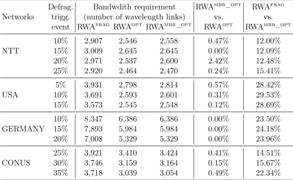
Table 6 provides the bandwidth requirement and how far it is from minimum bandwidth requirement in order to derive a make-before-break reachable wavelength provisioning. We report the bandwidth requirement for the RWAfrag right before the defragmentation event,
the optimal (RWAopt) provisioning and the best wavelength provisioning (RWAmbb_opt) that
is make-before-break reachable. As seen, the difference between link usage of the MBB and optimal provisionings is less than 1% and even equal to the optimal provisioning except NTT (20%) while the performance of the network in terms of used links is improved in all cases.
(a) Before preprocessing (b) After Algorithm 2 with arbitrary or-dering
(c) After Algorithm 2 with specific ordering rule
Figure 6: Largest SCC for USA 5% before preprocessing (6(a)), after applying Algorithm 2 using an arbitrary order of the nodes (6(b)), and after Algorithm 2 with its current ordering rule for node processing (6(c)).
geographical distances presented in [36] for the USA network. As expected, the difference be-tween MBB and optimal provisionings is negligible while the improvement form RWAfrag to
RWAmbb_opt provisioning is over 25%.
Figure 7 compares the percentage of the number of the lightpaths routed over the shortest paths in MBB and RWAfragprovisionings. As seen in Figure 7, more lightpaths use the shortest
paths in RWAmbb_opt than in RWAfrag. It is as expected based on the higher number of links
used in RWAfrag (Table 6). By migrating from RWAfrag provisioning to MBB provisioning,
more lightpaths are routed over shortest paths, fewer links are used and as the result, the blocking rate is reduced.
6.5 Number of Reroutings vs. Bandwidth Improvement
In this section, we investigate the trade off between the percentage of rerouted lightpaths and bandwidth saving while providing a seamless migration. As illustrated in Figure 8, aiming higher bandwidth savings will result in more rerouted lightpaths. Figure 8 shows that almost all lightpaths need to be rerouted in order to reach the maximum bandwidth saving in NTT network (10%). The same holds for all the networks used in this study.
The seamless solution still gives the network operator the opportunity to decide on the desired saving and/or possible amount of reroutings and come up with the best seamless migration. For instance, Figure 8 shows that if we reroute at most 60% of the lightpaths, then the maximum bandwidth usage will be around 7%.
Table 6: Bandwidth requirement compromise for a make-before-break reachable optimized wave-length provisioning
Networks
Defrag. Bandwdith requirement RWAmbb_opt RWAfrag
trigg. (number of wavelength links) vs. vs.
event RWAfrag RWAopt RWAmbb_opt RWAopt RWAmbb_opt
NTT 10% 2,907 2,546 2,558 0.47% 12.00% 15% 3,009 2,645 2,645 0.00% 12.09% 20% 2,971 2,537 2,600 2.42% 12.48% 25% 2,920 2,464 2,470 0.24% 15.41% USA 5% 3,931 2,798 2,814 0.57% 28.42% 10% 3,691 2,593 2,601 0.31% 29.53% 15% 3,573 2,545 2,548 0.12% 28.69% GERMANY 10% 8,347 6,386 6,386 0.00% 23.50% 15% 7,893 5,984 5,984 0.00% 24.18% 20% 7,008 5,329 5,329 0.00% 23.96% CONUS 25% 3,921 3,410 3,424 0.41% 14.51% 30% 3,746 3,159 3,164 0.15% 15.67% 35% 3,718 3,039 3,054 0.49% 22.34%
Table 7: Length Reduction for USA
Defrag. Total length of the lightpaths RWAmbb_opt RWAfrag
trigg. (Length (KM)) vs. vs.
event RWAfrag RWAopt RWAmbb_opt RWAopt RWAmbb_opt
5% 2,996,850 2,978,500 4,044,700 0.6% 25.9%
10% 2,761,000 2,751,200 3,709,500 0.3% 25.6%
15% 2,724,200 2,721,450 3,701,550 0.1% 26.4%
Figure 8: Rerouting vs. Bandwidth Improvement for NTT 10%
7
Conclusions and Future Work
We proposed a very efficient algorithm for obtaining an MBB wavelength optimized provisioning that allows a seamless migration from a fragmented network provisioning to an optimized one. We also proposed Algorithm 2 in order to reduce the number of strongly connected components by identifying avoidable disruptions. Although the number and the size of the strongly con-nected components for migrating from fragmented provisioning to optimal provisioning might be big, applying Algorithm 2 can efficiently reduce both the number and the size of them and consequently adding simpler and fewer deadlock avoidance constraints. We evaluated our de-fragmentation framework and algorithms on different real size data sets. The results show that the algorithm can efficiently provide a seamless migration in reasonable time.
Future work should consider investigating the best compromise between number of reroutings and bandwidth savings, as well as the triggering of the defragmentation events. We also plan to generalize the proposed defragmentation techniques to flexible optical networks. While the generalization of the dependency graph is straightforward, the mathematical model and its associated nested decomposition algorithm for a Routing and Spectrum Provisioning (RSA) requires significant adjustments due to the contiguity requirement for frequency slots.
Acknowledgments
B. Jaumard has been supported by a Concordia University Research Chair (Tier I) on the Optimization of Communication Networks and by an NSERC (Natural Sciences and Engineering Research Council of Canada) grant. H. Pouya has been supported by a MITACS & Ciena PhD Fellowship. D. Coudert has been supported by the French National Research Agency (ANR), through the UCAJEDI Investments in the Future project with the reference number ANR-15-IDEX-0001, and the Inria associated-team project EfDyNet.
References
[1] A. S. Thyagaturu, A. Mercian, M. P. McGarry, M. Reisslein, and W. Kellerer, “Software de-fined optical networks (SDONs): A comprehensive survey,” IEEE Communications Surveys & Tutorials, vol. 18, no. 4, pp. 2738–2786, 2016.
[2] X. Yu, Y. Zhao, J. Zhang, L. Gao, J. Zhang, and X. Wang, “Spectrum defragmentation implementation based on software defined networking (SDN) in flexi-grid optical networks,” in International Conference on Computing, Networking and Communications - ICNC, Hon-olulu, HI, USA, Feb. 2014, pp. 502–505.
[3] X. Chen, A. Jukan, and A. Gumaste, “Optimized parallel transmission in elastic optical networks to support high-speed Ethernet,” IEEE/OSA Journal of Lightwave Technology, vol. 32, no. 2, pp. 228 – 238, January 2014.
[4] Cisco Visual Networking Index: Forecast and Methodology, 2016–2021, CISCO, June 2017. [5] M. Zhang, C. You, H. Jiang, and Z. Zhu, “Dynamic and adaptive bandwidth defragmen-tation in spectrum-sliced elastic optical networks with time-varying traffic,” IEEE/OSA Journal of Lightwave Technology, vol. 32, no. 5, pp. 1014–1023, 2014.
[6] M. Zhang, C. You, and Z. Zhu, “On the parallelization of spectrum defragmentation recon-figurations in elastic optical networks,” IEEE/ACM Transactions on Networking, vol. 24, no. 5, pp. 2819–2833, 2016.
[7] O. Klopfenstein, “Rerouting tunnels for MPLS network resource optimization,” European Journal of Operational Research, vol. 188(1), pp. 293 – 312, 2008.
[8] B. Jaumard, H. Duong, R. Armolavicius, T. Morris, and P. Djukic, “Efficient real-time make before break network rerouting,” IEEE/OSA Journal of Optical Communications and Networking, vol. 11, pp. 52–66, 2019.
[9] J. Wu, “A survey of WDM network reconfiguration: strategies and triggering method,” Computer Networks, vol. 55, no. 11, pp. 2622–2645, 2011.
[10] W. Golab and R. Boutaba, “Policy-driven automated reconfiguration for performance man-agement in WDM optical networks,” IEEE Communications Magazine, vol. 42, no. 1, pp. 44 – 51, 2003.
[11] B. Jaumard, H. Pouya, and D. Coudert, “Make-before-break wavelength defragmentation,” in 20th International Conference on Transparent Optical Networks (ICTON), 2018, pp. 1 – 5.
[12] D. Coudert and J.-S. Sereni, “Characterization of graphs and digraphs with small process number,” Discrete Applied Mathematics, vol. 159, no. 11, pp. 1094–1109, Jul. 2011.
[13] G. Mohan and C. S. R. Murthy, “A time optimal wavelength rerouting algorithm for dynamic traffic in WDM networks,” IEEE/OSA Journal of Lightwave Technology, vol. 17, no. 3, p. 406, 1999.
[14] M. Jinno, H. Takara, B. Kozicki, Y. Tsukishima, Y. Sone, and S. Matsuoka, “Spectrum-efficient and scalable elastic optical path network: architecture, benefits, and enabling technologies,” IEEE Journal of Communications Magazine, vol. 47, pp. 66 – 73, February 2009.
[15] F. Cugini, F. Paolucci, G. Meloni, G. Berrettini, M. Secondini, F. Fresi, N. Sambo, L. Poti, and P. Castoldi, “Push-pull defragmentation without traffic disruption in flexible grid optical networks,” IEEE/OSA Journal of Lightwave Technology, vol. 31, no. 1, pp. 125 – 133, 2013.
[16] T. Miyamura, E. Oki, I. Inoue, and K. Shiomoto, “Enhancing bandwidth on demand service based on virtual network topology control,” in IEEE Network Operations and Management Symposium - NOMS, 2008, pp. 201–206.
[17] N. Jose and A. K. Somani, “Connection rerouting/network reconfiguration,” in IEEE Con-ference on Design of Reliable Communication Networks - DRCN, 2003, pp. 23–30.
[18] D. Coudert, F. Huc, D. Mazauric, N. Nisse, and J.-S. Sereni, “Reconfiguration of the routing in WDM networks with two classes of services,” in Conference on Optical Network Design and Modeling - ONDM, 2009, pp. 1–6.
[19] S. Belhareth, D. Coudert, D. Mazauric, N. Nisse, and I. Tahiri, “Reconfiguration with phys-ical constraints in WDM networks,” in IEEE International Conference on Communications - ICC, 2012, pp. 6257–6261.
[20] F. Solano, “Analyzing two different objectives of the WDM lightpath reconfiguration prob-lem,” in IEEE Global Telecommunications Conference - GLOBECOM, 2009, pp. 6491–6497. [21] F. Palmieri, U. Fiore, and S. Ricciardi, “A GRASP-based network re-optimization strat-egy for improving RWA in multi-constrained optical transport infrastructures,” Computer Communications, vol. 33, no. 15, pp. 1809–1822, 2010.
[22] Y. Takita, K. Tajima, T. Hashiguchi, and T. Katagiri, “Wavelength defragmentation for seamless service migration,” Journal of Optical Communications and Networking, vol. 9, no. 2, pp. A154–A161, 2017.
[23] Y. Zhang, M. Murata, H. Takagi, and Y. Ji, “Traffic-based reconfiguration for logical topolo-gies in large-scale WDM optical networks,” IEEE/OSA Journal of Lightwave Technology, vol. 23, no. 10, p. 2854, 2005.
[24] B. Jaumard and M. Daryalal, “Efficient spectrum utilization in large scale RWA problems,” IEEE/ACM Transactions on Networking, vol. 25, pp. 1263–1278, April 2017.
[25] M. Swaminathan and K. N. Sivarajan, “Practical routing and wavelength assignment algo-rithms for all optical networks with limited wavelength conversion,” in IEEE International Conference on Communications - ICC, vol. 5, 2002, pp. 2750–2755.
[26] K. Lee, K. C. Kang, T. Lee, and S. Park, “An optimization approach to routing and wavelength assignment in WDM all-optical mesh networks without wavelength conversion,” ETRI journal, vol. 24, no. 2, pp. 131–141, 2002.
[27] D. Coudert and H. Rivano, “Lightpath assignment for multifibers WDM networks with wavelength translators,” in IEEE Global Telecommunications Conference - GLOBECOM, vol. 3. Taipei, Taiwan: IEEE, 2002, pp. 2686–2690.
[28] R. Ramaswami and K. N. Sivarajan, “Routing and wavelength assignment in all-optical networks,” IEEE/ACM Transactions on Networking, vol. 3, no. 5, pp. 489–500, 1995. [29] I. Chlamtac, A. Ganz, and G. Karmi, “Lightpath communications: An approach to high
bandwidth optical WAN’s,” IEEE transactions on communications, vol. 40, no. 7, pp. 1171–1182, 1992.
[30] S. H. Ngo, X. Jiang, and S. Horiguchi, “An ant-based approach for dynamic RWA in optical WDM networks,” Photonic Network Communications, vol. 11, no. 1, pp. 39–48, 2006.
[31] N. Jose and K. Somani, “Connection rerouting/network reconfiguration,” in IEEE Con-ference on Design of Reliable Communication Networks - DRCN, Banff, Alberta, Canada, October 2003, pp. 23 – 30.
[32] R. Tarjan, “Depth-first search and linear graph algorithms,” SIAM journal on computing, vol. 1, no. 2, pp. 146–160, 1972.
[33] V. Chvatal, Linear Programming. Freeman, 1983.
[34] B. Jaumard, C. Meyer, and B. Thiongane, “On column generation formulations for the RWA problem,” Discrete Applied Mathematics, vol. 157, pp. 1291–1308, March 2009. [35] C. Cooper and A. Frieze, “The size of the largest strongly connected component of a random
digraph with a given degree sequence,” Combinatorics, Probability and Computing, vol. 13, no. 3, pp. 319 – 337, 2004.
[36] Z. Zhu, W. Lu, L. Zhang, and N. Ansari, “Dynamic service provisioning in elastic optical networks with hybrid single-/multi-path routing,” IEEE/OSA Journal of Lightwave Tech-nology, vol. 31, no. 1, pp. 15–22, 2013.