Entropy and Average Cost of AUH Codes

HAL Id: hal-00776585

https://hal.archives-ouvertes.fr/hal-00776585

Submitted on 15 Jan 2013

HAL is a multi-disciplinary open access archive for the deposit and dissemination of sci-entific research documents, whether they are pub-lished or not. The documents may come from teaching and research institutions in France or abroad, or from public or private research centers.

L’archive ouverte pluridisciplinaire HAL, est destinée au dépôt et à la diffusion de documents scientifiques de niveau recherche, publiés ou non, émanant des établissements d’enseignement et de recherche français ou étrangers, des laboratoires publics ou privés.

Entropy and Average Cost of AUH Codes

Valeriu Munteanu, Daniela Tarniceriu, Gheorghe Zaharia

To cite this version:

Valeriu Munteanu, Daniela Tarniceriu, Gheorghe Zaharia. Entropy and Average Cost of AUH Codes. Applied Mathematics & Information Sciences, 2013, 1 (1), pp.1-7. �hal-00776585�

Paper title: ENTROPY AND AVERAGE COST OF AUH CODES

Authors:

1. Valeriu Munteanu

Academic title: Professor Ph.D. Engineer

Affiliation: Technical University “Gh. Asachi” Iasi, Faculty of Electronics, Telecommunications and Information Technology

Correspondence address: Bd. Carol I no. 11, 700506, Iasi, Romania. Phone: (+40) – 232 – 213737 ext 228

Fax: (+40) – 0232 – 217720 email: [email protected] 2. Daniela Tarniceriu

Academic title: Professor Ph.D. Engineer

Affiliation: Technical University “Gh. Asachi” Iasi, Faculty of Electronics, Telecommunications and Information Technology

Correspondence address: Bd. Carol I no. 11, 700506, Iasi, Romania. Phone: (+40) – 232 – 213737 ext 235

Fax: (+40) – 0232 – 217720 email: [email protected] 3. Gheorghe Zaharia

Academic titles: Assistant Professor Ph.D. Engineer

Affiliation: Universite Europeenne de Bretagne, INSA – Rennes, France.

Correspondence address: 20, Av. des Buttes de Coesmes, Rennes, FR 35043 France Phone : (+33)223238589

Fax : (+33)223238439

ENTROPY AND AVERAGE COST OF AUH CODES

Valeriu Munteanu1, Daniela Tarniceriu1, Gheorghe Zaharia2

1

“Gheorghe Asachi” Technical University, Faculty of Electronics, Telecommunications and Information Technology, Department of Telecommunications, Bd. Carol I, 700506, Iasi, Romania

2

IETR – INSA, UMR CNRS 6164 Rennes, France,

emails: [email protected], [email protected], [email protected]

Abstract— In this paper we address the class of anti-uniform Huffman (AUH) codes, named also unary codes, for sources with finite and infinite alphabet, respectively. Geometric, quasi-geometric, Fibonacci, exponential, Poisson, and negative binomial distributions lead to anti – uniform sources for some ranges of their parameters. Huffman coding of these sources results in AUH codes. We prove that as result of this encoding, in general, sources with memory are obtained. For these sources we attach the graph and determine the transition matrix between states, the state probabilities and the entropy. If c0 and c1 denote the costs for storing or transmission of symbols “0”

and “1”, respectively, we compute the average cost for these AUH codes.

Keywords: Huffman coding, average codeword length, average cost, entropy.

1. Introduction

Let (p p₁, ₂,,p_n) be the probability distribution of a n messages source

1 2

{ , , , }

n s s sn

   . It is well known that the Huffman encoding algorithm [1] produces an optimal binary prefix-free code for _n. A binary Huffman code is usually represented by a binary tree, whose leaves correspond to the source messages. The two edges emanating from each intermediate tree node (father) are labeled either 0 or 1. For related literature on Huffman coding and Huffman

trees, we refer the reader to [2]–[6]. The length between the root and a leaf is the length of the binary codeword associated with the corresponding message.

Assuming that ,v i_i 1, 2,...,n, is the codeword representing the message s , we denote the _i length of v by _i l . The optimality of Huffman coding implies that _i l_i , if l_j p_i  p_j.

Anti uniform Huffman (AUH) codes were firstly introduced in [7]. A Huffman code

representing a finite source _n satisfying p₁ p₂ ... p_n  is an anti-uniform code, if 0 , 1, 2,..., 1

i

l i i n and l_n l_n1. A source _n having an anti-uniform Huffman code is called an anti-uniform source. These sources were extensively analysed, concerning bounds on average codeword length, entropy and redundancy for different types of probability distribution [7]-[9]. The AUH sources appear in a wide variety of situations in the real world, because this class of sources have the property of achieving minimum redundancy in different situations and minimal average cost in highly unbalanced cost regime [10]-[12]. These properties determine a wide range of applications and motivate us to study these sources from an information theoretic perspective. One example is the telegraph channel with the alphabet {. -} in which dashes are twice as long as dots [13]. Another is the {a, b} run – length – limited codes used in magnetic and optical storage, in which the binary codewords are constrained so that each 1 must be preceded by at least a, and at most b, 0’s [14]. The binary Huffman codes, constrained so all codewords must end in a 1, are used for group testing and self-synchronizing codes [15, 16]. As another example, binary codes whose codewords contain at most a specified number of 1’s are used for energy minimization of transmissions in mobile environments [17]. AUH sources can be generated by several probability distributions. It has been shown that geometric, quasi-geometric, Fibonacci, exponential, Poisson and negative binomial distributions lie in the class of AUH sources for some regimes of their parameters [7], [18], [19], [20]. Related topic was addressed in [21], where the authors studied weakly super increasing (WSI) and partial WSI sources in connection with Fibonacci numbers and golden mean, which appeared extensively in modern science and, in particular, have applications in coding and information theory.

The rest of the paper is organized as follows. In Section 2 we present the Huffman encoding of an anti–uniform source and the graph of the source with memory resulting by binary Huffman encoding of AUH sources. We show that, in general, employing Huffman coding, a source with memory results. The entropy and the average cost of the code are also derived. In Sections 3 we compute the code entropy, as well as the average cost for AUH codes corresponding to sources with geometric, quasi-geometric, Fibonacci, exponential, Poisson and negative binomial distributions, respectively. Finally, we conclude the paper in Section 4.

2. Entropy and average cost of AUH codes

Let us consider a discrete and memoryless source, characterized by the distribution:

1 2 1 2 : n n n s s s p p p  _ _     , (1) 1 2 ... n p  p   p (2) 1 1 n i i p  



(3) If [7] 2 , 1 3 n k i k i p p i n      



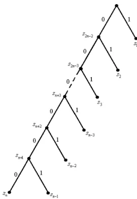
, (4) the source becomes anti-uniform.

After a binary Huffman encoding of the source with the distribution in (1) that fulfils (4), the graph in Fig. 1 is obtained.

Fig. 1. The graph of binary Huffman encoding for the source _n with distribution in (1) The structure of codewords resulting from binary Huffman encoding is:

 0 0 1 1 2 2 1 1 2 1 1 01 001 ... 00...01 00...00 n n n n n n s v s v s v s v s v              _{ }

The length l of the codeword associated with the message _i s is the number of edges on the _i

path between the root and the node s in the Huffman tree. _i

, 1, 2,..., 1 i l i i n (5) 1 n n l l_ (6) The average codeword length is determined with

1 1 1 ( 1) n n n i i i n i i l p l ip n p    







  . (7)

In Fig. 1 s_{n i} ,i1, 2,...,n denote the intermediate nodes in the graph, also called parents. 2 The probability of a parent is obtained as the sum of the two sibling probabilities. Denoting by p_{n i}

the probabilities of intermediate nodes, we have

; 1, 2,..., 2 n n i k k n i p _ p i n   



  (8) For a sequence of messages si the source delivers a string of binary symbols from the code alphabet

0 1

{ 0, 1}

X  x  x  . As the probabilities of symbols in the binary string depend on the node from which they are generated, the set X, which is the output bitstream obtained as result of binary Huffman coding is a source with memory.

When a terminal node ,s i_i 1, 2,...,n is reached, the source _nwill deliver another message and the source with memory X will generate another string of binary symbols.

The graph attached to the source with memory X can be obtained from the Huffman encoding graph in Fig. 1, as follows:

a) We link the terminal nodes with the graph root;

b) The branches between succesive nodes have the probabilities equal to the ratio between the probability of the node in which the branch ends and the probability of the node from which it starts, excepting the branches linking the terminal nodes with graph root, whose probabilities are equal to unity;

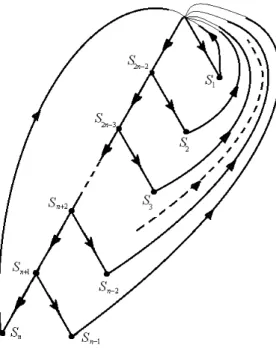
c) Each terminal node ,s i_i 1, 2,...,n, or intermediate ones s_{n i} ,i1, 2,...,n , (excepting the 2 root of the encoding graph) will represent the states S i_i, 1, 2,..., 2n , of the souce with memory 2 X. The set of these states is denoted by S { ,S S_{1 2},...,S_2n2} The graph of the source X is shown in Fig. 2.

Fig. 2 The graph of the source with memory X

The transition probabilities from the state Si, in the state Sj, that is, (p Sj|S , is equal to the i)

probability of the branch between the node Si and the node Sj. When the source enters the state Sj

from the state Si, it generates either the symbol x0 , or 0 x1 . Therefore, the probability of 1

delivering the symbol x_j,j0,1, from the state Si is the same as the probability to reach the state Sj,

starting from the state Si, that is:

1 1 1 ( | _i) ( | _i) , 1, 2,..., p x S  p S S  p i n (9) 0 2 2 2 ( | ) ( | ) , 1, 2,..., n i n i k k p x S p S _ S p i n   



 (10) 1 ( | ) ( | ) n i , 1, 2,..., 2 n i n i n i n k k n i p p x S p S S i n p          



(11) 1 0 1 ( | ) ( | ) , 1, 2,..., 2 n k k n i n i n i n i n k k n i p p x S p S S i n p           



 



(12)

Considering (9), (10), (11) and (12) as well as the graph in Fig. 2, the transition matrix between states is:

1 2 2 1 1 2 2 3 2 2 1 2 1 2 1 2 1 1 1 2 1 2 2 2 2 0 0 0 0 0 0 0 0 0 0 0 0 0 0 0 0 0 0 0 0 0 0 0 0 0 0 0 0 0 0 0 0 0 0 0 0 T n n n n n n n n k k n k k n k k n k n k n n n k k k n k n n k n k n n n k k k n k n n k k S S S S S S S S S p p p p p p p p p p p p p p p p                        





















                                  1 2 1 2 3 2 2 2 0 0 0 0 0 0 n n n n k k n n k k S S S S S p S p                                                                 





    (13)

where the entries of the matrix T are tij=p(Sj|Si).

Let ,_i i1, 2,..., 2n2, denote the stationary state probabilities of the source with memory. They can be determined by means of [22]

1 2 2 2 1 2 2 2 [ ,  ,..., _n ][ ,  ,..., _n ]T (14) 2 2 1 1 n i i    



(15) Considering (7) and (13), from (14) and (15) we obtain the state probabilities as:

, 1, 2,..., i i n p i n l    (16) 1 , 1, 2,..., 2 n n i k k n i n p i n l  _   



  (17) Generally, the entropy of the source with memory is computed by [23]

 

 

2 2 2 1 1 ( ) log n i j i j i i j H X  p x S p x S     

 

  (18) where _i are given in (16) and (17) and p x S

 

_j are given in (9), (10), (11) and (12). _i

Let c and ₀ c be the costs of storing or transmission of symbols “0” and “1”, respectively, ₁

resulted after the binary Huffman encoding of source _n. The average cost is determined by [9]



0 0 1 1



1 ( ) ( ) n i i C p n i c n i c  



 , (19) where n i and ₀( ) n i denote the number of 0’s and 1’s in the codeword ₁( ) c . _i

Considering the structure of codewords for AUH sources, (5) and (6), the average cost is



0 1



0 1 ( 1) ( 1) n i n i C p i c c n c p  



    (20)

3. Case studies for distributions leading to AUH sources

For all distributions we considered, we are interested to found out the condition imposed to the source parameter so that it is AUH, to derive the code entropy and the average cost.

3.1. AUH sources with geometric distribution

Let there be a discrete source characterized by the geometric distribution:

1 2 3 2 1 1 2 3 : 1 (1 ) (1 ) (1 ) n n n n s s s s p p p p p p p p p p p  _{ } _             , (21)

In this case the source is not complete, because

1 1 n n i i p p   



. (22) To form a complete source, we normalize the probabilities pi in (21), resulting the complete

source with distribution:

1 2 3 2 1 1 2 3 : 1 (1 ) (1 ) (1 ) 1 1 1 1 n norm n n n n n n n s s s s p p p p p p p p p p p p p p p      _{   }   _{   }   _{   }      (23)

For this source to become AUH, relation (4) is required to be fulfilled. Replacing the probabilities from (23) in (4), we have [18]:

5 1 0

2

p 

  (24) The average codeword length results by replacing the probabilities pi from (23) into (7).

1 1 1 1 ( 1) ( 1) (1 )(1 ) norm n n n n n l p n p n p p p      _      _   (25) Theorem

The entropy and the average cost of the source with memory resulted by binary encoding of the AUH source with Poisson distribution are determined by:

1

1 1 ( 1)

( ) log(1 ) log(1 ) log

(1 )(1 ) n n n n _norm n n np n p H X p p p p p p l         _     _     (26) 1 1 0 1 1 1 ( 1) (1 ) 1 1 n n n n _n np n p C p c pc p p         _   _  _  _ (27) Proof

The stationary state probabilities are obtained by replacing the probabilities pi from (23) into (16)

and (17), and considering (25):

1 1 1 (1 ) , 1, 2,..., (1 ) (1 ) , 1, 2,..., 2 (1 ) i i _{n norm} n n i i n i _{n norm} n p p i n p l p p i n p l            _  _   _   _{ }  _ (28)

The probabilities to deliver the symbol x₀  and 0 x₁ , from the states ,1 S i_i 1, 2,..., 2n , result 2 by replacing the probabilities pi from (23) into (9) – (12):

1 1 0 1 1 0 1 1 ( | ) , 1, 2,..., 1 (1 ) ( | ) , 1, 2,..., 1 1 ( | ) , 1, 2,..., 2 1 (1 ) ( | ) , 1, 2,..., 2 1 i n n i n n i i i n i i p p x S i n p p p p x S i n p p p x S i n p p p p x S i n p          _  _     _     _        _   _{ }  _ (29)

Substituting (23) into (20), the relation (27) results.

When the number of messages, n, of the source _nincreases, at limit, when n  ,we have 1 1 l p    (30) ( ) log (1 ) log(1 )       H X p p p p (31) 0 1 1 p C c c p     (32)

3.2. AUH sources with quasi-geometric distribution

Let there be a discrete source characterized by the quasi-geometric distribution:

1 2 3 1 1 2 3 2 1 2 2 : 1 2 2 2 2 n n n n n n n s s s s s p p p p p p p p p p           _{     }        , (33)

Following similar procedures as in the previous case, we get: - The range for the source parameter for the source to be AUH

2 0

3

p

  . (34) - The average codeword length

2 3 2 1 1 2 n n _n l p      (35) - The entropy of the source with memory X

1 1 1 1 (1 ) log(1 ) [1 ( 1) ] log ( ) 1 ( 1) ( 1) n n n n n n n p p np n p p p H X p n p n p                  (36)

- The average cost of the source with memory X

1 2 1 0 2 (2 1) (2 ) 2 n n n n pc p c C        (37) When n , we have 1 ( ) [(1 ) log(1 ) log 2 ] 1 2 H X p p p p p p    _     (38)

1 0

2

C  pc c (39)

In the special case, when 1

2 

p , the source  becomes dyadic one. In this case X becomes _n memoryless and then:

1 ( | ) , 0,1; 1, 2,..., 2 2 2 j i p x S  j i n , (40) 2 1 2 2 dn _n l   _ (41) ( ) 1 dn H X  (42) 1 1 0 1 (2 1)( ) 2 n dn n C C C      (43) Imposing n  in (41) and (43), we have

2 d l   (44) 0 1 d C    (45) c c

3.3. AUH sources with Fibonacci distribution

Let there be a discrete and finite AUH source characterized by the Fibonacci distribution

1 2 2 1 1 2 2 1 1 1 2 2 1 1 1 1 1 1 : n n n n n n n n n n n n n n s s s s s f f f f f p p p p p f f f f f  _{ }               _{    }        (46)

where f is the n_n th Fibonacci number defined as

1 2 1 2 1 , 3         _{ } n n n f f f f f n (47)

The source _n is also AUH, because relation (4) is fulfilled. - The average codeword length

3 1 3 n n n f l f     (48)

- The entropy of the source with memory X 1 1 1 1 3 3 1 ( ) log log 3 3          



n n n n i i i n n f H X f f f f f (49)

- The average cost of the source with memory X

1 1 2 0 1 1 1 n n n n n f f f C c c f f        (50)

3.4. AUH sources with exponential distribution

The density probability function of exponential distribution is

, 0 ( , ) 0, 0    _{ }     x e if x f x if x (51)

We define the cumulative density function

( ) 1 i

F i e , (52)

and the probabilities

( 1)

( ) ( 1)   (1 )

    i 

i

p F i F i e e . (53)

Let us consider the source _nwith exponential distribution

1 2 1 ( 2) ( 1) 1 2 1 1 : 1 (1 ) (1 ) (1 ) n n n n n n n s s s s p e  p e  e  p e  e  p e  e                  _{       }      (54)

- The range for the source parameter for the source to be AUH [8]

5 1 ln

2

 _  _

  (55) - The average codeword length

( 1) ( 1) 1 1 ( 1) ( 1) (1 )(1 ) norm n n n n n l e n e n e e e                _      _   (56)

- The entropy of the source with memory X

( 1)

1 1 ( 1)

( ) log(1 ) log(1 ) log

(1 )(1 ) n n n n _norm n n ne n e H X e e e e e e l                        _     _     (57)

- The average cost of the source with memory X ( 1) ( 1) 0 1 1 1 ( 1) (1 ) 1 1 n n n n _n ne n e C e C e C e e                     _   _  _  _ (58) When n , we have log ( ) (1 ) log(1 ) 1 e e H X e e e                 _   _    (59) 0 1 1 e C c c e      _   (60) 0 1 ( 1) (1 ) 1 k k l k e e e        _      



. (61)

3.5 AUH sources with Poisson distribution

Let there be a discrete source with infinite alphabet, characterized by Poisson distribution: 0 1 2 2 0 1 2 : 1! 2! ! n n n n s s s s p e p e p e p e n      _{      }      _{   }        , (62)

- The range of the parameter for the source to be AUH [18] 1

 (63) - The average codeword length

1

l  . (64) 

The entropy of the source with memory X

1

1

( ) log log log( !)

1 ! n n H X e e n n              _   _  



 (65)

The average cost of the source with memory X

0 1

3.6. AUH sources with negative binomial distribution

Let there be a discrete source with infinite alphabet, characterized by the negative binomial distribution: 0 1 2 1 1 1 2 1 0 1 1 2 1 1 : n n r r r r r r r r n r r r n r n s s s s p C p p C p q p C p q p C p q  _{   }        _{   }      , (67) where q=1-p.

- The average codeword length

1 1 0 ( 1) r r n r n n rq p l n C p q p    _{ }   



  . (68) The entropy of the source with memory X

1 1

1 1

1

( ) log log r r klog r

r n r n n p qr H X r p q p C q C rq p p              _   _  



 (69)

The average cost of the source with memory X

0 1 qr C c c p    (70) 7. Conclusions

In this paper we have considered the class of AUH sources with finite and infinite alphabets. Performing a binary Huffman encoding of these sources, we show that sources with memory result. For these sources we build the encoding graph and the graph of the source with memory X. The graph of the source with memory is obtained from the encoding graph by linking the terminal nodes with the graph root. The states of the source with memory correspond to the terminal or intermediate nodes in the encoding graph, excepting the root. We determined in the general case the state probabilities of the source with memory, as well as the transition probabilities between states. The entropy of this source with memory is computed. We assumed the costs c0 and c1 for the

symbols “0” and “1”, respectively, and compute the average cost for these Huffman codes. Obviously, the Huffman encoding procedure assures minimum average length, but the average cost is not minimum. It can be easily verified that if the costs of symbols “0” and “1” are equal to unity,

the average cost becomes equal to the average length. We applied the results for several AUH sources with geometric, quasi-geometric, Fibonacci, exponential, Poisson and negative binomial distributions. We have also analyzed the limit cases, when the source alphabet increases unlimited, that is, n  .

References

[1] R. Huffman, “A method for the construction of minimum – redundancy codes,” Proc. IRE, vol. 40, pp. 1098 – 1101, 1952.

[2] T. Linder, V. Tarokh, K. Seeger, “Existence of optimal prefix codes for infinite source alphabets,”

IEEE Trans. Inf. Theory; vol. 43, No. 6, pp. 2026-2028, Nov. 1997

[3] R. M. Capocelli, A. De Santis, “A note on D-ary Huffman codes,” IEEE Trans. Inf. Theory vol. 37, No.1, pp. 174-191, Jan. 1991.

[4] R. Gallager, “Variations by a theme of Huffman,” IEEE Trans. Inf. Theory vol. 24, No. 6, pp. 668-74, Nov. 1978.

[5] O. Johnsen, “On the redundancy of binary Huffman codes,” IEEE Trans. Inf. Theory, vol. 26, No. 2, pp. 220-222, March, 1980.

[6] M. Khorsavifard, M. Esmaeili, H. Saidi, T.A. Gulliver, “A tree based algorithm for generating all possible binary compact codes with N codewords,” IEICE Trans. Fundam. Electron. Commun.

Computer Sci., vol. E86-A, No. 10, pp. 2510-2516, Oct. 2003.

[7] M. Esmaeili, A. Kakhbod, “On antiuniform and partially antiuniform sources,” Proc. IEEE ICC, pp. 1611 – 1615 June 2006

[8] S. Mohajer, A. Kakhbod, “Anti – uniform Huffman codes,” IET Commun., vol.5, pp. 1213 – 1219 2011.

[9] S. Mohajer, A Kakhbod, “Tight bounds on the AUH codes,” Information Sciences and Sysyems, 2008. CISS 2008. 42nd Annual Conference on, pp. 1010 – 1014, 19 – 21 March

[10] S. Mohajer, P. Pakzad, A. Kakhbod, “Tight bounds on the redundancy of Huffman codes,” Proc.

IEEE ITW, , pp. 131 – 135, March, 2006.

[11] O. Johnsen, “On the redundancy of binary Huffman codes,” IEEE Trans. Inf. Theory. vol. 26, pp.220-222, 1980.

[12] P. Bradford, M Golin, L. L. Larmore and W. Rytter, “Optimal prefix free codes for unequal letter costs and dynamic programming with the Monge property,” J. Algorithms, vol. 42, pp. 277 – 303, 2002.

[13] E. N. Gilbert, “Coding with digits of unequal costs,” Trans. Inf. Theory. vol. 41, pp. 596-600, 1995. [14] M. Golin, G. Rote, “A dynamic programming algorithm for constructing optimal prefix-free codes

for unequal costs,” IEEE Trans. IT 44(5):1770-1781, 1998.

[15] T. Berger, R. Yeung, “Optimum 1-ended binary prefix codes,” Trans. Inf. Theory. vol.36 No.6, pp. 1434-1441, Nov. 1990.

[16] A. De Santis, R. M. Capocelli, G. Persiano “Binary prefix codes ending in a 1 Trans. Inf. Theory. vol. 40, pp. 1296-1302, July 1994.

[17] E. Korach, S. Dolov and D. Yukelson, “The sound of silence: Guessing games for saving energy in mobile environment,” In Proc. Of the Eighteenth Annual Joint Conference of IEEE Computer and Communications Societies (IEEE INFOCOM’99), pp. 768-775, 1999.

[18] M. Esmaeili, A.Kakhbod, “On information theory parameters of infinite anti-uniform sources,” IET

Commun., vol.1, pp. 1039 – 1041, 2007.

[19] P. Humblet, “Optimal source coding for a class of integer alphabets,” IEEE Trans. Inf. Theory, vol 24, No.1, pp. 110 – 112, 1978.

[20] R. Gallager, D. Van Voorhis, “Optimal source coding for geometrically distributed integer alphabets,” IEEE Trans. Inf. Theory, vol. 21, No. 2, pp. 228 – 230, 1975.

[21] M. Esmaeili, A. Gulliver and A. Kakhbod, “The Golden Mean, Fibonacci Matrices and Partial Weakly Super-Increasing Sources,” Chaos, Solitions and Fractals, Vol. 42, No. 1, pp. 435 – 440, 2009.

[22] J. G. Kemeny, T. L. Snell, Finite Markov Chains, Princeton, NJ: Van Nostrand, 1960.

[23] T. M. Cover, J. A. Thomas, Elements of Information Theory. John Wiley and Sons, Inc. New York, 1991.