HAL Id: hal-02529409
https://hal.archives-ouvertes.fr/hal-02529409
Submitted on 2 Apr 2020
HAL is a multi-disciplinary open access
archive for the deposit and dissemination of
sci-entific research documents, whether they are
pub-lished or not. The documents may come from
teaching and research institutions in France or
abroad, or from public or private research centers.
L’archive ouverte pluridisciplinaire HAL, est
destinée au dépôt et à la diffusion de documents
scientifiques de niveau recherche, publiés ou non,
émanant des établissements d’enseignement et de
recherche français ou étrangers, des laboratoires
publics ou privés.
3D Analytical Modelling of Sink Heat Distribution for
Fast Optimisation of Power Converters
Anne Castelan, Bernardo Cougo, Sébastien Dutour, Thierry Meynard
To cite this version:
Anne Castelan, Bernardo Cougo, Sébastien Dutour, Thierry Meynard. 3D Analytical Modelling of
Sink Heat Distribution for Fast Optimisation of Power Converters. Electricmacs 2017, Jul 2017,
Toulouse, France. pp.296-307. �hal-02529409�
Any correspondence concerning this service should be sent
to the repository administrator:
tech-oatao@listes-diff.inp-toulouse.fr
To cite this version:
Castelan, Anne and Cougo, Bernardo and Dutour, Sébastien and
Meynard, Thierry 3D Analytical Modelling of Sink Heat Distribution for
Fast Optimisation of Power Converters. (2019) In: Electricmacs 2017,
4 July 2017 - 6 July 2017 (Toulouse, France).
ELECTRIMACS 2017, 4th -6th July 2017, Toulouse, France
3D
A
NALYTICAL
M
ODELLING OF
H
EAT
S
INK
H
EAT
D
ISTRIBUTION
FOR
F
AST
O
PTIMISATION OF
P
OWER
C
ONVERTERS
A. Castelan
1,2,3, B. Cougo
1, S. Dutour
3, T. Meynard
21. IRT Saint-Exupéry, 118, route de Narbonne - CS 44248, 31432 Toulouse cedex 4, France 2. LAPLACE, INP-ENSEEIHT, 2 rue Charles Camichel - BP 7122, 31071 Toulouse cedex 7, France 3. LAPLACE, Université Paul Sabatier - Bat3R3, 118 route de Narbonne, 31062 Toulouse cedex 9, France
E-mail: anne.castelan@irt-saintexupery.com
Abstract - With the development of embedded systems, it is crucial to reduce
weight of equipments. In power converter, heat sink is a heavy part that often can be reduced in volume and weight. There are several models and methods to calculate a heat sink thermal resistance. However the more precise these methods are, the more time consuming they are and thus they can be hardly integrated in a weight optimization routine. Using analytical models to calculate heat sink thermal resistance is a good compromise between execution time and precision of results. They are usually one-dimensional models which are simple but do not take into account heat spreading effects, which is important when power electronic heat sources are small compared to their heat sink. This paper describes a three-dimensional analytical model of forced convection plate fin heat sink, which will be compared with numerical simulation. A maximum difference of 2.5% has been observed between models. This analytical model will be used in an optimization routine to reduce the weight of an existing heat sink in order to show that fast and precise optimization of cooling system is possible with analytical models.
Keywords – Heat Sink, 3D FEM Simulation, Analytical Modelling, Power
Converter, Optimization.
1. INTRODUCTION
Real development of more electrical aircraft is only possible if high level of equipment integration is achieved, i.e. if one can reduce at most the system’s mass and increase power density. One of the most important equipments that must be optimized is a static power converter, which can be found in many applications inside an aircraft.
Designing a power converter always implies on finding the best trade-off between cost, mass, efficiency and reliability applied to the different elements such as capacitors, inductors, switches, cooling system (heat sinks), control boards and etc. Most of the times, the heat sink, which is one of the heaviest elements, is only evaluated at the end of the design process and is often oversized.
Heat sinks are full metal components, usually made of aluminium and sometimes of copper and other metals. Heat is dissipated by natural or forced convection. Thus, heat sink is a heavy element, which significantly contributes to the converter weight. For that reason increasing power density of a power converter implies on reducing at maximum the heat sink weight.
Moreover, since reliability is a major aspect in any aircraft application, liquid cooling heat sink should be avoided. The use of pumps and fluid circulation circuits requires regular maintenance and decreases system reliability. For that reason, it is essential to use fin heat sinks in natural or forced convection. Weight optimization of fin heat sinks can be only achieved by the use of adapted models, which are precise enough to design a valid device but fast enough to be executed in a reasonable time. Calculation of heat sink thermal resistances and temperatures is possible either by very precise 3D Finite Element Method (FEM) simulations or by analytical models. FEM simulations are very time consuming and are hardly integrated in optimization routines. On the other hand, analytical modelling is usually fast but inaccurate. Our goal is to then develop a heat sink analytical model, which is fast enough to take part of a power converter optimization routine, and at the same time fairly precise (maximum 5% difference between analytical calculation and FEM simulation).
Modelling shown in this paper concerns forced convection heat sinks with plate fins which is one of the most robust, cheap and thus common types of cooling systems.
The analytical model developed to describe a plate fin heat sink will be introduced in this paper. The goal of this model is to give the mean heat source(s) temperature(s). A state of art of an existing model will be first presented before we develop the model used in our optimization routines. After that, a comparison between FEM and the developed analytical model will be shown in order to confirm that it is precise enough to be used for fast design. Finally, this model will be integrated in an optimization routine. A thermal system design has been made. An example of heat sink design for a power converter used in aircraft applications will be shown. This example illustrates how fast the developed optimization routines are and the importance of taking into account heat spreading in the baseplate of the heatsink.
2. STATE
OF
ART
OF
EXISTING
MODELS
There are different studies for heat sink weight reduction, however developed models are either very simple (proportional relation between weight and thermal resistance, often used for predesigning components), or very complex (using FEM software).
Analytical models of different forms used to describe heat sink with plate fins, in forced or natural convection, are found in literature. These models are most of the time resistive models, and are generally based on one-dimensional approximations [1, 2, 3]. The main advantage of these models is that they are easy to employ since they are similar to electrical models.
There are also two or three-dimensional models, coming from direct resolution of heat transfer equations and that are then more precise models [4, 5, 6, 7, 8, 9, 10]. The main advantage of these 2D/3D models is that they consider more realistic propagation effects of the heat produced by the heat source (usually power components). Power components are usually smaller than the heat sink baseplate and like so there is a real spreading effect of the heat in this baseplate. This spreading phenomenon is not easily and precisely described with resistive models based on one-dimensional approximations.
For that reason, the approach proposed in this work combines the general 3D description of heat spreading as shown in [10] and a fin model to obtain an analytical description of the whole thermal component. Thus, many different configurations, size and position of heat sources and heat sink can be considered.
3. HEAT
SINK
MODEL
Heat sink and fan models are based on geometrical parameters shown in Fig.1. These parameters are the fin height HFIN, the baseplate thickness HBP, the length L and width W of the heat sink, the space between fins b, corresponding to the channel where air is pulsed by the fan, the fin thickness TFIN and the number of fins nFIN.
Fig.1 : Geometrical parameters of extruded heat sink and fan.
Heat sink design procedure is schematically shown in Fig. 2. Inputs of this procedure are: number, size, location and power of heat sources; heat sink geometry (number of fins, geometrical dimensions) heat sink material and fan characteristics. Outputs (results) are the values of the average temperature of each heat source, as well as the weight value of the cooling system (heat sink + fan). Note that a thermal resistance RTH of the cooling system can be calculated in the case of only one heat source connected to the heat sink.
Different constraints can be added to the design procedure such as the maximum and minimum values of geometrical parameters or the maximum temperature of heat sources.
Blocs 1 to 3 of Fig. 2 concern the choice of heat sink geometrical parameters and fan, the determination of fan operation point (based on the calculation of static pressure drop of the heat sink) and the calculation of the equivalent fin thermal resistance which is determined based on the aeraulic model applied to the fins. This model is established by a Nusselt number correlation. Details on this calculation are already given in [11] and will not be presented here.
Instead, this paper explains in details Bloc 4 and Bloc 5. In these blocs, thermal resistance values calculated for each fin (RTH_FIN) is used to calculate an equivalent heat transfer coefficient (qEQ) which will be applied to the entire bottom surface of the heat sink baseplate. In this way, heat spreading can be calculated in Bloc 5 with model of [10], which gives a 3D model of the baseplate. This procedure is schematically shown in Fig. 2.
ELECTRIMACS 2017, 4th -6th July 2017, Toulouse, France
Fig. 2: Design procedure to optimize the weight of cooling system composed of heat sink and fan.
Fig. 3: Equivalence between fin thermal resistance (RTH_FINS) and heat exchange coefficient (qEQ) in
order to calculate heat spreading in heat sink baseplates.
3.1. BASEPLATE MODEL
This equivalent heat transfer coefficient qEQ between the lower surface of the base plate SBASEPLATE and the ambient is determined from the thermal resistance of fins as follows: BASEPLATE FINS TH EQ
S
R
q
_1
(1)where RTH_FINS sums up all the thermal transfer existing in the fins, i.e. conduction along the fins and convective transfer with the ambient air:
L b h N R N R AMB FINS FIN TH FINS FINS TH 1 1 _ _ (2)
Where hAMB is the convective coefficient applied to fin surface and given by the aeraulic model and the Nusselt correlation. RTH_FIN is the thermal resistance of one single fin, given by (3). In this last equation,
SFIN is the product TFIN∙L, λFIN is the fin conductivity
and α is given by (4). ) tanh( 1 _ FIN FIN FIN FIN TH H S R (3) FIN FIN FIN AMB S L T h 2 ( ) (4)
Then, solving the heat diffusion in the base plate [10], it is possible to determine the mean temperature of the heat source, whatever its position is, with the relation:
) 5 . 0 sin( ) cos( ) 5 . 0 sin( ) cos( 4 ) 5 . 0 sin( ) cos( 2 ) 5 . 0 sin( ) cos( 2 1 1 , 1 1 1 c X d c d Y A d d Y A c c X A T T m c m m n m n n c n n m n n n c n n m m m c m m D AMB SOURCE
(5)
is the mean temperature rise of the heat source when compared to ambient temperature and) 1 ( 1 EQ BP D q H L W Q
(6)Fourier coefficients Am, An, Amn are given in [10] and depend on the source dimension, the power evacuated, the source position on the baseplate, the dimensions of the baseplate and the heat transfer coefficient applied on the bottom of the baseplate. Complete details of these expressions are shown in [10]. λm, δn, βmn, are the eigenvalues of each part of the solution. Parameters c and d correspond to the width and the length of the heat source; XC and YC are the coordinates of the heat source center point referred to a baseplate corner. Q is the power dissipated by the source, a and b are the width and the length of the baseplate, HBP is the baseplate thickness, λ is the baseplate conductivity, and qEQ is the heat transfer coefficient of (1).
As shown in [10], in a system with Ns heat sources, superposition can be applied to calculate the mean temperature rise of each heat source. For that, one must take into account the influence of all heat sources in order to calculate the mean temperature rise in one heat source. This can be calculated, for a certain heat source “j” as:
Ns i i AMB j SOURCE T T 1 (7) Where TSOURCEj is the mean temperature of source “j”, TAMB the temperature of the air around the heat sink, and i the mean temperature rise contributionof all sources, calculated at the coordinates of the source “j”. It means that i has the same analytical
expression as (5) for a single source, however Fourier coefficients are evaluated at the source “i“, but the temperature expression is evaluated at the source “j” coordinates and dimensions. The complete details of these expressions are also described in [10].
4. NUMERICAL
COMPARISON
Once this analytical model is established, it is necessary to quantify the difference of results using this analytical model and a precise 3D numerical simulation with finite element methods (FEM). This numerical comparison of the analytical model is performed using COMSOL software.
A complete heat sink (baseplate and fins) has been realized as shown in Fig. 4 for a given dimension of heat sink and heat source. Same dimensions and heat source have been used in both models (analytical and FEM simulation).
Heat sink has 17 fins of 6.1mm thickness and 40mm height. Baseplate has dimensions: thickness
HBP=0.009m, length L=0.1m and width W=0.2m. The square heat source is centered, and has initially width and length (respectively c and d) of 0.02m and it dissipates 100W. Width and length of the heat source will vary during the study. The convective heat transfer applied uniformly on fins is 50 W/m²K in order to simulate a wind speed of approximately 1m/s. The choice of using this uniform convective heat transfer coefficient is related to the fin thermal model we used since the aeraulic model gives an average coefficient along the fins.
Fig. 4 : Example of simulation result of heat sink with plate fins in forced convection used to compare
with the developed analytical model. For different ratio of heat source dimensions and baseplate dimensions, a maximum difference of 2.5% has been observed in the calculation of the heat source mean temperature rise between analytical and numerical models. This difference is shown in Fig. 5 where the dimensions of the heat source is changed so its surface is varied from 5% to 50% of the baseplate surface. As it can be seen in this figure, when the heat source size increases, this difference decreases. This increase of surface reduces the spreading effect and brings the configuration close to a one-dimensional conduction case in the base plate.
When several sources are simulated on the baseplate, low difference between the two models can also be observed.
The use of analytical model gives results almost as precise as finite element method model, on simple configurations. However, analytical model execution is very fast compared to numerical model. In this specific case, the resolution of a numerical model took about 15 minutes in a dual-core Intel Xeon, 3.2GHz having 64GB of RAM memory; and about 5.5ms for the analytical calculation in a Personal Computer having an Intel Core i7, 1.8GHz and 8GB of RAM memory.
Fig. 5 : Difference between the heat source mean temperature rise evaluation using the proposed analytical model and a 3D FEM simulation for
different heat sources dimensions.
5. O
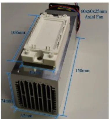
PTIMIZATIONUsing the proposed analytical model in a optimization routine is certainly interesting because this model has a very fast calculation and also considers heat spreading in the baseplate of a heat sink, which is not the case of models in [4,5]. The baseplate is, in several heat sink designs, the heaviest part of the heat sink. Thus, having a precise model of heat spreading in this baseplate will help reducing the weight and then improving the integration of the heat sink into the power converter. In order to illustrate the influence of the baseplate in the heat sink thermal resistance and also the use of the proposed models in the optimization of a heat sink, an example is given below. A three-phase power inverter for aircraft applications using a SiC module (reference CCS050M12CM2, from manufacturer CREE) of nominal power of 15kW is used as reference. Losses at this power module are dissipated in a high performance forced air-cooling system of reference LA6 150, from manufacturer FischerElektronik. This cooling system has a thermal resistance of 0.175K/W at maximum fan power. Note that this thermal resistance value is given for a heat source of the same size as the heat sink baseplate. Fan weight is 0.066kg and the aluminium heat sink weight is 0.830kg. Dimensions of heat sink and heat source (power module) are given in Fig. 6.
ELECTRIMACS 2017, 4th -6th July 2017, Toulouse, France
In a first example, we show the influence of the baseplate in the total thermal resistance. We consider a heat sink with 30 fins of 26.6mm height, a baseplate of 50.6mm width, 150mm length and a baseplate thickness varying from 3 to 20mm. The heat source is the power module, having dimensions of 47mm width and 108mm long. Calculation of thermal resistance of the heat sink using the proposed heat spreading model (3D model) and using a 1D model is shown in Fig. 7 for the baseplate thickness variation. It can be seen that, when baseplate thickness increases, heat sink thermal resistance decreases up to a minimum point and then it increases using the 3D model while it always increases using the 1D model. The difference between the maximum and minimum thermal resistance using the 3D is not that high given that the surface of the heat source is close to that of the baseplate. For the same reason, the difference between the 3D and 1D models is not so high (about 8% at thickness of 3mm). Obviously, this different could be much higher for heat sources with smaller surface.
Fig. 6: Heat sink, fan and power module used as reference in the example of heat sink optimization.
Fig. 7: Variation of the global thermal resistance of a heat sink with the baseplate thickness using 1D and 3D models. Because the heat source surface is
close to that of the hat sink baseplate, 3D effect is not so high.
In the second example, the analytical model is coded in MATLAB using an optimization routine based on parametrical variation of 6 parameters. The fan characteristic is the same as the one for the first
example. Since the analytical model is very fast to compute, many points for each parameter can be calculated and no optimization technique is needed. The heat sink of Fig. 6 is used as a reference design for comparison, having a thermal resistance of 0.175K/W. Given the geometrical and mechanical constraints for the insertion of this heat sink in the real SiC converter, parameters were varied as follows: Heat sink length L from 108 to 150mm (5 points), width W from 47 to 62mm (5 points), base plate thickness HBP from 3 to 20mm (9 points), fin height HFIN from 10 to 80mm (9 points), number of fins nFIN from 10 to 40 and a k=nFIN·TFIN/W factor from 0.01 to 0.09 (total of 11 points, this parameters gives an idea of the fin thickness TFIN). The heat source is the same SiC module having 47mm width and 108mm length.
After 40 minutes of calculation of 690525 options, the routine found the minimum thermal resistance of 0.1535K/W for a weight of 0.984kg (0.918kg the aluminum heat sink and 0.066kg the fan). Note that this optimal heat sink has about 12% less thermal resistance than reference one but it is slightly heavier.
Fig. 8: Thermal resistance for different number of fins and fin thickness (expressed by the k factor). In
this example, the minimum thermal resistance is marked with a circle and it is the same as reference one. However, the mass of this optimal heat sink is 0.403kg which is 55% lower than the reference one. Searching in all the results, one can find the minimal system weight for the same thermal resistance as the reference. It results in a minimum weight of 0.403kg for a thermal resistance of 0.175K/W. This optimal heat sink design is slightly lower than half the weight of the reference heat sink. This optimization has 6 variables and all the results cannot be shown in one graph. However, in order to illustrate, 4 parameters were fixed at the optimal point (L=119mm, W=62mm, HBP=3mm and HFIN=54mm) and variables nFIN and k were varied. Curves related to the calculation of thermal resistance are shown in Fig. 8. Note that it achieves the minimum value of 0.175K/W at nFIN=26 and k=0.34. Also note that, for each different k (also each different fin thickness), there is an optimal number of fins which minimizes
the thermal resistance. Obviously, the lower the number of fins, the lower the weight. These results are summarized in Table 1.
Rth (K/W) Weight (kg)
Optimization of Rth 0.1535 0.984
Optimization of weight 0.175 0.403
Heat sink reference design 0.175 0.896 Table 1: Summary of results obtained after optimization of heat sink thermal resistance and weight.
6. C
ONCLUSIONHeat sink optimization is one of the most important aspects to take into account when reducing weight of power converters. Accurate 3D FEM simulations can be used but they are so time consuming that they are hardly included in optimzation routines. Analytical models are fast but usually not enough accurate. For that reason, we developed an analytical modeling to calculate heat source mean temperature which is accurate and take into account heat spreading in the heat sink baseplate. This is particularly important when heat sources have a surface much smaller than that of the baseplate. The developed model can also be used in problems with more than one heat source. In this manner, it calculates the average temperature of each heat source.
This analytical model was compared to precise 3D FEM simulation. Difference of no more than 2.5% was observed between results of analytical model and 3D FEM simulation. However, we observed an extreme gain on time using this analytical model. For a given heat sink geometry, calculation of thermal resistance took about 5.5ms using analytical model and about 15 minutes (about 160000 times slower) using a 3D FEM simulation.
The developed analytical model was used in a optimization routine in order to reduce the size of an existing performant heatsink+fan system. Optimization results show a reduction of about 12% on the thermal resistance if the objective is to reduce this value, or a reduction of 55% of the cooling system weight if the thermal resistance value of the existing heatsink+fan system is used as reference for the optimization routine.
R
EFERENCES[1] R. E. Simons, Simple formula estimating thermal spread resistance, https://www.electronics-cooling.
com/2004/05/simple-formulas-for-estimating-therm al-spreading-resistance/, accessed in January 2017 [2]S. Song, S. Lee, V. Au, Closed form equation for thermal constriction spreading resistance with variable boundary condition, http://www.aavid.com /sites/default/files/technical/papers/closed-form-equation.pdf, accessed in January 2017.
[3]S. Song, S. Lee, V. Au, K. Moran, Constriction spreading resistance model for electronics packaging, http://www.aavid.com/sites/default/files/ technical/papers/constriction-resistance-electronics packaging.pdf , accessed in January 2017.
[4] U. Drofenik, A. Stupar, J. W. Kolar, Analysis of Theoretical Limits of Forced-Air Cooling Using Advanced Composite Materials with High Thermal Conductivity. IEEE Transactions on Components,
Packaging, and Manufacturing Technology, Vol. 1,
No. 4, pp. 528-535, April 2011.
[5] C. Gammeter, F. Krismer, J. W. Kolar, Weight Optimization of a Cooling System Composed of Fan and Extruded Fin Heat Sink. IEEE Energy
Conversion Congress and Exposition (ECCE USA 2013), Denver, Colorado, USA,September 15-19,
2013.
[6] M. M. Yovanovich, Y. S. Muzychka, J. R. Culham, Spreading resistance of isoflux rectangles and strips on compound flux channels. Journal of
thermophysics and heat transfer, vol. 13, n o. 4,
October-December 1999.
[7] M. M. Yovanovich, J. R. Culham and P. Teertstra, Analytical modeling of spreading resistance in flux tubes, half spaces, and compound disks. IEEE Transactions on Components, Packaging, and Manufacturing Technology: Part A,
vol. 21, no. 1, pp. 168-176, Mar 1998.
[8]D. Guan, M. Marz, J. Liang, Analytical Solution of Thermal Spreading Resistance in Power Electronics. IEEE Transactions on Components,
Packaging and Manufacturing Technology, 2(2),
278-285, 2012.
[9] M. J. M Krane, Constriction resistance in rectangular bodies. Journal of Electronic Packaging, 113(4), 392-396, 1991.
[10] M. M. Yovanovich, Y. S. Muzychka, J. R. Culham, Thermal spreading resistance of eccentric heat sources on rectangular flux channels. Journal of
Electronic packaging 125.2 :178-185, 2003.
[11] A. Castelan, B. Cougo, J. Brandelero, D. Flumian, T. Meynard, Optimization of forced-air cooling system for accurate design of power converters. IEEE 24th International Symposium on