Distributed approximation of open-channel flow routing accounting for backwater effects

(1)

HAL Id: hal-00682721

https://hal.archives-ouvertes.fr/hal-00682721

Submitted on 26 Mar 2012

HAL is a multi-disciplinary open access archive for the deposit and dissemination of sci-entific research documents, whether they are pub-lished or not. The documents may come from

L’archive ouverte pluridisciplinaire HAL, est destinée au dépôt et à la diffusion de documents scientifiques de niveau recherche, publiés ou non, émanant des établissements d’enseignement et de

Distributed approximation of open-channel flow routing

accounting for backwater effects

Simon Munier, Xavier Litrico, Gilles Belaud, P.-O. Malaterre

To cite this version:

Simon Munier, Xavier Litrico, Gilles Belaud, P.-O. Malaterre. Distributed approximation of open-channel flow routing accounting for backwater effects. Advances in Water Resources, Elsevier, 2008, 31 (12), pp.1590-1602. �10.1016/j.advwatres.2008.07.007�. �hal-00682721�

(2)

Distributed approximation of open-channel

ﬂow routing accounting for backwater eﬀects

Simon Munier

a

Xavier Litrico

a

Gilles Belaud

b

Pierre-Olivier Malaterre

a

a_{Cemagref, UMR G-EAU, 361 rue J.F. Breton, B.P. 5095, 34196 Montpellier}

Cedex 5, France

b_{IRD, UMR G-EAU, Maison des Sciences de l’Eau, 300 Avenue Emile Jeanbrau,}

34095 Montpellier Cedex 5, France

Abstract

In this article, we propose a new model, called LBLR for Linear Backwater Lag-and-Route, which approximates the Saint-Venant equations linearized around a non-uniform flow in a finite channel (with a downstream boundary condition). A classical frequency approach is used to build the distributed Saint-Venant transfer function providing the discharge at any point in the channel in the Laplace domain with respect to the upstream discharge. The moment matching method is used to match a second-order-with-delay model on the theoretical distributed Saint-Venant transfer function. Model parameters are then expressed analytically as functions of the pool characteristics. The proposed model efficiently accounts for the effects of downstream boundary condition on the channel dynamics.

Key words: Open-channel ﬂow routing, Saint-Venant equations, frequency

response, Laplace transform

1 Introduction

Water resources are renewable but in limited supply. In a context of multi-ple needs, such as irrigation or domestic water supply, this resource has to

Email addresses: [email protected] (Simon Munier),

[email protected] (Xavier Litrico), [email protected] (Gilles Belaud), [email protected] (Pierre-Olivier Malaterre).

(3)

be collected, shared and then distributed using water transport systems, such as rivers and/or canals. Water managers control flows in such open-channels using hydraulic structures (dams, weirs, gates). The water distribution effi-ciency can be greatly improved by operating these structures using automatic tools. This requires models that are able to represent open-channel flow rout-ing with a desired accuracy. Nowadays, many systems are controlled usrout-ing linear controllers based on linear models since many methodologies and tools are well-known and validated for such systems. Linear approaches have also advantages in terms of simplicity, rapidity and robustness ([11,13,17]). Sev-eral authors used numerical schemes to obtain such linear models from the Saint-Venant equations ([1,10,21]). But they are usually high order models. Alternative approaches could be preferred to obtain lower order models with coefficients expressed analytically. This justifies the interest in improving such flow routing models.

Modeling of flow routing along a river stretch or a canal pool has been the subject of numerous articles since the 1950’s. A comprehensive review of ap-proximate flow routing methods has been presented in [28]. Different linear models have been developed for flow routing simulation purposes (e.g. [8,26]). Most of them are based on analysis of the linearized Saint-Venant equations around a reference flow. To greatly simplify the equations, the downstream boundary condition is usually neglected by considering a semi-infinite chan-nel (see e.g. [8]), leading to a uniform reference flow. However, a downstream boundary condition imposed by a hydraulic structure, such as a weir, has two different effects on the flow: it modifies the water depth, causing a backwater curve, and it enforces a local coupling, called feedback, between the discharge and water depth. But, even in a linear framework (i.e. for small variations), neglecting these two effects sometimes leads to large under- or over-estimation of some parameters such as the response time, peak time or the level of attenu-ation. The effects induced on the flow dynamics by the downstream boundary condition have been analyzed based on numerical simulations in [25]. Some analysis of the backwater effects has also been brought in [7] and [27], and has underlined the fact that the downstream boundary condition can sometimes provide significant modifications of the flow dynamics.

In this article, a new three-parameter model, called LBLR for Linear Backwa-ter Lag and Route, is derived and accounts for the effects of the downstream boundary condition. It takes the feedback and the backwater effects into ac-count separately, and provides the discharge at any point in the channel with respect to the discharge at the upstream end. The three parameters are ex-pressed analytically depending on the pool characteristics (length, geometry, roughness, reference flow), which provides a quick and accurate calculation of these parameters.

(4)

Saint-Venant equations, which generates transfer functions in the Laplace do-main. In this framework, the introduction of a downstream boundary condi-tion is equivalent to a local feedback between the discharge and the water level deviations. A moment matching method is then used to compute the parameters of a first- or a second-order-with-delay model that approximates the system in low frequencies. The obtained model is first computed in the uniform case, then extended to the non-uniform flow. In the last section, the model is validated on a sample canal under different downstream boundary conditions.

2 Methodology based on a frequency approach

2.1 General methodology

We consider the full one-dimensional Saint-Venant equations for a prismatic channel of length X linearized around a reference steady state regime, possibly non-uniform (see Fig. 1).

These equations are rewritten in the Laplace domain, which leads to the Saint-Venant transfer matrix linking the discharge and the water depth at any point in the channel to the two boundary conditions: downstream and upstream discharges.

Since the downstream boundary condition introduces a local coupling between the downstream discharge and the downstream water depth (feedback), this relation can be combined with the Saint-Venant transfer matrix, reducing the number of boundary conditions to only one: the upstream discharge. This feed-back relation is linearized, prior to its Laplace transformation. Coupling the obtained relation with the Saint-Venant transfer matrix leads to the desired transfer function, linking, in the Laplace domain, the upstream discharge to the discharge at any point in the channel.

(5)

2.2 Linearized Saint-Venant equations

We consider a stationary regime and small variations around it. The discharge of the reference ﬂow Q is assumed to be constant along the channel, whereas the water depth can vary. The following notations are used: x (m) is the abscissa along the channel, Sb the bed slope and g the gravitational

acceler-ation (ms−2). The following variables represent the reference ﬂow: A(x) the wetted area (m2_{), P (x) the wetted perimeter (m), Q the discharge (m}3_/s)

through section A(x), Y (x) the water depth (m), Sf(x) the friction slope,

V (x) = Q/A(x) the mean ﬂow velocity (ms−1) and T (x) the top width (m),

F (x) = V (x)/C(x) the Froude number with C(x) =

√

gA(x)/T (x) the wave

celerity (ms−1). Throughout the article, the ﬂow is assumed to be subcritical (i.e., F (x) < 1).

The friction slope Sf is modeled using the Manning formula (see [6]):

Sf(x) =

Q2_n2

A(x)2_R(x)4/3 (1)

with n the Manning coeﬃcient (sm−1/3) and R(x) the hydraulic radius (m), deﬁned by R(x) = A(x)/P (x).

Let us denote q(x, t) and y(x, t) the variations in discharge and water depth at abscissa x and time t, compared to the reference steady regime.

The linearized Saint-Venant equations are given by (see [14] for details):

T∂y ∂t + ∂q ∂x= 0 (2) ∂q ∂t + 2V ∂q ∂x − µq + (C 2 _{− V}2_)T∂y ∂x − νy = 0 (3)

where the dependency on x and t is omitted for clarity purposes.

In the general non-uniform case, parameters µ and ν, which are functions of

x, are deﬁned by the following equations:

ν = V2dT dx + gT [ (1 + κ)Sb− (1 + κ − (κ − 2)F2) dY dx ] (4) µ =−2g V ( Sb− dY dx ) (5)

(6)

The two boundary conditions are the upstream discharge denoted q0(t) =

q(0, t) and the downstream discharge denoted qX(t) = q(X, t).

2.3 Frequency approach

The purpose of the article is to establish a transfer function T F (x, s) linking the upstream discharge to the discharge at any point in the channel.

qx(s) = T F (x, s)q0(s) (6)

For this, the Laplace transform is applied to the Saint-Venant equations, lead-ing to an ordinary diﬀerential equation in the space variable x and parame-terized by the Laplace variable s. The integration of this equation leads to a transfer matrix Γ(x, s), called the transition matrix, and gives the discharge

q(x, s) and the water depth y(x, s) at any location with respect to the

up-stream discharge q0(s) and water depth y0(s). This matrix is then coupled

with a feedback relation introduced with the downstream boundary condi-tion, which leads to an analytical expression of the transfer function T F (x, s).

2.4 Laplace transform

The Laplace transform L of a function f(t) is deﬁned as follows:

L {f} (s) = ∫ +∞

0−

e−stf (t)dt (7)

where s is the Laplace variable.

The following property is used to derive the Saint-Venant equations in the Laplace domain: L { df dt } (s) = sL{f}(s) − f(0−) (8) The boundary 0− is chosen to prevent troubles at the origin, especially when the function f is discontinuous (see [19]).

Taking some liberty with notation, we denote f (s) = L{f}(s). The possible ambiguity with f (t) will be clariﬁed contextually.

(7)

2.5 Saint-Venant transfer matrix

Applying Laplace transform to the linear partial diﬀerential Eqs. (2) and (3) results in a system of Ordinary Diﬀerential Equations (ODE) in the variable

x, parameterized by the Laplace variable s.

The integration of this ODE leads to the transition matrix Γ(x, s) linking the discharge q and the water depth y at any point x in the canal pool to the upstream discharge and water depth, q0 and y0 respectively (see appendix A

for details):   q(x, s) y(x, s)   = Γ(x, s)   q0(s) y0(s)    (9) with Γ(x, s) =   γ11(x, s) γ12(x, s) γ21(x, s) γ22(x, s)    (10)

2.6 Coupling with a downstream local feedback

We now consider an open-channel with a given downstream boundary condi-tion expressed as a local coupling between the discharge and the water eleva-tion. This condition can either be due to a hydraulic structure, or to the eﬀect of a semi-inﬁnite channel.

Linearizing the relation between the discharge and the water depth leads to the following equation, expressed in the Laplace domain:

qX(s) = kyX(s) (11)

where k = (dQ/dY )X represents the local feedback.

For example, a rectangular weir is usually described by the following free ﬂow equation:

Q(X, t) = Cdw √

2gLw(Y (X, t)− Zw)3/2 (12)

where Cdw is the discharge coeﬃcient, Lw the weir width, Zw the sill height

and g the gravitational acceleration. If Cdw remains constant, the feedback

parameter k is given here by k = 3₂_{Y (X)}Q_−Z

w.

One may note that the feedback coeﬃcient k can take any positive value, from 0 for a wall (qX(t) = 0) to almost ∞ for a large reservoir (yX(t) = 0).

(8)

In particular, it is possible to simulate a semi-infinite channel by choosing a coefficient k that approximates the non-reflective boundary condition (see [16] for details).

When assuming a uniform flow at the downstream end of the reach, the water depth at the reference flow is the normal depth Yn, and the feedback coefficient

kn is deﬁned using the Manning formula.

2.7 Saint-Venant Transfer Function

The Saint-Venant transfer function T F (x, s) at the relative distance x is given by Eq. (6).

The downstream boundary adds a closed-form relation in the Laplace domain between the discharge qX(s) and the water depth yX(s) at the downstream

end of the channel (Eq. (11)). This relation is coupled with Eq. (9) expressed at x = X, which leads to the following equation:

q0(s) = k0(X, s)y0(s) (13) with k0(X, s) =− γ12(X, s)− kγ22(X, s) γ11(X, s)− kγ21(X, s) (14)

Finally Eqs. (9) and (13) lead to the Saint-Venant transfer function at any point x:

T F (x, s) = γ11(x, s) +

γ12(x, s)

k0(X, s)

(15)

Eq. (15) provides a linear distributed model for ﬂow transfer in an open-channel with a given downstream boundary condition. This model is expressed analytically in the frequency domain using a transcendental transfer func-tion which depends on the pool characteristics. The next secfunc-tion presents the method used to accurately approximate this transfer function.

3 Approximate model of ﬂow routing with downstream local

feed-back for uniform ﬂow

In the uniform case, [14] showed that it is possible to get a closed-form expres-sion of the transition matrix Γ(x, s) (see appendix A). Hence for a uniform ﬂow, the transfer function T F (x, s) is given by a closed-form expression and the moment matching method can be applied.

(9)

3.1 Moment matching method

The expression of the Saint-Venant transfer function is generally too complex to be easily inverted back to the time domain explicitly, so an approximation is required to get the response in the time domain. In the following, we use the classical moment matching method (see [9,23]) to derive an approximate second-order-with-delay model for ﬂow routing.

The R-th cumulant (i.e., logarithmic moment) of a transfer function h is given by:

MR[h(x, t)] = (−1)R

dR

dsR[log h(x, s)]s=0 (16)

The purpose of the moment matching method is to match the cumulants of the exact transfer function to those of the approximate one. Equating the ﬁrst

n cumulants of the exact transfer function and the approximate one ensures

a good representation for the low frequency range.

M0(x), M1(x), M2(x) and M4(x) denote the ﬁrst four cumulants of the transfer

function T F (x, s) given by Eq. (15). The Taylor series expansion at s = 0 is used for the computation of Mi(x), i = 0 . . . 3:

T F (x, s) = A(x) + B(x)s + C(x)s2+ D(x)s3 + o(s3) (17)

To obtain explicit expressions of A(x), B(x), C(x), D(x), a third order Taylor expansion at s = 0 of each term of the transfer function T F (x, s) is performed. Details of the computation are given in appendix B.

The relations between the cumulants and the Taylor coeﬃcients are:

                             M0(x) = log A(x) M1(x) = − B(x) A(x) M2(x) = 2 ( C(x) A(x) − B2_(x) 2A2_(x) ) M3(x) = −6 ( D(x) A(x) − B(x)C(x) A2_(x) + B3_(x) 3A3_(x) ) (18)

It is widely accepted that the ﬂow routing in a channel is a delayed process, and that there is some attenuation of the peak ﬂow. Such phenomenon can be accurately described by a rational transfer function with delay. To enable analytical computations, we restrict ourselves to a second-order-with-delay

(10)

model, as it is commonly performed in the literature ([20,23]). We show in the following that by using the moment matching method, one may identify the parameters of a second-order-with-delay that matches the low order moments of the full Saint-Venant transfer function. In some cases, as for instance for short rivers where no stable second-order is available, a ﬁrst-order-with-delay model is identiﬁed.

3.2 Second-order-with-delay

The transfer function T F (x, s) is approximated by a second-order-with-delay:

T F (x, s) ≈ g(x)e

−τ(x)s

(1 + K1(x)s) (1 + K2(x)s)

(19)

where g(x), K1(x), K2(x) and τ (x) are the model parameters.

Equating the ﬁrst four cumulants of the transfer function T F (x) and its ap-proximation (19) leads to:

           M0(x) = log g(x) M1(x) = τ (x) + K1(x) + K2(x) M2(x) = K12(x) + K22(x) M3(x) = 2K13(x) + 2K 3 2(x) (20)

The resulting model is a second-order-with-delay (the resolution of the system provided by Eq. (20) is given in appendix D.1). It is stable only if K1(x) and

K2(x) are positive, which is equivalent to CS > 1, where CS = 8C 3

9D2. This

expression of CS is in agreement with the one deﬁned in [20] and

correspond-ing to the Saint-Venant equations without the inertia terms (diﬀusive wave equation).

In the case where CS ≤ 1, the transfer function cannot be approximated by a

stable second-order-with-delay, so the second order is replaced by a ﬁrst order that is stable albeit less accurate.

3.3 First-order-with-delay

To approximate the transfer function by a ﬁrst-order-with-delay,

T F (x, s)≈ g(x)e

−τ(x)s

1 + K1(x)s

(11)

the time constant K2(x) becomes null and one has to solve the system which

considers only the ﬁrst three cumulants.

The solution is then given by (see appendix D.2):

         τ (x) = M1(x)− √ M2(x) K1(x) = √ M2(x) g(x) = 1 (22)

where M1(x) and M2(x) can be obtained as closed-form expression using the

third order Taylor series of the transfer function given by Eq. (15).

One may note that other approximate models can be calibrated with the present method, since it simply requires the solving of the system obtained by equating the ﬁrst cumulants of the transfer function and its approximation. In particular, adding a zero in the transfer function may lead to a better approximation for short canals (see [15]).

In any case, this method leads to an analytical and distributed expression of the model parameters (τ , K1 for a ﬁrst-order-with-delay or τ , K1, K2 for a

second-order-with-delay). These expressions provide a low frequency approxi-mation of the ﬂow transfer. Parameters are obtained analytically as functions of the feedback coeﬃcient k and the physical parameters of the pool (geometry, friction, discharge).

3.4 Step response in the time domain

Since the approximate model is a ﬁrst- or a second-order-with-delay, it be-comes easier to obtain the response in the time domain. Especially if the input is a step (q0(t) =H(t), where H is the Heaviside function), it is possible

to obtain an analytical expression of the output.

Indeed the ordinary diﬀerential equation (ODE) corresponding to the second-order-with-delay transfer function (Eq. (19)) is:

K1(x)K2(x) d2_q dt2(x, t) + (K1(x) + K2(x)) dq dt(x, t) + q(x, t) = g(x)q0(t− τ(x)) (23) For a step input and for the following initial conditions:

q(x, 0) = 0 (24)

dq

(12)

the solution is given analytically by: q(x, t) = g(x) [ K1(x) K1(x)− K2(x) ( 1− e−t−τ(x)K1(x) ) − K2(x) K1(x)− K2(x) ( 1− e−t−τ(x)K2(x) )] H(t − τ(x)) (26)

If the transfer function is a ﬁrst-order-with-delay (Eq. (21)), the equivalent ODE is (23) with K2(x) = 0. The initial condition is given by Eq. (24) and

the solution is:

q(x, t) = g(x) ( 1− e− t−τ(x) K1(x) ) H(t − τ(x)) (27) In real cases, the input q0(t) diﬀers from the Heaviside function. But, since the

transfer function order remains low, some numerical algorithms can provide quick and accurate solvers for the ODE (23).

4 Approximate model of ﬂow routing with downstream local

feed-back and feed-backwater eﬀects

4.1 The backwater approximation

We now consider the discharge and the water depth variations around a non-uniform steady ﬂow. The equilibrium regime is described by Q(x) = Q and

Y (x), solution of the following ordinary diﬀerential equation for a boundary

condition deﬁned by downstream elevation Y (X):

dY dx =

Sb − Sf

1− F2 (28)

where Sf and F can be expressed as functions of Y .

Based on an idea initially proposed in [24], and modiﬁed in [15], we approx-imate a channel with a backwater curve by the concatenation of two pools. This consists in approximating the backwater curve by a stepwise linear func-tion: a line parallel to the bed in the upstream part (corresponding to the uniform part) and a line tangent to the free surface at the downstream end in the downstream part. Let x1 denote the abscissa of the intersection of the two

(13)

and y1 respectively). The corresponding approximation of the backwater

pro-ﬁle is schematized in Fig. 2. SX represents the slope of the backwater curve

at the downstream end of the reach and is computed using Eq. (28).

Fig. 2. Backwater curve approximation scheme.

4.2 Transfer function for a non uniform ﬂow

After having divided the pool into two parts, the transfer matrix (9) can be established for each sub-pool. Γ(x, s) corresponds to the uniform part (length

X = x1, relative position x = x), and Γ(x, s) corresponds to the backwater

part (length X = X− x1, relative position x = x− x1).

In the uniform part (0≤ x ≤ x1), we have:

  q(x, s) y(x, s)   = Γ(x, s)   q0(s) y0(s)    (29)

and in the backwater part (x1 ≤ x ≤ X):

  q(x, s) y(x, s)   = Γ(x, s)   q1(s) y1(s)    (30)

So it is possible to deﬁne an equivalent transfer matrix ˆΓ(x, s) at any relative distance 0≤ x ≤ X:   q(x, s) y(x, s)   = ˆΓ(x, s)   q0(s) y0(s)    (31)

(14)

with ˆ Γ(x, s) =      Γ(x, s) if 0≤ x ≤ x1 Γ(x, s)Γ(X, s) if x1 ≤ x ≤ X (32)

As in section 2.7, coupling the feedback relation (Eq. (11)) and Eq. (31) leads to: T F (x, s) = ˆγ11(x, s) + ˆ γ12(x, s) ˆ k0(X, s) (33) with ˆ k0(X, s) =− ˆ γ12(X, s)− kˆγ22(X, s) ˆ γ11(X, s)− kˆγ21(X, s) (34)

Eq. (33) gives to a closed-form expression of the transfer function T F (x, s) at any relative distance x (0≤ x ≤ X), depending on the pool characteristics. It provides a linear distributed model for ﬂow transfer in an open-channel with a given downstream boundary condition and a non-uniform ﬂow.

4.3 Approximate model

The method used to approximate the transfer function for non-uniform ﬂow is the same method as in section 3. As we know the exact linear transfer function obtained in the previous section, we compute the ﬁrst cumulants (see appendix C) and apply the moment matching method.

5 Validation

5.1 Simulations

For validation purposes, we consider a trapezoidal prismatic channel, with characteristics detailed in table 1, where X is the channel length (m), m the bank slope (m/m), B the bed width (m), Sb the bed slope (m/m), n the

Manning roughness coeﬃcient (sm−1/3), Q the reference discharge (m3_s−1_{), Y}

n

the normal depth (m) and kn the feedback coeﬃcient (m2s−1) corresponding

to the reference discharge Q.

Table 1

Parameters of the example canal

X m B Sb n Q Yn kn

(15)

In order to validate our model and analyze the eﬀects of the downstream boundary condition, diﬀerent situations have been simulated with three dif-ferent models. For each situation the Bode diagram and the response to a step are plotted for two relative positions: in the middle of the channel (X/2) and at the downstream end (X).

The Bode diagram is a representation of the transfer function in the frequency domain, used to analyzed the behavior of the system in low and high frequen-cies. It represents the magnitude AdB (in decibel) and the phase ϕ (in degree)

of the transfer function at s = iω (where i2 ₌_−1).

     AdB(x, ω) = 20 log|T F (x, iω)| ϕ(x, ω) = arg (T F (x, iω)) (35)

The step response is the response of the transfer function to a step input deﬁned as follows: q0(t) =      0 if t < 0 1 if t ≥ 0 (36)

The first model is the linearized Saint-Venant model which is used as a refer-ence for linear flow transfer. Its Bode diagram is obtained using the transfer function established in section 4.2, and the response in the time domain is simulated by SIC ([2]), a software that discretizes the Saint-Venant equations using a Preissmann scheme. The second model is the LBLR, our second-order-with-delay model (or first-order-second-order-with-delay if there is no stable second order solution), which considers a finite channel with a downstream boundary con-dition. The third one is a model assuming a semi-infinite channel by neglecting the upward waves, so that the flow is uniform and downstream structures have no effect upstream. This model, developed in [9], is based on the transfer func-tion T F (x) = eλ1x (see appendix A for the definition of λ1), approximated by

a second-order-with-delay using the moment matching method described in section 3.1.

The validation takes place in three steps corresponding to three diﬀerent down-stream boundary conditions. Firstly, we consider a large reservoir or a large lake, in which the downstream water depth remains constant, which means that k → ∞ (Eq. 11). The value YX = 1.5Yn = 2.81 m has been chosen for

this simulation.

Secondly, a gate is introduced at the downstream end of the reach in order to analyze the eﬀects of a cross structure. This gate is described by Eq. (37). The characteristics of the gate are listed in table 2, where Lg is the width of

(16)

The downstream boundary condition becomes: YX = 1.12Yn and k = 0.27kn.

Q(X, t) = CdgLgWg √

2gY (X, t) (37)

Table 2

Characteristics of the downstream gate

Lg Wg Cdg

40 0.65 0.6

Lastly, the gate is replaced by a weir described by Eq. (12). Its characteristics are listed in table 3, where Lw is the width of the weir (m), Zw is the sill

height (m) and Cdw is the discharge coeﬃcient. For this case, the downstream

boundary condition is: YX = 1.74Yn and k = 1.34kn.

Table 3

Characteristics of the downstream weir

Lw Zw Cdw

40 2 0.4

5.2 Reservoir at the downstream end

The ﬁrst simulation considers a large reservoir as the downstream boundary condition, deﬁned by YX = 1.5Yn and k → ∞. Fig. 3 represents the backwater

curve and its approximation for this case, showing the non-uniformity of the ﬂow. Figs. 4 and 5 show the Bode diagram and the step response of the three models. 0 2000 4000 6000 8000 10000 0 1 2 3 4 5 Backwater approximation (x 1 = 3800 m) abscissa (m) elevation (m)

Fig. 3. Backwater curve and its approximation with a reservoir at the downstream end. Real backwater curve (−−), uniform normal depth Yn (· · · ) and approximate

backwater curve (− −). x1 is also represented.

The semi-infinite model represents a uniform flow without feedback, and is in-sensitive to the downstream boundary condition. The Bode diagrams in Fig. 4 show that the complete Saint-Venant model significantly differs from the semi-infinite model when considering a non-uniform flow with semi-infinite feedback. The

(17)

−10 −5 0 Bode diagram at x = X/2 magnitude (dB) 10−4 10−3 −90 −45 0 frequency (rad/s) phase (deg) −10 −5 0 Bode diagram at x = X 10−4 10−3 −90 −45 0 frequency (rad/s) Complete SV LBLR Semi−inf SV

Fig. 4. Bode diagram at X/2 and X with a reservoir at the downstream end.

0 2 4 6 8 0 0.2 0.4 0.6 0.8 1 Step response at x = X/2 time (h) discharge variation 0 2 4 6 8 0 0.2 0.4 0.6 0.8 1 Step response at x = X time (h) SIC LBLR Semi−inf SV

Fig. 5. Step response at X/2 and X with a reservoir at the downstream end.

LBLR model satisfactorily reproduces these changes, at both location X/2 and

X. The diﬀerences are also visible in the time domain in Fig. 5, where LBLR

response remains close to that of SIC.

5.3 Cross structure eﬀect: a gate at the downstream end

In the second simulation, a gate is added at the downstream end of the channel reach. Characteristics of the gate are listed in table 2. Fig. 6 represents the backwater curve and its approximation for this case. Figs. 7 and 8 show the Bode diagram and the step response of the two approximate models and the complete Saint-Venant model.

In this case, the downstream water depth is close to normal depth. Hence, the non-uniform part is very short (see Fig. 6), and backwater effects are negligible. Consequently, the difference shown at the downstream end (in the frequency domain and in the time domain) is essentially due to feedback effects. The LBLR model satisfactorily takes these effects into account. One can also note that the transfer at x = X/2 is not significantly affected by the change in the downstream boundary condition (see left-hand side of Fig. 7), whereas

(18)

0 2000 4000 6000 8000 10000 0 1 2 3 4 5 Backwater approximation (x₁ = 6600 m) abscissa (m) elevation (m)

Fig. 6. Backwater curve and its approximation with a gate at the downstream end. Real backwater curve (−−), uniform normal depth Yn (· · · ) and approximate

backwater curve (− −). x1 is also represented.

Fig. 7. Bode diagram at X/2 and X with a gate at the downstream end.

Fig. 8. Step response at X/2 and X with a gate at the downstream end.

it has a greater impact on transfer at the downstream end of the reach (see right-hand side of Fig. 7). Lastly, the magnitude of the complete Saint-Venant solution in the high frequency is higher at X/2 than at X. Yet, the semi-infinite model and the LBLR model are first or second orders based on a low frequency approximation. Their responses logically differ a little from the complete Saint-Venant one at x = X/2, where higher frequencies are solicited.

(19)

5.4 Cross structure eﬀect: a weir at the downstream end

In the last simulation, the gate is replaced by a weir. Its characteristics are listed in table 3. Fig. 9 represents the backwater curve and its approximation for this case. Figs. 10 and 11 show the Bode diagram and the step response of the two approximate models and the complete Saint-Venant model.

0 2000 4000 6000 8000 10000 0 1 2 3 4 5 Backwater approximation (x₁ = 1900 m) abscissa (m) elevation (m)

Fig. 9. Backwater curve and its approximation with a weir at the downstream end. Real backwater curve (−−), uniform normal depth Yn (· · · ) and approximate

backwater curve (− −). Abscissa x1 is also represented.

Fig. 10. Bode diagram at X/2 and X with a weir at the downstream end.

Fig. 11. Step response at X/2 and X with a weir at the downstream end.

Fig. 9 shows that this downstream boundary condition imposes a largely non-uniform flow, so that backwater effects are non negligible. Yet, the semi-infinite

(20)

model and the LBLR model are very close to the complete Saint-Venant model in the low frequency range, and in the time domain, as much in the middle of the reach as at the downstream end. This simulation shows that backwater effects can be compensated by feedback effects. In fact, the feedback coefficient

k in this case is greater than the one in the uniform case kn(k = 1.34kn), which

accelerates the flow dynamics (see the case of a reservoir in section 5.2). On the other hand, backwater effects are responsible for a deceleration of the dynamics, which compensates for the feedback effects. In some cases, like this one, the semi-infinite model could be sufficient to reproduce the dynamics despite the presence of a hydraulic structure at the downstream end.

6 Summary and discussion

6.1 Discussion: response time to a step inﬂow

The downstream boundary condition, usually neglected in flow routing meth-ods which merely consider a semi-infinite channel and a uniform flow, may significantly influence flow dynamics. The moment matching method on the linearized Saint-Venant transfer function coupled with the linearized feedback equation at the downstream boundary allowed us to build a new approxi-mate model, a second-order-with-delay called LBLR. The delay time τ and the time constants K1 and K2 are expressed analytically as closed-form

ex-pressions of the pool characteristics (geometry, friction, discharge, downstream water depth, and the feedback parameter).

Results show that the LBLR model satisfactorily takes into account the effects of the downstream boundary condition. Indeed the LBLR solution accurately matches the one of the complete Saint-Venant model when the downstream conditions vary (feedback or backwater effects), while the semi-infinite Saint-Venant model does not react to those variations. This difference can be quan-tified by measuring the response time at 80%, which corresponds to the time when the downstream discharge variation reaches 0.8 m3_{/s out of a step input}

of 1 m3_{/s. Table 4 summarizes the response time (RT}

80%) at x = X for each

model and each simulation, and the relative error (ϵr) with respect to the

complete Saint-Venant model.

Finally, the LBLR model greatly improves the estimation of the ﬂow dynamics in canals possessing a simple geometry, by providing closed-form expressions of the coeﬃcients that describe the chosen approximate model (e.g. a second-order-with-delay). The model is obtained via three main approximations which are the limitations of the method: the low frequency approximation (moment matching method), the backwater curve approximation and the linearization

(21)

Table 4

Response time at 80% (RT_80%) at x = X for each model and each simulation and relative error (ϵr) with respect to the complete Saint-Venant model.

Model SIC LBLR Semi-inﬁnite

Simulation RT_80% ϵr RT80% ϵr RT80% ϵr

Reservoir 1.17 h - 1.04 h 11% 2.44 h 109% Gate 5.57 h - 4.89 h 12% 2.44 h 56% Weir 2.33 h - 2.23 h 4% 2.44 h 5%

around a steady state ﬂow. These approximations may explain the minor diﬀerence observed on the graphs between the responses of the LBLR model and the complete Saint-Venant one.

6.2 Variations of model parameters as functions of the discharge

The time constants τ, K1, K2 of the approximate transfer function can be

expressed as closed-form expressions of the reference discharge Q. To represent this, an abacus can be drawn, which represents these constants with respect to the reference discharge for a given downstream boundary condition and at a given position in the channel. For instance, Fig. 12 shows the variations of the time constants with respect to the reference discharge at the downstream end of the reach in the uniform case.

0 50 100 150 0 500 1000 1500 2000 2500 3000 3500 4000 Q (m3/s) time constant (s) τ K 1 K 2

Fig. 12. Evolution of the coeﬃcients τ , K1, K2with respect to the reference discharge

Q, at the downstream end of the reach.

As we expected, the time-delay τ decreases when the discharge Q increases. Similarly, the response time can be given as a closed-form expression, and an abacus can be drawn representing the response time with respect to the reference discharge and a given downstream boundary condition.

(22)

Through the time constants variations, this graph shows the influence of the chosen reference discharge on the flow dynamics. This is a consequence of the non-linearity of the Saint-Venant equations. A non-linear extension is envis-aged, following either a multilinear approach (e.g. [3,5,12,22]) or a non-linear extension (e.g. [18]). However, we will see in the next section that the linear assumption may be sufficient to capture the main features of the flow routing process.

6.3 Attenuation in ﬂood propagation

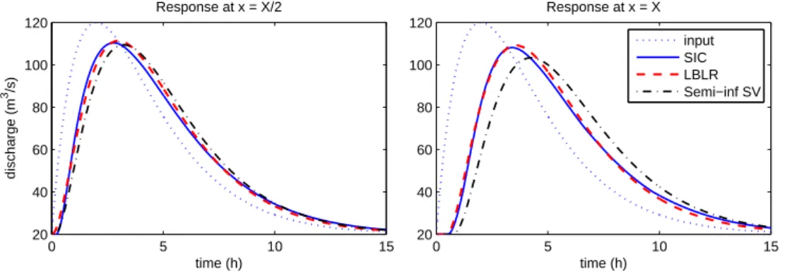
Two important characteristics of flood propagation are the attenuation level of the peak flow and the peak time. In this section, the previous example canal is considered with a weir at the downstream end. The weir is 80 m long, and 2 m high, with a discharge coefficient of 0.4. Eq. (12) is used to characterize the weir. The upstream discharge routed through the channel is defined as follows:

Q(0, t) = Qm+ (QM − Qm)

t T0

e1−T0t _{if t}≥ 0 ₍₃₈₎

where Qm = 20 m3/s and QM = 120 m3/s are the minimum and maximum

discharges respectively, and T0 = 2 h is the upstream time to peak. The

reference discharge is set to the mean value of the upstream discharge: Q = 56 m3_{/s. With the chosen downstream boundary condition, this leads to Y}

X =

1.92Ynand k = 2.21kn. Fig. 13 shows the response to the upstream hydrograph

at x = X/2 and x = X. 0 5 10 15 20 40 60 80 100 120 Response at x = X/2 time (h) discharge (m 3/s) 0 5 10 15 20 40 60 80 100 120 Response at x = X time (h) input SIC LBLR Semi−inf SV

Fig. 13. Simulation of the response in the time domain at x = X/2 and x = X.

The attenuation level is deﬁned as the diﬀerence between the upstream max-imum discharge and the maxmax-imum discharge at the abscissa x. Table 5 sum-marizes, for each simulation, the attenuation level and the peak time at the downstream end of the channel (x = X). The relative error with respect to SIC results is given in brackets.

(23)

Table 5

Attenuation level and peak time at x = X for each simulation. Relative error with respect to SIC results is given in brackets.

Model SIC LBLR Semi-inﬁnite

attenuation (m3/s) 11.9 10.8 (9.2 %) 16.7 (40.3 %) peak time (h) 3.42 3.57 (4.4 %) 4.26 (24.6 %)

For this realistic example case, accounting for the downstream boundary con-dition leads to a great improvement in the simulation of peak ﬂow attenuation. In addition, although the upstream discharge varies from 20 to 120 m3/s in this simulation, the linearization of the Saint-Venant equations seems to be still valid according to the good results obtained with the LBLR model. Let us also notice that the peak time is correctly reproduced by the LBLR model, while it is largely overestimated by the model which uses the semi inﬁnite assumption.

6.4 Criteria on the downstream boundary condition

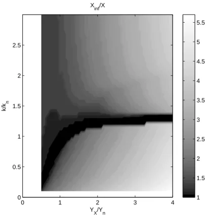
It is usual in the literature to perform simulation on longer river stretches in order to minimize the effects of the downstream boundary condition (see e.g. [4]). In that case, the semi-infinite canal is usually simulated with a three to five times longer canal. The LBLR model can be used to provide a quantification of this approximation. For instance, let us consider the response time (defined in section 6.1) for the example canal. We first estimate the response time at the distance x = ¯X = 10000 m calculated with the semi-infinite Saint-Venant

model and denoted RTsemi−inf. Then we vary the downstream water depth

YX and the feedback coeﬃcient k in the intervals [0.5Yn, 4Yn] and [0.1kn, 3kn],

respectively. Each couple (YX, k) represents a particular downstream boundary

condition. We expect that the response time at x = ¯X, denoted RTLBLR,

calculated with the LBLR model tends to RTsemi−inf when the length of the

canal X increases. We deﬁne the distance X_∞ as the minimum length X from which the relative error between RTsemi−inf and RTLBLR is lower than 5%.

Fig. 14 shows the evolution of X_∞/ ¯X with respect to YX/Yn and k/kn.

X_∞/ ¯X = 1 means that the downstream boundary condition has almost no

eﬀect on the dynamics. On the contrary, X_∞/ ¯X = 5 means that the length of

the canal has to be multiplied by 5 to ensure an error on the response time lower than 5%.

This graph shows that backwater effects as well as feedback effects can have a large impact on the dynamics. The black zone corresponds to the cases where those two effects are compensated, which means that the channel has quite the same behavior with or without the downstream boundary condition. One

(24)

Y X/Yn k/k n X inf/X 0 1 2 3 4 0 0.5 1 1.5 2 2.5 1 1.5 2 2.5 3 3.5 4 4.5 5 5.5

Fig. 14. Evolution of X_∞/ ¯X with respect to YX/Yn and k/kn.

may conclude that, even under normal ﬂow conditions (YX = Yn), feedback

effect can have an important impact on dynamics, especially for low values of the feedback coefficient k. The graph also leads to the other conclusion that for the particular value of k = 1.3kn, backwater effects have almost no impact

on the dynamics, as shown previously with the canal ended by a weir. For the ﬂood routing process, similar criteria can be built based on the calculation of the peak time or of the attenuation of the peak discharge.

7 Conclusion

The article proposes a new analytical and distributed model to approximate flow transfer for a non-uniform open-channel pool. The LBLR is a first- or second-order-with-delay transfer function that approximates the complete trans-fer matrix of the linearized Saint-Venant equations coupled with a downstream boundary condition. The model has been shown to efficiently reproduce the dy-namic behavior of an open-channel with backwater and different downstream boundary conditions.

The main advantages of this model are that it gives the discharge at any location in the channel depending on the discharge at the upstream end, it

(25)

integrates the ﬂow non-uniformity due to downstream hydraulic structures, and results are given as closed-form expressions, so quick computations are made possible.

Many applications are possible, from an accurate ﬂow routing to the estimation of the response time or the attenuation level in a prismatic open-channel, even in the case of large discharge variations. The research of equivalent geometric characteristics for non prismatic channels is under study. At the same time, this model remains simple enough to be used for controller design for open-channel, such as downstream PI controllers, or even for advanced controller design (e.g. multivariable controllers).

8 Acknowledgment

This work was jointly supported by Region Languedoc Roussillon and Cema-gref within the PhD thesis of Simon Munier, under the supervision of X. Litrico and G. Belaud.

References

[1] Balogun OS, Hubbard M, DeVries JJ. Automatic control of canal ﬂow using linear quadratic regulator theory. Journal of Hydraulic Engineering,

1988;114:75-102.

[2] Baume JP, Malaterre PO, Belaud G, Le Guennec B. SIC: a 1D Hydrodynamic Model for River and Irrigation Canal Modeling and Regulation. M´etodos Num´ericos em Recursos Hidricos, 2005;7:1-81.

[3] Becker A, Kundzewicz ZW. Nonlinear ﬂood routing with multilinear models.

Water Resources Research, 1987;23(6):1043-1048.

[4] Bentura PLF, Michel C. Flood routing in a wide channel with a quadratic lag-and-route method. Hydrological Sciences, 1997;42(2):169-189.

[5] Camacho LA, Lees MJ. Multilinear discrete lag-cascade model for channel routing. Journal of Hydrology, 1999;226(1-2):30-47.

[6] Chow V. Open-channel Hydraulics. McGraw-Hill Book Company, New York. 1988. 680 p.

[7] Chung WH, Aldama AA, Smith JA. On the effects of downstream boundary conditions on diffusive flood routing. Advances in Water Resources, 1993;16(5):259-275.

(26)

[8] Dooge J, Napi´orkowski J, Strupczewski W. The linear downstream response of a generalized uniform channel. Acta Geophysica Polonica, 1987a;XXXV(3):279-293.

[9] Dooge J, Napi´orkowski J, Strupczewski W. Properties of the generalized downstream channel response. Acta Geophysica Polonica, 1987b;XXXV(6):967-972.

[10] Garcia A, Hubbard M, DeVries JJ. Open channel transient ﬂow control by discrete time LQR methods. Automatica, 1992;28:255-264.

[11] Hurand, P. and Kosuth, P. R´egulations en rivi`ere. La Houille Blanche,

1993;2/3:143-149.

[12] Kundzewicz ZW. Multilinear ﬂood routing. Acta Geophysica Polonica,

1984;32(4):419-445.

[13] Litrico, X. Robust IMC ﬂow control of SIMO dam-river open-channel systems.

IEEE Trans. on Control Systems Technology, 2002;10:432-437.

[14] Litrico X, Fromion V. Frequency modeling of open channel ﬂow. Journal of

Hydraulic Engineering, 2004a;130(8):806-815.

[15] Litrico X, Fromion V. Simpliﬁed modeling of irrigation canals for controller design. Journal of Irrigation and Drainage Engineering, 2004b;130(5):373-383. [16] Litrico X, Fromion V. Boundary control of linearized Saint-Venant equations

oscillating modes. Automatica, 2006;42(6):967-972.

[17] Litrico, X. and Georges, D. Robust continuous-time and discrete-time ﬂow control of a dam-river system (I): Modelling & (II): Controller Design. Applied

Mathematical Modelling, 1999;23:809-827,829-846.

[18] Litrico X, Pomet JB. Nonlinear modeling and control of a long river stretch.

European Control Conference. 2003.

[19] Lundberg KH, Miller HR, Trumper DL. Initial conditions, generalized functions, and the Laplace transform: Troubles at the origin. IEEE Control

Systems Magazine, 2007;27(1):22-35.

[20] Malaterre, PO. Mod´elisation analyse et commande optimale LQR d’un canal d’irrigation. M. Sc. thesis, LAAS - CNRS - ENGREF - Cemagref. 1994. In French.

[21] Malaterre, PO. PILOTE: Linear quadratic optimal controller for irrigation canals. J. Irrig. Drain. Eng., 1998;124:187–194.

[22] Perumal M. Multilinear discrete cascade model for channel routing. Journal of

Hydrology, 1994;158(1-2):135-150.

[23] Rey J. Contribution à la modélisation et la régulation des transferts d’eau sur des systèmes de type rivière/baches intermédiaires. M. Sc. thesis, Université Montpellier 2. 1990. In French.

(27)

[24] Schuurmans J, Clemmens AJ, Dijkstra S, Hof A, Brouwer R. Modeling of irrigation and drainage canals for controller design. Journal of Irrigation and

Drainage Engineering, 1999;125(6):338-344.

[25] Strelkoﬀ TS, Deltour JL, Burt CM, Clemmens AJ, Baume JP. Inﬂuence of Canal Geometry and Dynamics on Controllability. Journal of Irrigation and

Drainage Engineering, 1998;124(1):16-22.

[26] Tsai CW. Applicability of kinematic, noninertia, and quasi-steady dynamic wave models to unsteady ﬂow routing. Journal of Hydraulic Engineering,

2003;129(8):613-627.

[27] Tsai CW. Flood routing in mild-sloped rivers-wave characteristics and downstream backwater eﬀect. Journal of Hydrology, 2005;308(1-4):151-167. [28] Weinmann P, Laurenson E. Approximate ﬂood routing methods: A review.

(28)

Appendix

A Computation of Saint-Venant Transfer Matrix

Applying Laplace transform to the linear partial diﬀerential Eqs. (2) and (3), and reordering leads to an ordinary diﬀerential equation in the variable x, with a complex parameter s (the Laplace variable):

d dx   q(x, s) y(x, s)   =As   q(x, s) y(x, s)    (A.1) with As =    0 −T s − s−µ T (C2_−V2₎ 2V T s+ν T (C2_−V2₎   

There are two boundary conditions q(0, s) in x = 0 and q(X, s) in x = X. Let us consider the integration of this linear system

dξs(x)

dx =Asξs(x) (A.2)

with ξs(x) = (q(x, s), y(x, s))T and where the initial condition is deﬁned at

x = 0. The solution of the system always exists and is given by:

ξs(x) = Γs(x)ξs0 =   γ11(x, s) γ12(x, s) γ21(x, s) γ22(x, s)   ξs0 (A.3)

where Γs(x) is the transition matrix and ξs0 the upstream condition at x = 0.

To solve this equation, let us diagonalize matrixAs:

As= PsDsPs−1

(29)

Ds=  λ1(s) 0 0 λ2(s)   , Ps= 1 T s   T s T s −λ1(s) −λ2(s)   , P_s−1= 1 λ1(s)− λ2(s)  −λ2(s) −T s λ1(s) T s   ,

and the eigenvalues:

λi= α + (−1)iβ, i = 1, 2 α = a + bs β =√(2ad + c2_)s2_{+ 2acs + a}2 with a = ν 2T (C2_−V2₎, b = V C2_−V2, c = V ν−(C2_−V2_{)T µ} ν(C2_−V2₎ , d = 1 2a [ C2 (C2_−V2₎2 − c2 ] .

In the uniform case, the transition matrix Γs(x) of (A.2) between 0 and x, is given

by the following closed-form expression ([14]):

Γs(x) = PseDsxPs−1=   λ1e λ2x_−λ_2eλ1x λ1−λ2 T s(e λ2x_−eλ1x) λ1−λ2 λ1λ2(eλ1x_−eλ2x₎ T s(λ1−λ2) λ1eλ1x_−λ2eλ2x λ1−λ2   (A.4)

Finally the solution of the ordinary diﬀerential Eq. (A.2) is:  q(x, s) y(x, s)   = Γ_s(x)  q(0, s) y(0, s)   (A.5)

B Taylor series expansion of the Saint-Venant transfer function

The method to obtain the Taylor series expansion of the Saint-Venant transfer function is detailed in this section.

(30)

B.1 Some preliminary computations

The elements of the transfer matrix Γ are expressed as functions of λ1 and λ2 or as functions of α and β. So writing the Taylor series of α and β leads to the Taylor series of the elements of Γ(x, s).

To make sure that no term will be forgotten in the computations, we choose to compute the fourth order Taylor series of α and β, given by:

α(s) = a + bs β(s) = a + cs + ds2−cd as 3₊ ( c2d a2 − d2 2a ) s4

In order to simplify the computations, we deﬁne three intermediate variables Z1x(s),

Z2x(s), Z3x(s). The following equations resume these variables and their Taylor series: Z1x(s) = e−2βx= A1x+ B1xs + C1xs2+ D1xs3+ E1xs4 (B.2) A1x = e−2ax B1x =−2cxe−2ax C1x =−2x ( d− c2x)e−2ax D1x =−4cx [ 1 3c 2_x2_{− 2ad}(_{1 +} x 2a )] e−2ax E1x = [( d2x a − 2 c2dx a2 ) (1 + 2ax)− 4c2dx3+ 2 3c 4_x4 ] e−2ax Z2x(s) = e(α+β)x= A2x+ B2xs + C2xs2+ D2xs3+ E2xs4 (B.3) A2x = e2ax B2x = (b + c)xe2ax C2x = ( dx +1 2(b + c) 2_x2 ) e2ax D2x = ( −cdx a + (b + c)dx 2₊1 6(b + c) 3_x3 ) e2ax E2x = [ c2_dx a2 − cdx2 a (b + c)− d2_x 2a (1− ax) + 1 2x 2_{(b + c)}2 ( dx + 1 12(b + c) 2_x2 )] e2ax Z3x(s) = α2− β2 T s = A3x+ B3xs + C3xs 2_{+ D} 3xs3+ E3xs4 (B.4)

(31)

A3x = 2 Ta(b− c) B3x = 1 T ( b2− c2− 2ad) C3x = 0 D3x = 0 E3x = 0

We also deﬁne two operators M and D. These operators are used to compute the Taylor series of the multiplication F1(s)F2(s) and the division F1(s)/F2(s), where

F1(s) = A1+ B1s + C1s2+ D1s3+ E1s4and F2(s) = A2+ B2s + C2s2+ D2s3+ E2s4. If FM =M(F1, F2) and FD =D(F1, F2) and if the Taylor series of FM(s) and FD(s)

are given by:

FM(s) = AM + BMs + CMs2+ DMs3+ EMs4

FD(s) = AD+ BDs + CDs2+ DDs3+ EDs4

then operators M and D give:

AM = A1A2 BM = A1B2+ B1A2 CM = A1C2+ B1B2+ C1A2 DM = A1D2+ B1C2+ C1B2+ D1A2 EM = A1E2+ B1D2+ C1C2+ D1B2+ E1A2 and AD = A1 A2 BD = 1 A2 ( B1− A1B2 A2 ) CD = 1 A2 [ C1− B1B2 A2 − A1 A2 ( C2− B₂2 A2 )] DD = 1 A2 [ D1− C1B2 A2 − B1 A2 ( C2− B2₂ A2 ) −A1 A2 ( D2− 2 B2C2 A2 + B 3 2 A2₂ )] ED = 1 A2 [ E1− D1B2 A2 − C1 A2 ( C2− B₂2 A2 ) −B1 A2 ( D2− 2 B2C2 A2 +B 3 2 A2 2 ) −A1 A2 ( E2− 2 B2D2+ C22 A2 + 3B 2 2C2 A2₂ − B₂4 A3₂ )]

We deﬁne a last intermediate variable δx(s) as following:

δx(s) =

1− e−2βx 2β e

(α+β)x₌ 1− Z1x

(32)

Knowing the Taylor series of Z1x and Z2x and using the two operatorsM and D, we can compute the Taylor series of the function δx(s):

δx(s) =M [D (1 − Z1x, 2β) , Z2x] (B.6)

B.2 Transfer Matrix Γ and Transfer Function T F

All the elements of the transfer matrix Γ(x, s) can be expressed from the four variables previously introduced.

γ11(x, s) = Z2x(s)− (α + β)δx(s) (B.7)

γ12(x, s) =−T sδx(s) (B.8)

γ21(x, s) = Z3x(s)δx(s) (B.9)

γ22(x, s) = Z2x(s) + (α− β)δx(s) (B.10)

So knowing the Taylor series of these intermediate variables, we can use the two operatorsM and D to compute the Taylor series of each γij(x, s).

γ11(x, s) = Z2x(s)− M (α + β, δx(s)) (B.11)

γ12(x, s) =−M (T s, δx(s)) (B.12)

γ21(x, s) =M (Z3x(s), δx(s)) (B.13)

γ22(x, s) = Z2x(s) +M (α − β, δx(s)) (B.14)

In the same way, we compute the Taylor series of γij(X, s).

Then it is possible to compute the Taylor series of k0(X, s) (Eq. (14)):

k0(X, s) =−D (γ12(X, s)− kγ22(X, s), γ11(X, s)− kγ21(X, s)) . (B.15)

Finally we get the Taylor series of T F (x, s) (Eq. (15)):

T F (x, s) = γ11(x, s) +D (γ12(x, s), k0(X, s)) (B.16)

One can remark that for s = 0, γ11(x, 0) = 1 and γ12(x, 0) = 0, which leads to

T F (x, 0) = A(x) = 1. This means that the static gain of the approximate transfer

function is equal to 1. This result is in agreement with the conservative property of the ﬂow.

(33)

C Taylor series expansion of the Saint-Venant transfer function in the non uniform case

In the non-uniform case, the reach is split into two sub-pools. Variables a, b, c, d,

x, X, T , α, β are replaced by their values corresponding to each sub-pool. In that

sense, matrix Γ(x, s) is replaced by Γ(x, s) and Γ(x, s) respectively, where x = x and

X = x1 are the relative position and the length of the uniform part, and x = x− x1 and X = X− x1 are the relative position and the length of the backwater part (x1 is the abscissa of the connection point).

The Taylor series of Γ(x, s) and Γ(x, s) are computed for each sub-pool (see appendix B). In the backwater part (x1 ≤ x ≤ X), the Taylor series of ˆΓ(x, s) is computed using operator M.

Then we can compute the Taylor series of ˆk0(X, s) (Eq. (34)): ˆ

k0(X, s) =−D (ˆγ12(X, s)− kˆγ22(X, s), ˆγ11(X, s)− kˆγ21(X, s)) . (C.1)

Finally we get the Taylor series of T F (x, s) (Eq. (33)):

T F (x, s) = ˆγ11(x, s) +D ( ˆ γ12(x, s), ˆk0(X, s) ) (C.2)

D Moment matching method

D.1 Second-order-with-delay

The transfer function T F is approximated by a second-order-with-delay:

q(x, s) = g(x)e

−τ(x)s

(1 + K1(x)s) (1 + K2(x)s)

q(0, s) (D.1)

We use the following property of the R-th cumulant MR (logarithmic moment) of

a function h(s) expressed in the Laplace domain:

MR[h(s)] = (−1)R

dR

dsR[log h(s)] (D.2)

(34)

Equating the cumulants of T F and its approximate form leads to:          M0(x) = log g(x) M1(x) = τ (x) + K1(x) + K2(x) M2(x) = K12(x) + K22(x) M3(x) = 2K13(x) + 2K23(x) (D.3) Let S = K1+ K2 and P = K1K2: S2= M2+ 2P (D.4) S3=M3 2 + 3P S (D.5)

which leads to the third order equation:

S3− 3M2S + M3 = 0 (D.6)

We can ﬁnd (u, v) such as u + v = S and uv = T . Then (D.6) leads to:

u3+ v3+ 3(T − M2)(u + v) + M3 = 0 (D.7)

If we choose T = M2, we obtain the following system:

u3+ v3=−M3 (D.8)

u3v3= M₂3 (D.9)

u3 and v3 are solutions of the second order equation:

X2+ M3X + M23 = 0 (D.10)

If M₃2 ≤ 4M₂3, the solutions of (D.10) are complex and this ensure the stability of the approximation by a second-order-with-delay. Otherwise the Saint-Venant transfer function can be approximated by a ﬁrst-order-with-delay. The system to be solved is then given by the ﬁrst three equations of the system (D.3) with K2= 0.

(35)

In the case where M₃2 < 4M₂3, the solution of (D.3) is given by:                                            ϕ = π 2 + arctan ( M3 √ 4M₂3− M₃2 ) S = 2√M2cos ϕ 3 P =−M2− M3 2S τ = M1− S K1 = S +√S2_{− 4P} 2 K2 = S−√S2− 4P 2 g = 1 (D.11) D.2 First-order-with-delay