Dynamic Greenland ice sheet driven by pCO2 variations across the Pliocene Pleistocene transition

HAL Id: hal-01945992

https://hal.sorbonne-universite.fr/hal-01945992

Submitted on 5 Dec 2018

HAL is a multi-disciplinary open access

archive for the deposit and dissemination of

sci-entific research documents, whether they are

pub-lished or not. The documents may come from

teaching and research institutions in France or

abroad, or from public or private research centers.

L’archive ouverte pluridisciplinaire HAL, est

destinée au dépôt et à la diffusion de documents

scientifiques de niveau recherche, publiés ou non,

émanant des établissements d’enseignement et de

recherche français ou étrangers, des laboratoires

publics ou privés.

Distributed under a Creative Commons Attribution| 4.0 International License

Dynamic Greenland ice sheet driven by pCO2 variations

across the Pliocene Pleistocene transition

Ning Tan, Jean-Baptiste Ladant, Gilles Ramstein, Christophe Dumas, Paul

Bachem, Eystein Jansen

To cite this version:

Ning Tan, Jean-Baptiste Ladant, Gilles Ramstein, Christophe Dumas, Paul Bachem, et al.. Dynamic

Greenland ice sheet driven by pCO2 variations across the Pliocene Pleistocene transition. Nature

Communications, Nature Publishing Group, 2018, 9, pp.4755. �10.1038/s41467-018-07206-w�.

�hal-01945992�

Dynamic Greenland ice sheet driven by pCO

₂

variations across the Pliocene Pleistocene

transition

Ning Tan

1,2

, Jean-Baptiste Ladant

1,3,4

, Gilles Ramstein

1

, Christophe Dumas

1

, Paul Bachem

5

& Eystein Jansen

6

It is generally considered that the perennial glaciation of Greenland lasting several orbital

cycles began around 2.7 Ma along with the intensification of Northern Hemisphere glaciation

(NHG). Both data and model studies have demonstrated that a decline in atmospheric pCO

2

was instrumental in establishing a perennial Greenland ice sheet (GrIS), yet models have

generally used simplistic pCO

2

constraints rather than data-inferred pCO

2

evolution. Here,

using a method designed for the long-term coupling of climate and cryosphere models and

pCO

2

scenarios from different studies, we highlight the pivotal role of pCO

2

on the GrIS

expansion across the Plio-Pleistocene Transition (PPT, 3.0

–2.5 Ma), in particular in the range

between 280 and 320 ppm. Good qualitative agreement is obtained between various IRD

reconstructions and some of the possible evolutions of the GrIS simulated by our model. Our

results underline the dynamism of the GrIS waxing and waning under pCO

2

levels similar to

or lower than today, which supports recent evidence of a dynamic GrIS during the

Plio-Pleistocene.

DOI: 10.1038/s41467-018-07206-w

OPEN

1_{Laboratoire des Sciences du Climat et de l’Environnement, LSCE/IPSL, CEA-CNRS-UVSQ, Université Paris-Saclay, 91191 Gif-sur-Yvette, France.}2_Key

Laboratory of Cenozoic Geology and Environment, Institute of Geology and Geophysics, Chinese Academy of Sciences, 100029 Beijing, China.3Département de Géosciences, École Normale Supérieure, Paris 75005, France.4_{LMD/IPSL, CNRS/ENS/UPMC, Ecole Polytechnique, Paris 75005, France.}5_{Uni Research}

Climate, Bjerknes Centre for Climate Research, Jahnebakken 5, 5007 Bergen, Norway.6_{Dep. of Earth Science, University of Bergen, Bjerknes Center for}

Climate Research, Jahnebakken 5, 5007 Bergen, Norway. Correspondence and requests for materials should be addressed to N.T. (email:ning.tan@mail.iggcas.ac.cn)

123456789

T

he long-term trend that led to the initiation of the cyclic

Northern Hemisphere glaciations (NHG) can be dated

from 3.6 Ma

1

_{. A set of reconstructed SST records}

2–4

_spread

across the globe describes a gradual cooling trend for the middle

to late Pliocene and early Pleistocene (3.6–2.2 Ma), associated

with a progressive increase in high

δ

18

_{O peaks of benthic}

for-aminifera

5

, reflecting both lower deep-water temperatures and

increased ice volume. Terrestrial data from Lake El’gygytgyn are

also consistent with long-term ocean cooling

6

_{. During this period,}

the

first marked peak of IRD was found around 3.4–3.3 Ma (MIS

MG2 and MIS M2) East of Greenland (ODP site 907

7

) and is

interpreted as evidence of an important glacial event occurring

before the establishment of the cyclic NHG around 2.7 Ma

7,8

_.

Significant amounts of IRD were recovered in different ocean

drilling sites in the North Atlantic during the PPT

9

. These

deposited IRD likely originated from Greenland, Iceland, North

America and Scandinavia, suggesting large land ice expansions to

the coast during this interval

7,9

. In addition, records based on

volcanic and sedimentary facies from Iceland also indicate the

onset of a large glaciation after 2.6 Ma

10,11

. The onset of a

per-ennial GrIS and of the cyclic NHG at the end of the PPT stands

out as a tipping point in the climate evolution of the Earth.

Indeed, it marks the beginning of a low pCO

2

world with

per-ennial ice sheets in both hemispheres, an infrequent occurrence in

the Earth’s history

12

_{, thereby creating specific geologic and}

cli-matic conditions allowing the development of glacial/interglacial

cycles.

Greenland, however, may have experienced waxing and waning

of ice before the intensification of NHG, as suggested by Eocene,

late Miocene and early Pliocene IRD records

13–15

. In particular,

the last large Northern Hemisphere glaciation prior to the major

intensification at 2.7 Ma occurred during MIS-M2 (3.312–3.264

Ma)

1,16–18

. This 50 kyrs glaciation was followed by the

well-established Mid-Pliocene Warm Period (MPWP) from 3.3 Ma to

3.0 Ma for which numerous observational and modelling studies

performed in the framework of the PlioMIP project

19

have

demonstrated that the warmer conditions led to a reduced

GrIS

20–22

_{(Supplementary Fig. 1). The subsequent build-up of a}

perennial GrIS across the PPT remains poorly constrained from a

spatio-temporal point of view due to its minor contribution to the

signal in global benthic foraminiferal

δ

18

_{O records and the}

paucity of direct geological data associated with the GrIS

expansion. Models have the potential to provide valuable insights

into the GrIS evolution but its transient nature remains

compli-cated to explore with fully coupled Global Climate Models

(GCM). Most climate/cryosphere studies on the GrIS onset

during the PPT using GCM have generally produced snapshot

climatic simulations subsequently used to force an ice sheet

model (e.g. ref.

23

). For instance, Lunt et al.

23

demonstrated,

based on a series of fully coupled GCM snapshot experiments

with different forcing factors, that pCO

2

decline was the major

driver of the GrIS glaciation. However, this result was obtained

from equilibrium simulations at 2.7 Ma and the underlying GCM

simulations included a pre-existent Pliocene GrIS

21

_{. A more}

recent study, also using snapshot simulations at 2.7 Ma,

demon-strated that pCO

2

values had to remain low to counterbalance the

increasing summer insolation in order to maintain the GrIS after

the initial onset

24

_{. In contrast, low resolution, conceptual and}

intermediate complexity models have been used to perform

transient long-term experiments

25–27

, but these models remain

simplified with respect to many processes and do not have the

spatial resolution to focus specifically on Greenland. Willeit

et al.

28

have recently worked on increasing the resolution but

their simulations of the GrIS across the PPT still used pre-defined

pCO

2

forcings. Therefore, although important insights into the

dynamics of the cryosphere across the PPT have emerged from

these studies, simulation of the GrIS evolution across PPT with a

forward physically-based model driven by realistic forcings

remains a major challenge. Here, we use a recent numerical

interpolation method

29

(see Methods), which couples climate

simulations obtained with the fully coupled IPSL-CM5A model

30

and the 15-km resolution version of the ice sheet model

GRI-SLI

31

, in order to investigate the transient evolution of the GrIS

across the PPT. The major advantage of our approach is the

ability to directly test the response of the climate-ice sheet system

to different pCO

2

evolution scenarios (see Methods) in order to

define plausible pCO

2

scenarios that led to the GrIS inception and

variability. We thus apply various reconstructions of pCO

2

evo-lution across the PPT from both proxy records and inverse

modelling studies (e.g. ref.

27,28,32–35

), as well as constant pCO

2

evolutions.

Results

GrIS sensitivity to constant pCO

2

scenarios. We

first present six

ice sheet experiments with constant pCO

2

values ranging from

220 to 405 ppmv using realistic orbital variations

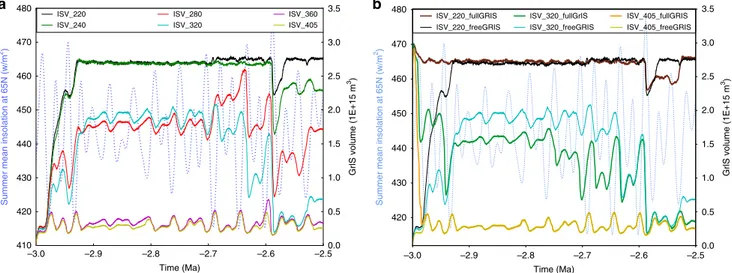
36

(Supplemen-tary Fig. 2b). As shown in Fig.

1

a, the evolution of the GrIS clearly

shows that below 280 ppmv of pCO

2

, it is possible to trigger and

maintain a large perennial ice sheet over Greenland even during

intervals of strong summer insolation, in particular around 2.6

Ma, whereas pCO

2

higher than 320 ppmv prevent the GrIS from

remaining perennial across the whole PPT period. Between 240

and 360 ppmv, the sensitivity of the GrIS volume to orbital

var-iations is considerable, illustrating the role of the complex

interplay between pCO

2

and orbital variations in the dynamics of

the GrIS, especially after 2.7 Ma when insolation becomes highly

variable. Finally for pCO

2

levels above 320 ppm, the ice sheet

extent remains limited across the whole 3–2.5 Ma interval. The

results of these constant simulations are in good agreement but go

one step beyond previous transient experiments at constant

pCO

237

in that we demonstrate that the GrIS possesses a

dyna-mism on orbital timescales across the PPT for only a narrow

range of atmospheric pCO

2

concentrations.

GrIS sensitivity to the initial boundary conditions. Existing

knowledge indicates that the GrIS largely retreated during the

MPWP, but the exact configuration of the Greenland ice sheet

and its topography remain highly uncertain

17

. In order to

investigate the impact of different initial states of the GrIS on its

subsequent evolution, we test two different initial boundary

conditions: an ice-free Greenland (Supplementary Fig. 1c) and

the modern GrIS (Supplementary Fig. 1a). We perform constant

pCO

2

simulations at three different levels (220 ppmv, 320 ppmv,

405 ppmv). Our results show that for extreme pCO

2

values (220

or 405 ppm) the simulated ice sheet evolution does not depend

upon the initial configuration of the ice sheet at 3.0 Ma (Fig.

1

b).

For pCO

2

levels closer to the modelled threshold for glaciation

(320 ppmv), orbital and pCO

2

forcings have comparable influence

on the simulated GrIS volume but these simulations demonstrate

that the initial configuration of the ice sheet also controls the GrIS

response. Indeed, bedrock vertical motion driven by the presence

or absence of ice can alter topography for tens or hundreds of

meters, which, at pCO

2

levels close to the threshold, may lead to

differences in ice volume and extent. However, the general

evo-lution of the GrIS volume remains similar in the scenario starting

with an ice-free Greenland and in that starting from a full ice

sheet. More importantly, during major deglaciation episodes

driven by high summer insolation, the modelled GrIS in both

cases recedes to identical configurations. As there is evidence for a

much reduced, perhaps even non-existent, GrIS during

inter-glacials of the MPWP (e.g., ref.

38,39

), we initialize the ice sheet

model with an ice-free Greenland. Indeed, the starting date of our

simulation (3 Ma) is preceded by a very high summer insolation

maximum (Supplementary Fig. 2b).

GrIS evolution using pCO

2

reconstructions. In the following,

we force our set-up with published reconstructions of

atmo-spheric pCO

2

, derived from recent proxy reconstructions

32–34

or

from inverse modelling

27,28,35

_{, in order to compare the modelled}

GrIS evolution to previous work and to IRD records across the

PPT.

We employ recent pCO

2

reconstructions based on alkenones

and boron measurements

32–34

(teal lines on Fig.

2

). These records

depict different pCO

2

evolution scenarios from a mostly linear

and low-resolution decrease for the older record

34

_to

high-resolution and high pCO

2

variations in the most recent record

33

.

When forced by the estimated high pCO

2

levels of Seki et al.

34

,

the GrIS evolution confirms the major role of orbital variations

when pCO

2

levels are confined to between ~280 ppmv and ~320

ppmv (Fig.

2

a). While pCO

2

levels remain above 350 ppm, even

large orbital variations do not significantly affect the extension of

the GrIS (3.0 to 2.9 Ma). During the 2.9–2.7 Ma interval, the low

variability in insolation prevents the GrIS from growing in spite

of pCO

2

levels dropping to 300 ppm. The simulated GrIS

evolution then shows a significant increase at 2.7 Ma and

pronounced orbital scale variability between 2.7 and 2.5 Ma, but

importantly, there is no full retreat of the GrIS during the

insolation maximum after 2.6 Ma because this maximum is

associated with pCO

2

levels below 300 ppm (Fig.

2

a). In contrast,

the Seki et al.

34

estimates of low pCO

2

levels generate a large

perennial GrIS as early as 2.9 Ma triggered by the combination of

an insolation minimum and low pCO

2

. A similar modelled

evolution of the GrIS is obtained when forced by the pCO

2

record

of Bartoli et al.

32

_{. Regardless of the uncertainties on the absolute}

values of pCO

2

concentration, the low levels in this record force

an early onset of a perennial GrIS (Fig.

2

b). However, because of

their low resolution, these two records do not show any pCO

2

variability on the ~10 kyrs timescale contrary to that of

Martinez-Boti et al.

33

, which demonstrates that the PPT pCO

2

evolution is

in fact much more variable than previously thought. The

uncertainties associated with the estimates of the Martinez-Boti

et al.

33

_{record show that a completely different evolution of the}

GrIS can be simulated (Fig.

2

c). The high (low) estimates depict

an evolution close to that driven by the high (low) estimates of

Seki et al.

34

, because the pCO

2

levels during times of insolation

extremes (3.0–2.9 Ma and 2.7–2.6 Ma) are similar. However, the

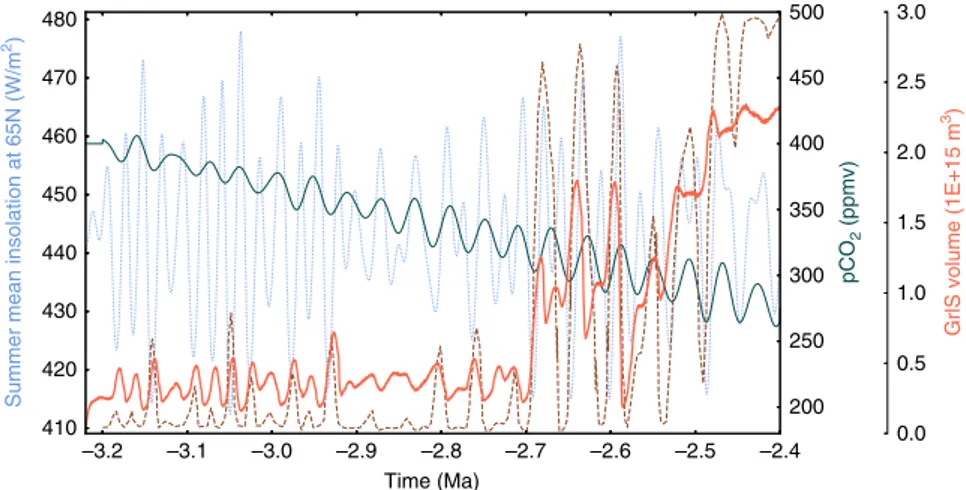
simulation forced with the mean pCO

2

estimates of

Martinez-Boti et al.

33

shows an early attempt of GrIS expansion

(~2.98–2.94 Ma) before a progressive onset from 2.8 Ma onwards,

with a significant increase in GrIS volume around 2.72 Ma and

2.6 Ma (Fig.

3

) because of the combination of low insolation and

low pCO

2

levels. After 2.6 Ma, the GrIS rapidly melts down to

small ice caps in the southern and southeastern margins (Figs

2

c

and

3

) because of a simultaneous increase in summer insolation

and pCO

2

. The ice sheet expansion then resumes at ~2.55 Ma (A

complete GrIS evolution with the mean pCO

2

estimates of

Martinez-Boti et al.

33

_{is shown in the Supplementary Movie 1).}

Interestingly, the pCO

2

records of Martinez-Boti et al.

33

generate

a sharp GrIS volume decrease after 2.6 Ma, regardless of the

uncertainties and earlier shape of the expansion of the ice sheet

because of an increase in pCO

2

values during the insolation

maximum. This seems contradictory to the presence of large and

perennial ice sheets from 2.7 Ma onwards but comparison with

IRD records

7,9

does not invalidate a scenario with a widescale

deglaciation after 2.6 Ma.

When forced by the monotonously decreasing and obliquity

modulated pCO

2

scenario defined by Willeit et al.

28

, our

simulated GrIS shows a similar evolution to that of Willeit

et al.

28

_(Fig.

₄

_{), in particular in the large increases in GrIS volume}

reproduced at 2.7 Ma and 2.55 Ma, as well as the large decrease at

2.6 Ma, although our GrIS volume displays less variability because

of a lower sensitivity to the orbital forcing in our fully coupled

climate-ice sheet model. Inverse modelling studies

27,35

_{have also}

provided potential pCO

2

reconstructions for this interval

(Supplementary Fig. 3). However, the low pCO

2

concentrations

throughout most of these reconstructions lead to a large perennial

GrIS even during the well-established MPWP warming period

19

,

in contrast to evidence for a much reduced GrIS

38,39

.

Discussion

In this work, we restrict high-resolution ice sheet modelling to

scenarios of the GrIS evolution across the PPT although much

evidence for ice growth outside Greenland has been reported

during this period

8,40,41

_{. This decision is warranted because}

Greenland is one of the primary location for ice nucleation in the

480

a

b

ISV_220 ISV_240 ISV_280 ISV_320 ISV_360 ISV_220_fullGRIS ISV_220_freeGRIS ISV_320_fullGrIS ISV_320_freeGRIS ISV_405_fullGRIS ISV_405_freeGRIS ISV_405 470 460 450 440

Summer mean insolation at 65N (w/m

2) 430 420 410 480 470 460 450 440

Summer mean insolation at 65N (w/m

2) 430 420 –3.0 –2.9 –2.8 Time (Ma) –2.7 –2.6 –2.5 –3.0 –2.9 –2.8 Time (Ma) –2.7 –2.6 –2.5 0.0 0.5 1.0 GrlS volume (1E+15 m 3) 1.5 2.0 2.5 3.0 3.5 0.0 0.5 1.0 GrlS volume (1E+15 m 3) 1.5 2.0 2.5 3.0 3.5

Fig. 1 Sensitivity tests with constant pCO2scenarios.a Simulated GrIS volume (ISV on thefigure) with various constant pCO2concentrations (220 ppmv,

240 ppmv, 280 ppmv, 320 ppmv, 360 ppmv, 405 ppmv; so that ISV_220 indicates the simulated GrIS with constant pCO2of 220 ppmv).b Simulated GrIS

volume with the three pCO2concentrations (220 ppmv, 320 ppmv and 405 ppmv under two different initial GrIS configurations: the present-day full GrIS

80°N

a

b

c

d

4 2.6 Ma 2.72 Ma 3 2.8 Ma 2 2.9 Ma 1 75°N 70°N 65°N 60°N 50°W 40°W 30°W 50°W 40°W 30°W 50°W 40°W 30°W 50°W 40°W 30°W 80°N 75°N 70°N 65°N 60°N 80°N 75°N 70°N 65°N 60°N 80°N 4000 3500 3000 2500 2000 m 1500 1000 500 75°N 70°N 65°N 60°N

Fig. 3 Greenland ice sheet thickness snapshots in the modelled GrIS evolution. These snapshots are taken from the simulated GrIS evolution based on the pCO2record of Martinez-Boti et al.33(mean) at 2.9 Ma (a), 2.8 Ma (b), 2.72 Ma (c) and 2.6 Ma (d), as shown on Fig.2c

480

b

a

c

500 3.0 2.5 2.0 1.5 1.0 0.5 0.0 3.0 2.5 2.0 1.5 1.0 0.5 0.0 3.0 2.5 2.0 1.5 1.0 0.5 0.0 450 400 350 300 250 200 500 450 400 350 pCO2 (ppmv)

GrIS volume (1E+15 m

3) 300 250 200 500 450 400 350 300 250 200 470 460 450 440 430 420 410 –3.0 –2.9 –2.8 –2.7 –2.6 –2.5 –3.0 –2.9 –2.8 –2.7 –2.6 –2.5 –3.0 –2.9 1 2 3 4 –2.8 Time (Ma) –2.7 –2.6 –2.5 480 470 460 450 440

Summer mean insolation at 65N (W/m

2) 430 420 410 480 470 460 450 440 430 420

Fig. 2 Simulated GrIS volume evolution based on different pCO2records.a Seki et al.34;b Bartoli et al.32;c Martinez et al.33. Dashed light blue line

represents the boreal summer insolation at 65°N. Orange lines are the simulated GrIS volumes based on pCO2records and their uncertainties, represented

by the solid teal lines and shaded teal areas.a Alkenone-based pCO2record of Seki et al.34, determined using size-correctedε37:2values for the modern

range ofb-values34_{. The solid (dashed) orange line is the simulated GrIS volume obtained with the solid (dashed) pCO}

2line.b Boron isotopes-based pCO2

record of Bartoli et al.32_{, with a 2σ error range. The solid orange line is the simulated GrIS volume with mean pCO}

2values and shaded orange lines are the

GrIS volumes obtained with low and high extremes of the pCO2uncertainties.c As in b but for the boron isotopes-based pCO2record of Martinez-Boti

et al.33_{, with an uncertainty range corresponding to 68% of 10,000 Monte Carlo simulations with full propagation of uncertainties}33_{. Circled numbers at}

2.9 Ma, ~2.8 Ma, ~2.72 Ma and 2.6 Ma correspond to the ice sheet snapshot displayed in Fig.3

North Hemisphere

15

and because there is currently no agreement

on the possible extent and configuration of possible ice sheets

outside Greenland. However, this restriction hampers

compar-isons with

δ

18

O and sea level records because the maximum ice

volume that can be accommodated over Greenland represents

roughly 7 m of equivalent sea level, i.e. in the range of

experi-mental and/or instruexperi-mental errors. Significant insights can

however be gained from adjacent IRD records

9

in order to further

constrain the possible evolution of the GrIS and of pCO

2

across

the PPT. It should be kept in mind that attempting to constrain

the GrIS geometry and volume from IRD records remains

spec-ulative because the absence of IRDs does not necessarily correlate

with the absence of GrIS and because IRD peaks may contain

material derived from other sources than the melting Greenland

icebergs. In addition, iceberg trajectories may change and the

ambient temperature along the iceberg trajectory may influence

the melt-out rates of the IRD contained in the icebergs. For

instance, variations in North Atlantic SST and/or currents or

changes in the sediment contents of the calved icebergs could

explain the absence of IRD even if the GrIS maintains a

sig-nificant iceberg discharge

41,42

_{. In addition, IRD peaks may}

represent an ice growth phase, during which increasing GrIS

volume could lead to increased iceberg discharge, as well as an ice

melt phase, during which the warmer climatic conditions could

lead to enhanced ice sheet melting and, consequently, enhanced

ice

flux at the margin. Despite these uncertainties, IRD records

offer a

first-order insight into ice sheet dynamics and their

rela-tionship to orbital variations, which may aid in defining the most

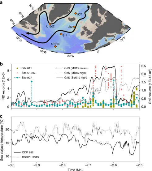
probable scenario for GrIS evolution. We used ODP Site 907

7

_,

IODP Site U1307

43

and ODP Site 611

41

(Fig.

5

. More details

about these data can be found in Supplementary Note 1) because

the IRD records from these sites can be confidently assumed to

originate primarily from the GrIS

41

. Sites U1307 and 907 are

located offshore from Greenland margins and show small but

continuous IRD deposition from as early as 3 Ma (Fig.

5

b), with

the exception of a single peak at 2.92 Ma at Site 907. Around 2.7

Ma, several IRD peaks in both records suggest intensification of

the iceberg discharge, broadly correlated to North Atlantic sea

surface temperatures (SST) cooling events (Fig.

5

c). Accordingly,

the record from Site 611, located further south from Greenland,

shows an absence of IRD deposition before 2.72 Ma and several

peaks afterwards.

There is variable agreement between our reconstructed GrIS

volume scenarios and inferred GrIS extension as implied by IRD

records. For instance, the GrIS evolution forced by the pCO

2

record of Bartoli et al.

32

agrees poorly with the IRD records

because it suggests a large to near-complete perennial GrIS as

early as 2.98–2.95 Ma (Fig.

2

b). Around 2.9 Ma, a large ice sheet

covering the totality of the southern Greenland margin is present

in the results forced by the pCO

2

records of Bartoli et al.

32

.

However, there are not any particular changes above the 3.0–2.7

Ma background IRD values at Site U1307. At Site 907, an early

increase of a large GrIS could explain the 2.92 IRD peak, but in

this case the IRD deposition should have continued with higher

levels relative to the pre-glaciation interval. In addition, the

absence of any IRD at Site 611 at that time suggests that the GrIS

was still of relatively limited size. In contrast to the pCO

2

record

of Bartoli et al.

32

_{, the mean and high pCO}

2

estimates of

Martinez-Boti et al.

33

_{and the high estimate of Seki et al.}

34

_{generate GrIS}

evolutions more consistent with the IRD records. The modelled

GrIS using these reconstructions is limited to small ice caps on

the southern and southeastern margins of Greenland during the

interval 3.0–2.7 Ma interval, which agrees well with small but

continuous IRD inputs at Site 907 and U1307 (Fig.

2

a, c, Fig.

3

and Fig.

5

a, b). The sharp increase in IRD deposition at 2.7 Ma is

also accounted for by these GrIS evolution scenarios.

Further-more, the IRD records of Site 611

41

displays four IRD peaks (at

~2.7 Ma, ~2.64 Ma, ~2.6 Ma and ~2.52 Ma) that are relatively well

correlated in time with decreases in North Atlantic SSTs and large

modelled GrIS variations (Fig.

5

b, c), in particular for the

Martinez-Boti et al.

33

_{mean and high pCO}

2

scenario. Importantly,

the large GrIS volume decrease after 2.6 Ma in these scenarios is

not at odds with the IRD records, in that the minimal GrIS state

still reaches the southern and southeastern margins of Greenland,

allowing small but uninterrupted iceberg discharge at Site 907.

These three pCO

2

scenarios (Martinez et al.

33

high, mean and

Seki et al.

34

high pCO

2

estimates) therefore seem to correlate

relatively well with IRD records because the GrIS expands

pre-ferentially from the south and east regions and intervals of large

GrIS variations are synchronous with IRD peaks.

There is evidence however showing that after 2.7 Ma, ice sheets

were not restricted to Greenland (e.g., ref.

40,41

). Although by

model design ice growth in other regions of the Northern

Hemisphere is not simulated, simple inferences of the impact of

North American and Scandinavian ice sheets after 2.7 Ma would

tend to suggest that the large GrIS retreat around 2.6 Ma might

have been more limited. Indeed, the cooling effects of such ice

masses on regional and global climate would presumably have

partly counterbalanced the combined increase in pCO

2

and

summer insolation. Still, the evidence for other NH ice sheets can

tentatively be used to suggest that the GrIS evolution driven by

the Martinez-Boti et al.

33

mean pCO

2

estimates is the most

480 500 3.0 2.5 2.0 1.5 1.0 0.5 0.0 450 400 350 pCO 2 (ppmv) GrlS volume (1E+15 m 3) 300 250 200 470 460 450 440

Summer mean insolation at 65N (W/m

2) 430 420 410 –3.2 –3.1 –3.0 –2.9 –2.8 Time (Ma) –2.7 –2.6 –2.5 –2.4

Fig. 4 Simulated GrIS volume evolution with the pre-de_{fined best scenario of pCO}2from Willeit et al.28. The brown dash line represents the GrIS evolution

of Willeit et al.28_{under the same pCO}

plausible pCO

2

scenario among those that are the most consistent

with IRD records (i.e. Martinez-Boti et al.

33

mean and high, Seki

et al.

34

_{high estimates), because it leads to a much larger GrIS}

between 2.8 and 2.6 Ma (Fig.

2

c). The presence of ice sheets over

North America and Scandinavia after 2.7 Ma is thus likely to be

more consistent with a largely or fully glaciated Greenland

because ice preferentially nucleates on Greenland before

poten-tially expanding over other regions of the Northern Hemisphere.

In conclusion, modelling the GrIS evolution across the PPT

using a recent method specifically designed for transient ice sheet

experiments shows that the long-lasting paradigm explaining the

large GrIS onset occurring at 2.7 Ma due to a minimum of

summer insolation at 65°N is, by far, too simplistic. In our

simulations, the GrIS volume appears very sensitive to pCO

2

changes during the PPT interval. Our experiments demonstrate

that pCO

2

levels have to remain below 320 ppmv in order to

develop and maintain perennial large GrIS across the whole PPT

interval, although the absolute pCO

2

values may be model

dependent. When forced by the most recent pCO

2

reconstruction

available

33

_{for this interval, the simulated GrIS shows a good}

agreement with IRD records from adjacent locations

7,41,43

. The

evolution of the GrIS across the PPT under this pCO

2

scenario

shows large variations of ice volume of continent-sized amplitude

but indicates a continuous presence of ice even during intervals of

higher pCO

2

and stronger summer insolation. This result

sup-ports recent work suggesting a very dynamic, yet persistent GrIS

for the last millions of years

44

_{, possibly receding to very small ice}

centres

45

. Ultimately, our work emphasizes the crucial role of

pCO

2

in shaping the evolution of the cryosphere across the PPT

and provides numerical arguments for a vigorously dynamic GrIS

under pCO

2

levels similar to, or lower than modern values.

Methods

Model description. The climate model used in this study is the IPSL-CM5A GCM30_{. The atmosphere component is the LMDZ5A version of the LMDz model}

(including the ORCHIDEE land-surface model) with a resolution of 3.75°×1.875° and 39 vertical layers. More details about the physical parameterization can be found in30,46_{. The ocean model is NEMOv3.2}47_{, which integrates the dynamical}

model OPA, the LIM2 sea ice model and the PISCES biogeochemical model. NEMO runs on a tri-polar grid (one pole in the Southern Hemisphere under Antarctica and two poles in the Northern Hemisphere under North America and Asia) in order to improve the representation of ocean dynamics in the northern high-latitudes. There are 31 unequally spaced vertical levels and a nominal reso-lution of 2° that is refined up to 0.5° in the equatorial area. The atmosphere and ocean models are linked through the coupler OASIS48_{, ensuring energy and water}

conservation. Additional details about the IPSL-CM5A model can be found in Dufresne et al.30_.

The ice sheet model used in this study is the GRenoble Ice-Shelf and Land-Ice model (GRISLI). GRISLI is a three-dimensional thermo-mechanical model that

8

a

b

c

Site 611 U1313 611 U1307 982 907 60°W 40°N 50°N 60°N 40°W 20°W 0° 20°E Site U1307 Site 907 ODP 982 DSDP U1313 GrlS (MB15 mean) GrlS (MB15 high) GrlS (Seki10 high) 2.5 2.0 1.5 1.0 0.5 GrlS volume (1E+15 m 3) 0.0 6 4

IRD records (1E+3)

Sea surface temperature (°C)

2 0 20 15 10 –3.0 –2.9 –2.8 Time (Ma) –2.7 –2.6 –2.5

Fig. 5 The comparison between the simulated GrIS and adjacent IRD records. a Map showing simpli_{fied main ocean currents in NATL and the ocean deep} drilling sites referenced in this study (Ocean Data View, Schlitzer, R., Ocean Data View, odv.awi.de, 2018).b Related IRD records in the North Atlantic regions: site 9077_{; site U1307}43_{; site 611}41_{and simulated GrIS volume with the mean and high pCO}

2estimates of Martinez-Boti et al.33and the high pCO2

estimate of Seki et al.34;c Reconstructed sea surface temperature at ODP site 982 by Lawrence et al.2and IODP site U1313 by Naafs et al.63

simulates the evolution of ice sheet geometry (extension and thickness) and the coupled temperature–velocity fields in response to climate forcing. A

comprehensive description of the model can be found in ref.31_{and ref.}49_{. In this}

study, the GRISLI model is nested to the Greenland region on a cartesian grid of 15 km × 15 km. Over the grounded part of the ice sheet, the iceflow resulting from internal deformation is governed by the shallow-ice approximation50_{. The model}

also deals with iceflow through ice shelves using the shallow-shelf approximation51

and predict the large-scale characteristics of ice streams using criteria based on the effective pressure and hydraulic load. At each time step, the velocity and vertical profiles of temperature in the ice are computed, as well as the new geometry of the ice sheet. The isostatic adjustment of the bedrock in response to the ice load is governed by theflow of the asthenosphere, with a characteristic time constant of 3000 years, and by the rigidity of the lithosphere. The temperaturefield is computed both in the ice and in the bedrock by solving a time-dependent heat equation. Here, as the ice sheet model GRISLI is not synchronously coupled with the IPSL-CM5A model, temperature and precipitationfields are asynchronously passed from IPSL-CM5A to GRISLI. The surface mass balance is defined as the sum between accumulation and ablation computed by the positive degree-day (PDD) method52_.

Interpolation method. In the absence of synchronous coupling between GRISLI and IPSL-CM5A, we utilise an interpolation that asynchronously couples both models and offers the possibility of carrying long-term numerical integration of the ice sheet model while accounting for the time evolution of the main climate for-cings. This method consists of building a matrix of possible climate states that are generated by IPSL-CM5A under various combinations of forcings, which are chosen from the range of possible values taken by forcings. The ice sheet model GRISLI can then be continuously forced by temperature and precipitationfields obtained by interpolation between the different IPSL-CM5A climatic states, interpolation based on the time evolution of the forcings. The principle of this method has been described in details in Pollard (2010) and an early version of it has been applied to the Eocene-Oligocene Transition (EOT) in Antarctica53_{. In this}

work, we use an improved version of this method, which hasfirst been applied to the EO glaciation29_{and that we have adapted to Greenland. Specifically here, we}

build a three-dimensional matrix to account for the three main drivers of an ice sheet evolution that are: (1) realistic insolation variations, (2) the atmospheric pCO2evolution and (3) the ice sheet feedbacks on itself. The matrix hence

com-prises temperature and precipitationfields that are obtained from reference IPSL-CM5A runs initialized with different combinations of orbital parameters, pCO2

and ice sheet size. In a second step, the temperature and precipitationfields that force GRISLI can be computed by interpolating between the reference IPSL-CM5A climatic states, based on the current value taken by the 65°N summer insolation and by the atmospheric pCO2and on the instantaneous size of the ice sheet in

GRISLI. This ensures that the climaticfields passed to GRISLI are appropriately updated at each time step to follow the evolution of both external (insolation and pCO2) and internal (ice sheet geometry) forcings.

Experiment design. In this study, we have chosen two orbital configurations that produce respectively the maximal (warm orbit) and the minimal (cold orbit) mean summer insolation at 65°N between 3.0 and 2.5 Ma, according to the astronomical solution calculated by the model of ref.36_{. At each time step of the ice sheet model}

simulations for the 3–2.5 Ma period, the impact of the summer insolation can be included by appropriately interpolating between reference IPSL-CM5A runs with warm or cold orbits.

The reference IPSL-CM5A runs are initialised with four different pCO2

concentrations: 220 ppmv, 280 ppmv, 360 ppmv and 405 ppmv. Late Pliocene pCO2records indeed document a range of variation of the atmospheric pCO2

comprised between ~200 ppmv and ~400 ppmv (See in Supplementary Fig. 2). Similarly, the instantaneous value of pCO2over the course of the simulation for the

3–2.5 Ma periods can be interpolated between reference runs with aforementioned pCO2values. As pCO2and temperature are linked via a logarithmic relationship,

we prescribe a logarithmic interpolation betweenfixed pCO2reference runs.

Conversely, the interpolation is kept linear for the insolation.

To obtain the reference Greenland ice sheet sizes that are prescribed in the reference IPSL-CM5A runs, we carry out a preliminary experiment in which we model the ice sheet development in an offline, one-way regrowth experiment (see ref.24_{for details). We initialise IPSL-CM5A with standard PlioMIP phase 1}

conditions54_{, which are then modified to start from an ice-free Greenland and}

extremely favourable conditions for glacial inception represented by the cold orbit described above and a pCO2concentration of 220 ppmv. GRISLI is then force with

constant temperature and precipitationfields from the IPSL-CM5A simulation until the ice sheet reaches equilibrium. The ice sheet geometry is then fed back to IPSL-CM5A while pCO2and orbital parameters are kept identical. New climatic

fields are thus obtained and GRISLI further simulates the ice sheet gain until a new equilibrium is reached. The geometry of the ice sheet can then be passed again to IPSL-CM5A. This process is repeated until a new iteration does not markedly increase the ice volume. Here, seven iterations allow us to obtain seven Greenland ice sheet sizes ranging from very small to nearly full size ice sheet (Supplementary Fig. 1c‒i).

The matrix of reference IPSL-CM5A climatic states is then built using the forcings described above. A total of 2 (for the insolation) × 4 (for pCO2) × 7 (for

Greenland ice sheet sizes) simulations are run in parallel to provide reference T and Pfields that cover the range of possible variations of the three main drivers that are insolation, pCO2and ice sheet size. A continuous T and P forcing can then be

calculated based on the prescribed (for insolation and pCO2) and emerging (for ice

sheet) evolutions of these drivers. Although complex and fastidious to implement, one particular advantage of this method is that it allows virtually any pCO2

scenario to be tested without additional GCM runs.

It should be noted that vegetation feedbacks linked to vegetation changes under Late Pliocene conditions are taken into account in our IPSL-CM5A simulations, since the tundra-taiga feedback has been shown to play a role in the onset of NH glaciation20_{. We divide the IPSL-CM5A boundary conditions into three types}

relative to their presumed impact on vegetation: cold, intermediate and warm. The cold conditions are defined by the combination of the cold orbit and either 220 ppmv or 280 ppmv of pCO2concentration. In the reference IPSL-CM5A

simulations whose boundary conditions fall under the cold criterion, we modify the PlioMIP vegetation map55_{by specifying tundra north of 50°N. The intermediate}

conditions are defined by the combination of the cold orbit and either 360 ppmv or 405 ppmv of pCO2concentration and the PlioMIP vegetation map is modified by

specifying tundra north of 65°N. Finally, the warm conditions are defined by the warm orbit, regardless of the pCO2concentration. Under these conditions, we keep

the PlioMIP vegetation map unchanged. All the reference AOGCM experiments are summarized in Supplementary Table. 1.

Model evaluation. We assess our model performances and our modelling strategy by presentingfirst a comparison between the simulated surface mass balance (SMB) obtained from the CMIP5 historical IPSL-CM5A experiment30_and

aver-aged over the period 1981–2005 and the SMB computed with the state-of-the-art regional polar model MAR56_{forced by reanalyses over the same interval. Second,}

we present a sensitivity experiment of the Eemian deglaciation (150–110 Ka) in which the pCO2evolution is very well constrained.

Supplementary Fig. 4 shows that the simulated SMB with our climate model IPSL-CM5A is consistent with the reconstructed SMB from MAR, except in some regions of the northwest and southeast Greenland. These differences can be attributed: (1) to the coarser resolution of IPSL-CM5A compared to MAR, which provide some limitations in the model’s ability to accurately simulate precipitation in mountainous regions (a common problem in fully coupled climate models, see e.g. ref.57_{), such as South Greenland here; 2) to biases in simulated temperatures}

and precipitations in the Greenland region in IPSL-CM5A30_{and/or MAR. Yet}

overall, the simulated SMB using IPSL-CM5A is reasonably close to that of MAR. In order to simulate the Eemian deglaciation, we have performed four additional climate simulations with a LGM ice sheet configuration, two low pCO2

scenarios (185 ppmv and 220 ppmv) and our two extreme orbital configurations. We also restrict the ice sheet simulation to Greenland. Because the climate states added in the matrix have extensive ice sheet and sea ice covers over the Northern Hemisphere, we allow the ice sheet model to use variable basal melting factors following the multi-proxy index of Quiquet et al.58_{. Basal melting factors thus vary}

linearly between 0 and 5 m/year in regions where depth are lower than 1300 m and arefixed to 10 m/year where depth greater than 1300 m. In addition, we use the sea level curve of Waelbroeck et al.59_{as a forcing to determine which ice model grid}

points arefloating or grounded. These two processes are added to take into account the climatic influence of the LIG deglaciation outside Greenland because we do not explicitly model this ice sheet evolution. Finally, the ice sheet model is initialized with the LGM GrIS.

The results from this sensitivity experiment are shown on Supplementary Fig. 5. The combined increase in summer insolation and pCO2leads to the waning of the

GrIS between 133 and 123 Ka. The timing of the deglaciation is consistent with results from other studies (e.g., ref.60–62_{). Stone et al.}60_{“best score” simulation}

places the start of the GrIS deglaciation at 135 Ka (their Fig. 6b, black lines) and the end around 123 Ka. Goelzer et al.62_{restrict theirfigures to the interval 130–115 Ka}

so that the start of the deglaciation in their simulations is unclear but the lowest GrIS volume is also found around 123 Ka. Finally, Bradley et al.61_{also place the}

beginning and end of the GrIS deglaciation at 133 and 123 Ka, respectively (their Fig.2). The contribution of the GrIS to sea level rise during the LIG is poorly constrained and estimated between 0.6 and 3.5 m61_{. Our simulated minimal GrIS}

reaches a volume of 2.846 × 1015_{km3 (Supplementary Fig. 6), which is slightly less}

than the equilibrium GrIS volume (2.87 × 1015_{k m3) simulated by GRISLI under}

preindustrial IPSL-CM5A forcings30_{. Compared to other studies, our simulated}

LIG GrIS does not reach a volume low enough. However, considering that we just adapted a method that is designed for the PPT and not specifically for the Eemian, we argue that the model does a reasonable job in reproducing the Eemian deglaciation. In summary, the reasonable agreement between our modelled deglaciation and the results from other transient LIG simulations provides confidence in our modelling strategy.

Code availability. The codes of the IPSLCM5 and GRISLI models are available on request to the authors.

Data availability

Data that support the results of this study are available on request to the authors.

Received: 17 January 2018 Accepted: 10 October 2018

References

1. Mudelsee, M. & Raymo, M. E. Slow dynamics of the Northern Hemisphere glaciation. Paleoceanography 20, 4022–4036 (2005).

2. Lawrence, K. T., Herbert, T. D., Brown, C. M., Raymo, M. E. & Haywood, A. M. High-amplitude variations in north atlantic sea surface temperature during the early pliocene warm period. Paleoceanography 24, 1–15 (2009). 3. Herbert, T. D., Peterson, L. C., Lawrence, K. T. & Liu, Z. Tropical ocean

temperatures over the past 3.5 million years. Science 328, 1530–1534 (2010). 4. Venti, N. L., Billups, K. & Herbert, T. D. Increased sensitivity of the

Plio-Pleistocene northwest Pacific to obliquity forcing. Earth Planet. Sci. Lett. 384, 121–131 (2013).

5. Lisiecki, L. E. & Raymo, M. E. A Pliocene-Pleistocene stack of 57 globally distributed benthicδ18_{O records. Paleoceanography 20, 1003–1020}

(2005).

6. Brigham-Grette, J. et al. Pliocene warmth, polar amplification, and stepped Pleistocene cooling recorded in NE Arctic Russia. Science 340, 1421–1427 (2013).

7. Jansen, E., Fronval, T., Rack, F. & Channell, J. E. T. Pliocene-Pleistocene ice rafting history and cyclicity in the Nordic Seas during the last 3.5 Myr. Paleoceanography 15, 709–721 (2000).

8. Maslin, Ma, Li, X. S., Loutre, M. F. & Berger, A. The contribution of orbital forcing to the progressive intensification of Northern Hemisphere glaciation. Quat. Sci. Rev. 17, 411–426 (1998).

9. Flesche Kleiven, H., Jansen, E., Fronval, T. & Smith, T. M. Intensification of Northern Hemisphere glaciations in the circum Atlantic region (3.52.4 Ma) -Ice-rafted detritus evidence. Palaeogeogr. Palaeoclimatol. Palaeoecol. 184, 213–223 (2002).

10. Eiriksson, J. & Geirsdóttir, Á. A record of Pliocene and Pleistocene glaciations and climatic changes in the North Atlantic based on variations in volcanic and sedimentary facies in Iceland. Mar. Geol. 101, 147–159 (1991).

11. GEIRSDÓTTIR, Á. & EIRiKSSON, J. O. N. Sedimentary facies and environmental history of the Late-glacial glaciomarine Fossvogur sediments in Reykjavík, Iceland. Boreas 23, 164–176 (1994).

12. Ramstein, G. Climates of the Earth and cryosphere evolution. Surv. Geophys. 32, 329 (2011).

13. Thiede, J. et al. Million years of Greenland Ice Sheet history recorded in ocean sediments. Polarforschung 80, 141–149 (2011).

14. Jansen, E. & Sjøholm, J. Reconstruction of glaciation over the past 6 Myr from ice-borne deposits in the Norwegian Sea. Nature 349, 600–603 (1991). 15. Larsen, H. C. et al. Seven million years of glaciation in Greenland. Science 264,

952–955 (1994).

16. De Schepper, S. et al. Northern hemisphere glaciation during the globally warm early Late Pliocene. PLoS ONE 8, e81508 (2013).

17. Dolan, A. M. et al. Modelling the enigmatic Late Pliocene Glacial Event -Marine Isotope Stage M2. Glob. Planet. Change 128, 47–60 (2015). 18. Tan, N. et al. Exploring the MIS M2 glaciation occurring during a warm and

high atmospheric CO2Pliocene background climate. Earth Planet. Sci. Lett.

472, 266–276 (2017).

19. Haywood, A. M. et al. On the identification of a Pliocene time slice for data-model comparison. Philos. Trans. A Math. Phys. Eng. Sci. 371, 1–21 (2013).

20. Koenig, S. J., DeConto, R. M. & Pollard, D. Late Pliocene to Pleistocene sensitivity of the Greenland Ice Sheet in response to external forcing and internal feedbacks. Clim. Dyn. 37, 1247–1268 (2011).

21. Hill, D. J., Haywood, A. M., Hindmarsh, R. C. A. & Valdes, P. J. in Deep-Time Perspectives on Climate Change: Marrying the Signal From Computer Models and Biological Proxies (eds Williams, M. E et al.) 517-538 (Geological Society of London, 2007).

22. Koenig, S. J. et al. Ice sheet model dependency of the simulated Greenland Ice Sheet in the mid-Pliocene. Clim. Past. 11, 369–381 (2015).

23. Lunt, D. J., Foster, G. L., Haywood, A. M. & Stone, E. J. Late Pliocene Greenland glaciation controlled by a decline in atmospheric CO2levels.

Nature 454, 1102–1105 (2008).

24. Contoux, C., Dumas, C., Ramstein, G., Jost, A. & Dolan, A. M. Modelling Greenland ice sheet inception and sustainability during the Late Pliocene. Earth Planet. Sci. Lett. 424, 295–305 (2015).

25. Berger, A., Li, X. S. & Loutre, M.-F. Modelling northern hemisphere ice volume over the last 3 Ma. Quat. Sci. Rev. 18, 1–11 (1999).

26. De Boer, B., de Wal, R. S. W., Bintanja, R., Lourens, L. J. & Tuenter, E. Cenozoic global ice-volume and temperature simulations with 1-D ice-sheet models forced by benthicδ18_{O records. Ann. Glaciol. 51, 23–33 (2010).}

27. Stap, L. B., van de Wal, R. S. W., de Boer, B., Bintanja, R. & Lourens, L. J. The influence of ice sheets on temperature during the past 38 million years inferred from a one-dimensional ice sheet–climate model. Clim. Past. 13, 1243–1257 (2017).

28. Willeit, M., Ganopolski, A., Calov, R., Robinson, A. & Maslin, M. The role of CO2decline for the onset of Northern Hemisphere glaciation. Quat. Sci. Rev.

119, 22–34 (2015).

29. Ladant, J.-B., Donnadieu, Y., Lefebvre, V. & Dumas, C. The respective role of atmospheric carbon dioxide and orbital parameters on ice sheet evolution at the Eocene-Oligocene transition. Paleoceanography 29, 810–823 (2014). 30. Dufresne, J.-L. et al. Climate change projections using the IPSL-CM5 Earth

System Model: from CMIP3 to CMIP5.Climate Dynamics 40, 2123–2165 (2013).

31. Ritz, C., Rommelaere, V. & Dumas, C. Modeling the evolution of Antarctic ice sheet over the last 420,000 years: Implications for altitude changes in the Vostok region. J. Geophys. Res. 106, 31943 (2001).

32. Bartoli, G., Hönisch, B. & Zeebe, R. E. Atmospheric CO2decline during the

Pliocene intensification of Northern Hemisphere glaciations. Paleoceanography 26, 4213–4227 (2011).

33. Martínez-Botí, M. A. et al. Plio-Pleistocene climate sensitivity evaluated using high-resolution CO2records. Nature 518, 49–54 (2015).

34. Seki, O. et al. Alkenone and boron-based Pliocene pCO2 records. Earth Planet. Sci. Lett. 292, 201–211 (2010).

35. Van De Wal, R. S. W., De Boer, B., Lourens, L. J., Köhler, P. & Bintanja, R. Reconstruction of a continuous high-resolution CO2record over the past 20

million years. Clim. Past. 7, 1459–1469 (2011).

36. Laskar, J. et al. A long-term numerical solution for the insolation quantities of the Earth. Astron. Astrophys. 428, 261–285 (2004).

37. DeConto, R. M. et al. Thresholds for Cenozoic bipolar glaciation. Nature 455, 652–656 (2008).

38. Alley, R. B. et al. History of the Greenland Ice Sheet: paleoclimatic insights. Quat. Sci. Rev. 29, 1728–1756 (2010).

39. Dolan, A. M. et al. Using results from the PlioMIP ensemble to investigate the Greenland Ice Sheet during the mid-Pliocene Warm Period. Clim. Past. 11, 403–424 (2015).

40. Knies, J. et al. The Plio-Pleistocene glaciation of the Barents Sea– Svalbard region: a new model based on revised chronostratigraphy. Quat. Sci. Rev. 28, 812–829(2009).

41. Bailey, I. et al. An alternative suggestion for the Pliocene onset of major northern hemisphere glaciation based on the geochemical provenance of North Atlantic Ocean ice-rafted debris. Quat. Sci. Rev. 75, 181–194 (2013). 42. Andrews, J. T. Icebergs and iceberg rafted detritus (IRD) in the North

Atlantic: facts and assumptions. Oceanography 13, 100–108 (2000). 43. Sarnthein, M. et al. Mid-Pliocene shifts in ocean overturning circulation

and the onset of Quaternary-stlyle climates. Clim. Past. 5, 269–283 (2009). 44. Bierman, P. R., Shakun, J. D., Corbett, L. B., Zimmerman, S. R. & Rood, D. H.

A persistent and dynamic East Greenland Ice Sheet over the past 7.5 million years. Nature 540, 256 (2016).

45. Schaefer, J. M. et al. Greenland was nearly ice-free for extended periods during the Pleistocene. Nature 540, 252 (2016).

46. Hourdin, F. et al. The LMDZ4 general circulation model: climate performance and sensitivity to parametrized physics with emphasis on tropical convection. Clim. Dyn. 27, 787–813 (2006).

47. Madec, G. & Imbard, M. A global ocean mesh to overcome the North Pole singularity. Clim. Dyn. 12, 381–388 (1996).

48. Valcke, S. PRISM: An Infrastructure Project for Climate Research in Europe. Rep. No 3 (CERFACS, 2006).

49. Peyaud, V., Ritz, C. & Krinner, G. Modelling the Early Weichselian Eurasian Ice Sheets: role of ice shelves and influence of ice-dammed lakes. Clim. Past. 3, 375–386 (2007).

50. Morland, L. W. Thermomechanical balances of ice sheetflows. Geophys. Astrophys. Fluid Dyn. 29, 237–266 (1984).

51. MacAyeal, D. R. Large-scale iceflow over a viscous basal sediment: theory and application to ice stream B, Antarctica. J. Geophys. Res. 94, 4071 (1989). 52. Fausto, R. S., Ahlstrøm, A. P., Van As, D., Bøggild, C. E. & Johnsen, S. J. A

new present-day temperature parameterization for Greenland. J. Glaciol. 55, 95–105 (2009).

53. DeConto, R. M. & Pollard, D. Rapid Cenozoic glaciation of Antarctica induced by declining atmospheric CO2. Nature 421, 245–249 (2003).

54. Contoux, C., Ramstein, G. & Jost, A. Modelling the mid-pliocene warm period climate with the IPSL coupled model and its atmospheric component LMDZ5A. Geosci. Model Dev. 5, 903–917 (2012).

55. Salzmann, U., Haywood, A. M., Lunt, D. J., Valdes, P. J. & Hill, D. J. A new global biome reconstruction and data-model comparison for the Middle Pliocene. Glob. Ecol. Biogeogr. 17, 432–447 (2008).

56. Fettweis, X. et al. Important role of the mid-tropospheric atmospheric circulation in the recent surface melt increase over the Greenland ice sheet. Cryosph 7, 241–248 (2013).

57. Sun, Y., Solomon, S., Dai, A. & Portmann, R. W. How often does it rain? J. Clim. 19, 916–934 (2006).

58. Quiquet, A., Ritz, C., Punge, H. J. & Y Mélia, D. Greenland ice sheet contribution to sea level rise during the last interglacial period: a modelling study driven and constrained by ice core data. Clim. Past. 9, 353–366 (2013). 59. Waelbroeck, C. et al. Sea-level and deep water temperature changes derived

from benthic foraminifera isotopic records. Quat. Sci. Rev. 21, 295–305 (2002).

60. Stone, E. J., Lunt, D. J., Annan, J. D. & Hargreaves, J. C. Quantification of the Greenland ice sheet contribution to Last Interglacial sea level rise. Clim. Past. 9, 621–639 (2013).

61. Bradley, S. L., Reerink, T. J., van de Wal, R. S. W. & Helsen, M. M. Simulation of the Greenland Ice Sheet over two glacial-interglacial cycles: investigating a sub-iceshelf melt parameterization and relative sea level forcing in an ice-sheet-ice-shelf model. Clim. Past 14, 619–635 (2018).

62. Goelzer, H., Huybrechts, P., Loutre, M.-F. & Fichefet, T. Impact of ice sheet meltwaterfluxes on the climate evolution at the onset of the Last Interglacial. Clim. Past. 12, 1721–1737 (2016).

63. Naafs, B. D. A. et al. Late Pliocene changes in the North Atlantic Current. Earth Planet. Sci. Lett. 298, 434–442 (2010).

Acknowledgements

We thank Camille Contoux for providing the initial ice-free Greenland bedrock con-figuration and Zhongshi Zhang, Alan Haywood and Florence Colleoni for discussions. We also thank Matteo Willeit for providing their model results, Masa Kageyama and Aurélien Quiquet for their help with the set-up of the Eemian sensitivity simulation and Mary Minnock for her help on improving the manuscript. This study was performed using HPC resources from GENCI-TGCC (Grant 2016-GENCI t2016012212) and supported by the French project LEFE“ComPreNdrE” (A2016–992936), French State

Program Investissements d’Avenir (managed by ANR), ANR HADOC project, grant ANR-17-CE31-0010 of the French National Research Agency and the Norwegian Project “OCCP” (NFR project number 221712).

Author contributions

N.T. carried out the modelling experiments and prepared for thefirst manuscript, J.-B.L. and C.D. contributed equally to the experiment design and the analysis of the results. G.R. and J.-B.L. helped to improve the paper. P.B. and E.J. helped on the data-model comparison work.

Additional information

Supplementary Informationaccompanies this paper at

https://doi.org/10.1038/s41467-018-07206-w.

Competing interests:The authors declare no competing interests.

Reprints and permissioninformation is available online athttp://npg.nature.com/ reprintsandpermissions/

Publisher’s note: Springer Nature remains neutral with regard to jurisdictional claims in published maps and institutional affiliations.

Open Access This article is licensed under a Creative Commons Attribution 4.0 International License, which permits use, sharing, adaptation, distribution and reproduction in any medium or format, as long as you give appropriate credit to the original author(s) and the source, provide a link to the Creative Commons license, and indicate if changes were made. The images or other third party material in this article are included in the article’s Creative Commons license, unless indicated otherwise in a credit line to the material. If material is not included in the article’s Creative Commons license and your intended use is not permitted by statutory regulation or exceeds the permitted use, you will need to obtain permission directly from the copyright holder. To view a copy of this license, visithttp://creativecommons.org/

licenses/by/4.0/.