Cargo revenue management for space logistics

Cargo Revenue Management for Space Logistics

by

Nii A. Armar

B.S., Aerospace Engineering with Information Technology

Massachusetts Institute of Technology, 2006

Submitted to the Department of Aeronautics and Astronautics

in partial fulfillment of the requirements for the degree of

Master of Science in Aeronautics and Astronautics

at the

MASSACHUSETTS INSTITUTE OF TECHNOLOGY

February 2009

ARCHIES

OCT

18

2010

LIBRARIES

@

Massachusetts Institute of Technology 2009. All rights reserved.

A u th o r . . . .

Department of Aeronautics and Astronautics

October 28, 2008

C ertified b y ...

Olivier L. de Weck

Professor of Aeronautics and Astronautics and Engineering Systems

Thesis Supervisor

I

Accepted by ...

David L.

a mofal

Chairman, Department Committee on Graduate

dents

Cargo Revenue Management for Space Logistics

by

Nii A. Armar

Submitted to the Department of Aeronautics and Astronautics on November 10, 2008, in partial fulfillment of the

requirements for the degree of

Master of Science in Aeronautics and Astronautics

Abstract

This thesis covers the development of a framework for the application of revenue management, specifically capacity control, to space logistics for use in the optimization of mission cargo allocations, which in turn affect duration, infrastructure availability, and forward logistics. Two capacity control algorithms were developed; the first is based on partitioning of Monte Carlo samples while the second is based on bid-pricing with high-frequency price adjustments. The algorithms were implemented in Java as a plugin module to SpaceNet 2.0, an existing integrated modeling and simulation tool for space logistics. The module was tested on a lunar exploration concept which emphasizes global exploration of the Moon using mobile infrastructure. Results suggest that revenue management produces better capacity allocations in shorter duration missions, while producing nominal capacity allocations (i.e. those in the deterministic case) in the long run.

Thesis Supervisor: Olivier L. de Weck

Acknowledgments

I would like to thank my advisor, Professor Olivier de Weck, from whom I've learned a tremendous amount over the last 2 years. From his first email where he insisted that I call him Oli, he has always made me feel comfortable and a part of the team.

I would also like to thank the whole SpaceNet/ISCMLA team whose hard work and dedication before and during my Masters program has made this thesis possible. I would like to acknowledge Gene Lee, Dr. Robert Shishko, Elizabeth Jordan, and Brian Bairstow of JPL, Erica Gralla, Jae-myung Ahn, Afreen Siddiqi, Matt Silver, Jason Mellein, Christoph Meier, Ariane Chepko, Fabrice Granzotto, and Paul Grogan of MIT, Joe Parrish of PSI, and Dr. Martin Steele, our COTR at NASA KSC.

The first part of my research was funded under a fellowship from the MIT Aeronautics and As-tronautics Department, for which I am eternally grateful. The remainder of my research was funded under the NASA Constellation University Institute Program (CUIP). For his excellent oversight of the CUIP project, I would like to say thanks to Tim Propp at NASA JSC.

I would also like to thank all of my office mates on the "wall side" of 33-409. I shared many a laugh and YouTube moment with Wilfried, Maokai, Arthur, Bill, Ryan, SeungBum, and my long-time desk neighbor Gergana.

I would like to extend special thanks to Professor Wesley Harris, who served as my undergradu-ate advisor and was a great mentor to me throughout my MIT career.

I would also like to thank the whole Aero-Astro department. From day one I have felt welcome and supported, and I simply could not imagine having spent the last 6 years anywhere else. Special thanks goes to Marie Stuppard and Barbara Lechner for their indispensable help and guidance to me throughout my MIT career. I am sure that I speak for many students when I say that the student experience would not be the same without them. In addition I would like to thank Todd Billings, Dave Robertson, and Dick Perdichizzi in the lab for their patience and support as I learned how to build things without burning down the lab (it only took me 4 years).

I would like to thank my roommate and good friend Gaston, who shared the full Aero-Astro expe-rience with me, and ensured that I always had company when coding at 3 AM. I would also like to thank the members of my 2007 World Champion DBF team. Adam, Carl, Fu, Brandon, David, Ryan, and George combined to provide the best team experience I have ever had, and probably ever will have.

Finally, I would like to thank my family for their support throughout my life, and especially my 6 years at MIT.

Contents

1 Introduction

1.1 Motivation... . . . . . . . . ... 1.2 Space Exploration and Logistics.... . . . . . . . .

1.2.1 Mission Types... . . . . . . . ... 1.2.2 Logistics Strategies... . . . . . . ...

1.2.3 The ISCMLA Framework . . . .

1.3 Revenue Management . . . . 1.3.1 Requirements and Characteristic Features . . . . 1.3.2 Industry Examples . . . . 1.4 Space Exploration and Revenue Management . . . . 1.4.1 Suitability for Revenue Management . . . . 1.4.2 Challenges . . . . 1.5 Thesis Organization . . . . 2 SpaceNet 2.0: Integrated Modeling

2.1 Scenario Building.. . . . .. 2.1.1 Defining the Network . . . 2.1.2 Defining the Mission . . . . 2.1.3 Defining Resource Models . 2.1.4 Forecasting Demand . . . . 2.1.5 Manifesting Demand . . . . 2.2 Simulation . . . . ...

2.2.1 Discrete Events . . . . 2.2.2 Clock Management . . . . . 2.2.3 System State and Histories 2.2.4 Performance Measures . . . 2.3 Data Management . . . . 2.4 Chapter Summary . . . . 3 Revenue Management 3.1 Overview . . . . 3.1.1 History . . . . 3.1.2 Airlines . . . . 3.1.3 Hotels & Rental Cars . . . 3.1.4 Cargo ... and Simulation 37 . . . . . 37 . . . . . 37 . . . . . 37 . . . . . 38 . . . . . 38

3.1.5 Other Industries... . . . . . . 39

3.2 Revenue Management Disciplines ... 39

3.2.1 Forecasting and Estimation . . . . 39

3.2.2 P ricing . . . . 40

3.2.3 Overbooking . . . . 41

3.3 Capacity Control . . . . 41

3.3.1 Levels of Decision Making . . . . 42

3.3.2 Littlewood's Rule . . . . 43

3.3.3 Expected Marginal Seat Revenue . . . . 44

3.3.4 Dynamic Controls . . . . 44

3.3.5 Bid Pricing . . . . 45

3.4 Implementation . . . . 45

3.5 Chapter Summary . . . . 46

4 SpaceNet Revenue Management 47 4.1 Conceptual Framework . . . . 47

4.1.1 Exploration Value . . . . 47

4.1.2 Marginal Exploration Value . . . . 49

4.1.3 Relative Exploration Value . . . . 50

4.1.4 Defining the Available Resource . . . . 50

4.2 EMEV Algorithm . . . . 51

4.2.1 Estimating Prices . . . . 51

4.2.2 Generating Demands and Partial Sums . . . . 52

4.2.3 Finding Optimal Protection Levels . . . . 53

4.3 Greedy Bid-Price Algorithm . . . . 55

4.4 SpaceNet RM Implemenation . . . . 55

4.5 Chapter Summary . . . . 56

5 Results and Conclusions 59 5.1 O verview . . . . 59

5.2 Winnebagos and Jeeps.. . . . . . . . 59

5.3 Experimental Setup... . . . . . . . . . . . 60

5.4 Experimental Results... . . . . . . . . . . . . 62

5.4.1 Mission Duration.. . . . . . . . 62

5.4.2 Spares Uncertainty . . . . 62

5.4.3 Mobile Outpost Protection Levels . . . . 64

5.5 Algorithm Comparison . . . . 65

6 Conclusions 67 6.1 Findings and Contributions . . . . 67

6.2 Recommendations . . . . . . . . . . . . 68

6.3 Future Work... . . . . . . . 69

A Network Representation 71 A.1 The Static Network . . . . 71

B Measures of Effectiveness 73

B.1 Basic Logistics Performance . . . . 73

B.1.1 Crew Surface Days (CSD) [crew-days] . . . . 73

B.1.2 Exploration Mass Delivered (EMD) [kg] . . . . 73

B.1.3 Total Launch Mass (TLM) [kg] . . . . 74

B.1.4 Up-mass Capacity Utilization (UCU) [0,1] . . . . 74

B.1.5 Return-mass Capacity Utilization (RCU) [0,1] . . . . 75

B.2 Exploration Capability . . . . 75

B.2.1 Exploration Capability [crew-day-kg] . . . . 75

B.2.2 Relative Exploration Capability . . . . 76

List of Figures

1-1 Simulated logistics strategy for nominal Constellation campaign . . . . ... 21

1-2 Functional classes of supply for human space exploration... .. . . . . . . 21

1-3 Thesis roadm ap . . . . 25

2-1 Static network . . . . 28

2-2 Space logistics processes... . . . . . . . . . . . . 29

2-3 SpaceNet 2.0 variable time advance clock management . . . . 34

3-1 Overview of revenue management practice . . . . 40

3-2 Typical airline revenue management system . . . . 46

4-1 System availability estimation process... . . . . . . 49

4-2 Availability-versus-resource curve for a nominal ORU . . . . 50

4-3 Available cargo resource for application of revenue management . . . . 51

4-4 Demand vector (dk) and partial sum vector (Sk) generation - general case . . . . 54

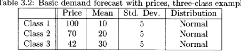
4-5 Demand vector (dk) and partial sum vector (Sk) generation - quantitative example based on Table 3.2... . . . . . . . . 54

4-6 Plot of the partial sums S1, S2 and the resulting Monte Carlo estimates of optimal protection levels for 25 simulated data points... . . . . . . . 55

4-7 Spacenet RM implementation structure . . . ... 57

5-1 Winnebagos and Jeeps mobile outpost exploration concept . . . . 61

5-2 Normalized MEVs versus mission duration using EMEV algorithm . . . . 63

5-3 Normalized MEVs versus mission duration using Greedy-Bid Price algorithm . . . . 63

5-4 Evolution of MEV versus K-factor as a fraction of the deterministic case estimate . 64 5-5 Mission-by-mission capacity allocations for Winnebagos and Jeeps mobile outpost scenario using the EMEV algorithm . . . . 66

5-6 Mission-by-mission capacity allocations for Winnebagos and Jeeps mobile outpost scenario using the Greedy Bid-Price algorithm . . . . 66

A-i An Earth-Moon time expanded network . . . . 72

List of Tables

2.1 Resource Models and Classes of Supply . . . . 30

3.1 Basic demand forecast with prices, two-class example . . . . 40

3.2 Basic demand forecast with prices, three-class example . . . . 44

5.1 Winnebagos and Jeeps mobile outpost exploration detailed plan... . . . . ... 60

Nomenclature

C maximum allocable amount of a resource bj booking limit for class

j

yj protection level for class

j

V(x) optimal expected revenue given unused resource amount x AV Delta-V

CoS Class of Supply

CEV Crew Exploration Vehicle (Orion) CTB Cargo Transfer Bag

CWC Crew Water Container DRM Design Reference Mission EC Exploration Capability

EMEV Expected Marginal Exploration Value EMSR Expected Marginal Seat Revenue ESAS Exploration Systems Architecture Study EV Exploration Value

EVA Extra-vehicular Activity FM Forecasting Module

ISCMLA Interplanetary Supply Chain Management

ISCMLA Interplanetary Supply Chain Management and Logistics Architectures ISS International Space Station

IVA Intra-vehicular Activity LEO Low Earth Orbit LEO Low Lunar Orbit

LL-D Lunar Lander - Descent Stage MBTF Mean Time Between Failure MEC Marginal Exploration Capability MEV Marginal Exploration Value MOE Measure of Effectiveness ORU Orbital Replacement Unit PLM Pressurized Logistics Module REC Relative Exploration Capability REV Relative Exploration Value RM Revenue Management RPM Resource Pricing Module

SHOSS SPACEHAB Oceaneering Space Systems SRU Shop Replacement Unit

TEN Time Expanded Network TPM Technical Performance Measure

Chapter 1

Introduction

1.1

Motivation

Few things capture the imagination as does the exploration of space. However, space exploration is inherently expensive and complex and thus missions are infrequent. There is a huge opportunity cost associated with each and every kilogram of mass launched into orbit and it is critical to maximize the value derived from each and every mission. This paper discusses the extension of the Interplanetary Supply Chain Management and Logistics Architectures (ISCMLA) framework to include the use of revenue management (RM), which is the optimization of the revenue or benefit earned from a fixed, perishable resource [1], in the design, modification, and evaluation of space logistics architectures.

1.2

Space Exploration and Logistics

The next generation of human space exploration will be about true exploration rather than visitation. The focus is on developing the ability to sustain long-term human human presence while reaching deeper into space than ever before. Space logistics, or the movement, storage, and tracking of all crew and equipment necessary to carry out an exploration mission or campaign [2], aims to tackle the challenge of supporting true exploration. It encompasses nearly every aspect of space flight operations with the exception of vehicle and infrastructure design. The ultimate goal is to maximize exploration potential given vehicle performance and infrastructure capabilities, a process which involves answering two key questions:

1. How best to ship cargo and supplies given an exploration architecture? 2. What cargo and supplies should be shipped for a given mission profile?

1.2.1

Mission Types

Unmanned Cargo

Unmanned cargo missions, as the name suggests, are missions conducted with uncrewed vehicles for the purpose of transporting necessary cargo from Earth to in-space exploration sites. Usually unmanned cargo missions are used to deliver large infrastructure items such as habitats and power equipment; they are also used to resupply logistics in support of crewed missions. Unmanned cargo

flights are particularly important at the beginning of exploration campaigns where their large cargo capability is critical in quickly establishing a presence at a site, including an initial inventory. The International Space Station (ISS) relies on unmanned missions carried out by the Russian Progress vehicle to help meet logistical needs [3].

Sortie

A sortie is a stand-alone mission of a relatively short duration (typically 2 weeks or less) that allows the exploration of a site without the need to preposition habitats, infrastructure, and consumables. Sortie missions also allow for exploration of high-interest science sites or scouting of future lunar outpost locations. In sorties, crew members typically live in the vehicle they travel in, and have limited mobility around the site. The crew has the capability to perform daily EVAs (extravehicular activity), typically with all crew members involved to maximize the scientific and operational value of the mission. All of the Apollo missions and most of the Space Shuttle missions have been sortie-style missions.

Outpost

Outpost missions are a series of extended flights to the same location. The longer duration (typically 1-6 months per flight) means that outpost missions usually involve significantly more infrastructure than sorties. The crew usually has a dedicated habitat separate from the transportation vehicle, which in turn drives the need for more advanced power generation, in-situ resource utilization, and cargo storage infrastructure. Outpost missions also tend to include more advanced surface mobility infrastructure to allow for expansive exploration, rather than being limited to the immediate area around the outpost site. While surface operations during sortie missions are typically dominated by EVAs, outposts typically feature a more balanced schedule of EVA and IVA (intravehicular activity) due to limitations from the extreme radiation environment in space, the fatiguing nature of EVA op-erations, space suit maintenance and repair, and portable life support system logistics [4]. Outposts are not limited to surface locations, but can also include in space sites. The International Space Station (ISS) is an outpost in low earth orbit, and outpost missions to ISS are called "expeditions".

Mobile Outpost Concept

The mobile outpost is a hybrid of the sortie and outpost mission types. Mobile outposts combine some of the best aspects of the sortie and outpost mission types by providing the operational flex-ibility to explore multiple sites while maintaining more infrastructure in service between missions, thereby increasing exploration capability at each site. However, mobile outposts depend first and foremost on efficient, lightweight mobility systems, and also on highly capable power systems inte-grated into each lander, large habitat shells that can double as pressurized logistics modules (PLMs), and simplified mating (access, fluids and electronics) of habitat and/or logistics modules. In other words, mobility adds technological and development complexity to an exploration program. To date, no space exploration campaign has relied on the mobile outpost concept, however the increasing ca-pability of mobility platforms like NASA's ATHLETE have brought mobile outposts to the forefront (see Appendix C).

1.2.2

Logistics Strategies

There are several different logistics methodologies which combine with the various mission types to form an exploration architecture. The ISCMLA framework defines four different classifications of logistics methodologies based on the study of terrestrial supply chains:

Pre-positioning This approach focuses on sending cargo and supplies to the exploration site ahead of the crew, or more generally when the demand materializes [5]. It is typically achieved through the use of unmanned cargo flights early in a campaign that deliver supplies and infrastructure in bulk. However, pre-positioning can also be achieved by using excess cargo capacity on manned flights to build up a gradual stock of supplies.

Carry-along In this approach, all cargo needed for a given mission is brought along on that mission; in essence each mission is self-contained, and its duration and scope is limited by the cargo-carrying capability of the vehicles used for that mission.

Resupply In this approach, some cargo is carried along by the crew, but is then supplemented by scheduled and/or need-based resupply flights. Scheduled resupply flights are pre-determined cargo deliveries to meet predicted demands (based on historical demand models). In practice, need-based resupply flights are difficult to achieve due to the long lead time required for launch preparation.

Depot This approach involves the use of an intermediate distribution center somewhere between the origin and destination of cargo items. The depot methodology stems from the terrestrial concept of a multi-echelon supply chain where inventory is held in a depot until it is demanded by the retailers or customers.

Conceptually, mission types and logistic methodologies are decoupled. However, in practice, certain logistics methodologies work much better with certain mission types. For example, although it is possible to have a "super sortie" in which an unmanned cargo flight supports a future crewed flight, sorties almost always employ a carry along strategy. As exploration architectures become more advanced, they are supported by increasingly advanced interplanetary supply chains utilizing more advanced logistics methodologies. In many cases, these methodologies will be hybrids of the methodologies described above. Figure 1-1 shows a simulated logistics strategy for the Constellation lunar architecture, which also uses a mix of carry-along and pre-positioning [6].

1.2.3

The ISCMLA Framework

The ISCMLA project aims to study human space exploration from the logistics perspective. As a result, the modeling framework is quite different from those of traditional space exploration studies. It focuses primarily on the flow of crew and materials through time and space, with compact para-metric representations of vehicle form and function. The following terms are commonly referred to in the Interplanetary Supply Chain Management and Logistics Architectures (ISCMLA) framework, which includes the following concepts:

Classes of Supply (CoS) capture the main functional categories of cargo that are needed to sup-port human exploration. Figure 1-2 shows the ten primary classes, which are further divided into forty-four sub-classes and are used for demand estimation and manifesting of individual missions. This detailed CoS definition enables fine-grained modeling of material flows that

enables analysts to determine not only if enough supplies are at a given site, but also that there are the right types of supplies at the right time.

Resources are the basic unit the producer uses to generate exploration value

Networks are graphs of nodes and edges (i.e. locations and transportation links) that define and connect all points of interest. Networks are also traditionally used in terrestrial transportation systems to represent physical locations and the transportation links of various modes between them. For space transportation networks, the concept of a location is abstracted to represent points of interest, such as orbits or Lagrange points. Note that transportation links in space are generally time-varying due to astrodynamical motion (see Section 2.1.1).

Processes are the building blocks of scenarios

1.

Measure of Effectiveness (MOEs) quantitatively evaluate specific space exploration scenarios and interplanetary supply chains. Note that MOEs are only proxy metrics for comparative purposes, not for absolute forecasting.

Technical Performance Measures (TPMs) are feedback metrics that inform the user about infrastructure performance, resource utilization, and safety margins.

1.3

Revenue Management

Revenue management (RM) deals with the maximization of the revenue or benefit earned from a fixed, perishable resource in uncertain conditions [1]. While revenue management as a formal practice has its foundations in the airline industry, it has spread in the last two decades to cargo services, hotels, car rental companies, and e-commerce. These industries, particularly airlines and cargo services, have many features that are analogous to those of space exploration. However, at the time of writing, to the author's best knowledge RM has not been used in space logistics. The goal of this thesis is to explore the applicability of RM to space logistics, and the following sections present the space analogy in more detail.

1.3.1

Requirements and Characteristic Features

The basic revenue management problem requires four entities: customers, producers, resources, and revenue. Customers seek to attain some perishable resource, which are units of capacity managed by the producer. Each customer has a price they are willing to pay for that resource. The producer controls the allocation of the resource and therefore "produces" resource bundles that are offered to customers. The challenge for the producer is to sell the right resource(s) to the right customer at the right time in order to maximize revenue.

Most transactional business models are candidates for revenue management at some level. How-ever, only in certain types of these businesses do the costs and complexity of implementing a revenue management system outweigh the benefits. Muller defines four characteristics that make a particu-larly good revenue management problem [7]. These are:

'A scenario is the full specification of the logistical aspects the user wishes to model (see Section 2.1 for more

EPre-positioning * Carry Along

- r

~

1 2 3 4 5 6 7 8 9 10 11 12 13

Flight Number

14 15 16 17 18 19 20 21

Figure 1-1: Simulated logistics strategy for nominal Constellation campaign. The strategy shown uses a combination of pre-positioning and carry-along to maintain mission robustness through safety stocks (pre-positioning) while allowing for flexibility to adapt mission profiles (carry-along).

Figure 1-2: Functional classes of supply for human space exploration.

100% 90% 80% 70% 60% 50% 40% 30% 20% 10% 0% ... .... ... .... .... ... ... .... ... r.. .: ... ...

1. Customer Heterogeneity: customers place different values on resource units. The possibil-ity of segmenting price-sensitive customers is key in implementing revenue management. The most common mechanism used to segment customers is the time of purchase; that is, the less price-sensitive customer generally purchases nearer the time of production.

2. Demand Uncertainty: demand is stochastic, difficult to predict, and cannot be satisfied using existing stocks.

3. Limited operational flexibility: resource units are limited and there is a consistent mis-match between the supply and demand. Additionally, the means to balance supply and demand are limited.

4. Standardized Product Range: the nature of resources on offer remains essentially unaltered over a substantial period of time. This is key to being able to predict future demand.

In other words, A good revenue management candidate industry sells products that are perishable, faces time-varying demand, and is burdened with large fixed costs while variable costs are small in the short run. Due to the low marginal cost and high fixed cost condition, increased revenue essentially translates directly to increased profits.

1.3.2

Industry Examples

The airline industry is the prototypical example of the characteristics defined in Section 1.3.1. First, airlines certainly experience customer heterogeneity; business travelers, vacation-goers, students, a host of other groups each have different valuations of the same resource (a seat on the plane). Second, the airlines cannot satisfy demands using existing stocks. It is impossible to consistently satisfy demand for a Friday evening flight from Seattle to Boston with seats on Thursday morning flight. Third, aircraft are large, blocky, and expensive capital investments that have a very finite capacity. It is prohibitively difficult and expensive for airlines to expand or contract their supply in the short or even medium term; they cannot simply make more products (seats) to sell to meet demand. Finally, seats on an aircraft are an extremely standardized product, even across competitors. And the same product is offered whether demanded 30 days or 30 minutes before production (departure). The initial success of Revenue Management in the airline industry drove an expansion first into the hotel and rental car industries, and then further into cargo shipping, restaurants, and a whole host of other industries. Depending on the needs of the industry, revenue management is used to increase resource utilization (sell more products), segment customers through packaging resources, adjust demand profiles, and/or dynamically price resources.

The following provides a brief overview of how revenue management is used in some key industries: Hotels use RM techniques to provide special rate packages for periods of low occupancy. They also use overbooking policies (refer to Section 3.2.3) to compensate for cancellations and no-shows. Restaurants use RM to even out demand over the course of the day. They offer discount coupons or charge reservation fees and higher meal prices during peak periods in order to move customers to off-peak periods.

Attractions (e.g. theme parks and carnivals) set different admission charge levels, provide joint-entry tickets, group discounts, coupons, membership rates.

Rental car companies use RM-based controls to vary prices frequently according to demand, and to accept or reject booking requests. A big driver in this industry is the balance of weekend demand from vacationers and weekday demand from business travelers.

Cargo and freight companies use RM to determine the price of a shipment based on space re-quired, location and comfort. They also use RM to determine the optimal ship size and capacity for each shipment class (e.g. overnight, 2nd day, and ground).

IT Services use RM to allocate administrator time, computing capacity, storage, and network capacity among segments of customers and determine an appropriate price for each segment. Sections 3.1.2- 3.1.5 present an overview of the unique aspects of RM problems in each of the above industries and related research.

1.4

Space Exploration and Revenue Management

Typically, the logistics strategies are developed in response to mission profiles. Within the logistics strategy, cargo is delivered to meet pre-defined availability targets. The use of RM in this process allows this question to be approached from a different perspective. Like in the airline and cargo examples, in space logistics revenue management can be used to allocate cargo delivery capacity (i.e. cargo mass and volume) in order to maximize productive exploration given uncertainty in demand. This in turn defines the availability targets, which helps to define the logistics strategy. Combined with the existing forward approach, this reverse approach allows a bi-directional approach to the design of logistics strategies. When paired with the SpaceNet simulation framework, to be discussed in Chapter 2, revenue management may have the following potential applications:

* Development of design reference missions (DRMs), particularly for exploration architectures that rely on extended sorties or mobile outposts.

" Refining mission profiles in response to vehicle performance and demand uncertainty. " Optimal manifesting of spacecraft in the operational phase of missions.

1.4.1

Suitability for Revenue Management

In the airline case, for example, it is fairly straightforward to identify the customers, producers, resources, and revenue. The customers are passengers, the producers are the airlines, the resources are the seats, and the revenue is money. The space exploration example is perhaps more subtle than the airline example, but nonetheless it has both the requirements and characteristic features to be a strong candidate for the implementation of revenue management. There are essentially there are two types of customers: 1) the exploration agents2, and 2) the surface infrastructure at the exploration site. The producers are the various agencies conducting exploration, e.g. NASA or ESA, which must manage their resources in order to maximize their utility from exploration. The resource is the combined mass and volume available for cargo on spacecraft heading to the exploration site; this can be broken down into a pressurized and unpressurized component. Finally, the revenue is the the contribution of the item consuming the resource to productive exploration.

Not only does space exploration have the major entities for the implementation of revenue man-agement, it also shares the characteristic features. These are:

2

" Heterogenous Customers: Exploration agents (generally crew, but sometimes robotic sys-tems) generate demands for provisions and operational equipment. Surface infrastructure are those elements needed to support the exploration agents. These include habitats, power units, and mobility systems and their demand is primarily in terms of spares. These customers demand different amounts of the resource and "pay" different amounts for the resource. * Demand uncertainty: Demand for crew provisions is relatively deterministic on average,

particularly for longer missions. In contrast, demand for spares is extremely uncertain due to limited production quantities for flight hardware, relatively immature designs (compared to most Earth-bound complex systems), and environmental factors.

" Limited Operational Flexibility: Space flights are infrequent, typically scheduled far in advance, and face very tight mass margins. There is very limited ability to change supply to meet demand.

* Standardized Product Range: the contribution of the bundle of manifested resource to productive exploration. Ultimately exploration agencies are in the business of maximizing their benefits from exploration.

1.4.2

Challenges

One major challenge in the implementation of RM in space logistics is the definition of revenue. Ultimately exploration agencies are in the business of maximizing their benefits from exploration, as complex as those may be to define or quantify. Benefits can be in the form of scientific discovery, resource discovery, operational knowledge, and/or political gain.

A related challenge is that the revenue is not earned at the time of "sale". Generally speaking, the revenue earned from a customer is not known when a spacecraft is launched, or even when it arrives at the exploration site. Rather revenue is generated on the back end when the item is actually used in the mission. Thus the decision for the producer in this problem is not only one of ensuring that resources are sold to the most high-revenue customers, but also whether or not each customer will actually pay for the resource within a given time horizon.

1.5

Thesis Organization

This thesis consists of six chapters, as shown in Figure 1-3. These are:

Chapter 2 gives an introduction to SpaceNet, an integrated modeling and simulation tool. SpaceNet, co-developed by MIT and JPL, allows the user to explore the various logistics strategies dis-cussed Chapter 1. In particular this chapter talks about SpaceNet 2.0, the 2nd generation of the software, which has added flexibility and capability to support more advanced logistical concepts.

Chapter 3 presents foundational revenue management concepts including price-based and quantity-based revenue management. It also provides an overview of various formulations and solution approaches.

Chapter 4 presents the main contribution, the SpaceNet Revenue Management module (SpaceNet RM), which is capable of optimizing campaign exploration performance under uncertainty. This chapter also introduces a space logistics-based definition of revenue.

Chapter 5 presents two case studies where revenue management was applied to help evaluate proposed campaigns.

Chapter 6 outlines several future directions for SpaceNet RM. It concludes with a summary of contributions.

SpaceNet RM Software

Chapter 5:- Case Studies

Results

FChapter 6: Conclusions &

jauture}VWork- e

Chapter 2

SpaceNet 2.0: Integrated Modeling

and Simulation

The goal of SpaceNet is to allow a user to model and evaluate an exploration mission as an inter-planetary supply chain with the purpose of answering key logistics questions [8]. These answers provide insight into the bottlenecks in the transportation architecture, strategies to maximize ex-ploration capability, and the impact of uncertainty on logistics strategies. SpaceNet models and simulates processes, element instantiations, and supply item levels, and other logistical aspects of a campaign in a high fidelity, enabling it to respond to complex issues such as campaign robustness

and contingency analysis while providing an end-to-end analysis capability.

2.1

Scenario Building

A scenario is the full specification of the logistical aspects the user wishes to model. It essentially defines the who, what, when, where, and how of all material flows while appropriately abstracting the how of the technologies that enable space exploration. Building a scenario involves 5 basic steps:

1. Defining a network

2. Defining the mission (i.e. the various exploration and transportation processes) 3. Defining resource models

4. Manifesting supply items (i.e. implementing a logistics strategy) 5. Processing simulation feedback

The following sections provide an overview of each of these steps, and upgrades and added features in SpaceNet 2.0, which is the most recent version of SpaceNet developed at the time of writing. The upgrades to be discussed are designed to allow more flexible modeling, greater interoperability with other tools and models, and to support the implementation of revenue management in SpaceNet.

2.1.1

Defining the Network

Unlike most terrestrial networks, space networks have time varying properties; a path that may be available at one time and may be unavailable at another. SpaceNet addresses these properties

by defining two types of networks. First, there is the static network which represents the set of physical locations (i.e. nodes) and the possible connections between them (i.e. arcs). Second, there is the time-expanded network (TEN) which adds the dimension of time to the static network to enable dynamic behavior, while abstracting the details of orbital mechanics. The time-expanded network has the ability to capture the time-dependency of interplanetary trajectories, including launch windows and tradeoffs between fuel consumption and time-of-flight. Appendix A provides some additional detail about both types of networks and their representation.

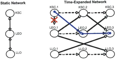
Static Network Time-Expanded Network

KSC,1 KSC,2 KSC,3

KSC

LEO,1 LEO,2 EO,3

LEO

LLO

Figure 2-1: Left: Static network including NASA Kennedy Space Center (KSC), Low Earth Orbit (LEO), and Low Lunar Orbit (LLO). Right: the corresponding time expanded network. In this network, one can see that moving from KSC to LEO requires one time step. Therefore it is impossible to move from KSC,1 to LEO,1 while it is possible to move from KSC,1 to LEO,2. It is however, always possible to stay at a node, and therefore a movement from LEO,2 to LEO,3 is allowed.

To build a network, the user first defines the static network explicitly by adding desired nodes. As a user adds and removes nodes, arcs are automatically added and removed accordingly to show the possible paths throughout the static network in real time. The time expanded network is automatically generated from the user constructed static network based on a chosen time step At. Of course, time expanded networks can grow to be very large depending on the size of the static network and/or the length of the scenario. For example, a time expanded network for a 3-year scenario (about 1000 days) with 10 nodes and a time step of 0.1 days (Earth days) and will have more than 100,000 nodes. This is an issue both in terms of the users ability to manage all the information, and from a computational resource management perspective. To address both issues, the user interacts with the TEN through processes, which identify which parts of the TEN experience logistical activity. Processes, discussed in Section 2.1.2, enable the generation of a "sparse" time expanded network, which address both ease of use and resource management.

SpaceNet 2.0 also features a shortest path algorithm that can assist the user in finding the shortest path between two nodes (if any exists) based on minimizing either cumulativeAV, duration, or number of orbital transfers (i.e. arcs). The algorithm uses an A* search to look through a database of stored trajectories and returns a pathway, or series of connected arcs to the user. If the pathway contains nodes not in the network at the time of search, the software gives the user the option to add them into the network.

-2.1.2

Defining the Mission

As briefly discussed in the previous section, processes define the movement of elements and cargo throughout the time expanded network. They define the how and when in the supply chain. The ISCMLA framework defines five core processes [2]. These are:

Exploration processes model exploration and science activity at a specified node. This is typically a surface node, however exploration can also happen at in-space nodes (e.g. in the ISS). Proximity Operation processes model local rendezvous/docking, undocking/separation, and

trans-position of elements.

Transfer processes model the transfer of agents and/or supply items. In orbit, transfers must be from one element into a different co-located element. On the surface, transfers can also be between an element and a node, for example a sample return to earth.

Transport processes model the relocation an element to a new physical node along an allowable arc.

Waiting processes model remaining at the same physical node for some number of time periods. In a given process, the user can dynamically create instantiations of elements from a collection of templates, which are derived from elements used in past and future exploration campaigns such as ISS and Constellation. Alternatively, the user can select from previously instantiated elements and continue using them throughout a scenario. Previously instantiated elements can include the propulsive stages and surface systems delivered to an orbit by a launch vehicle. These elements may be be used in future processes until they reach a surface location. Processes can be grouped into composite processes, which provide a layer of abstraction to simplify scenario building. Typically a composite process encompasses the constituent processes of a sortie, unmanned cargo flight, outpost flight, etc.

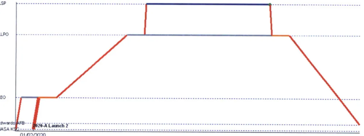
LEO ---- - - -- - - - ---

---...--- ---...---...--- ---...---...--- ---...---...--- ---...---...--- ---...---...--- ---...---

---Edas 2-A Launch?2~-

---NASKO -- ---...

---01 A22020

Figure 2-2: Space logistics processes. The horizontal axis represents time, while the vertical axis represents node location. Blue = Exploration, Orange = Proximity Operation, Green = Transfer, Red = Transport, Gray = Waiting.

2.1.3

Defining Resource Models

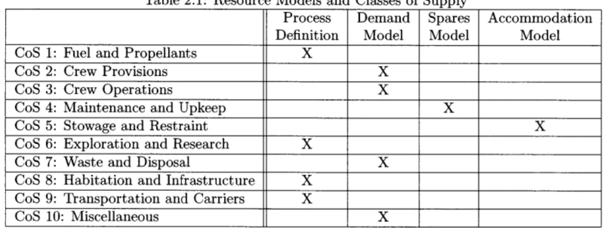
Generally, demands for habitation and infrastructure (CoS 8) and transportation and carriers (CoS 9) are defined explicitly as part of the scenario building process. Likewise, demand for fuel and propellants is a result of the definition of demand for CoS 8 and CoS 9 and the process definition. However, demand for the remaining classes of supply is typically complex and dependent on the details of the exploration architecture and must therefore be specified by the user. SpaceNet 2.0 captures these demands through 3 resource models: The demand model, the spares model, and the accommodation model.

Table 2.1: Resource Models and Classes of Supply

Process Demand Spares Accommodation Definition Model Model Model CoS 1: Fuel and Propellants X

CoS 2: Crew Provisions X

CoS 3: Crew Operations X

CoS 4: Maintenance and Upkeep X

CoS 5: Stowage and Restraint X

CoS 6: Exploration and Research X

CoS 7: Waste and Disposal X CoS 8: Habitation and Infrastructure X

CoS 9: Transportation and Carriers X

CoS 10: Miscellaneous X

Demand Model

The SpaceNet 2.0 demand model is a tree-based data structure that allows the user to define arbitrary demand structures for crew provisions (CoS 2), crew operations (CoS 3), and waste and disposal (CoS 7). A demand model is an aggregate of demand variables, of which there are two types: rate variables and reference variables. Rate variables define demand for a particular supply item, a consumption rate, and a unit of measure. Users may select from a variety of parametric probability distributions or use a deterministic value for the rate. Reference variables define demand for a particular supply item in terms of fractions of another supply item. For example, the leakage rate of oxygen and nitrogen in a habitat can be represented as a reference variable that is referenced to the habitat volume.

Spares Model

The spares model is used to define the demand for spares and related equipment for infrastructure (i.e. elements) specified in the scenario building process. The spares model can be specified in two ways, which are spare-by-mass and spare-to-availability.

The spare-by-mass calculates the mass and volume of pressurized and unpressurized spares for a given time period for an element as a function of its dry mass. Spare-to-availability calculates spares demands as a function of element orbital replacement units (ORUs) and shop replacement units (SRUs). Such demands are application-specific and rely on attributes such as mean-time-between-failure (MTBF) and duty cycle. Specifically, sparing by availability calculates a "buylist" of spares needed to meet a desired target availability specified by the user (the default value is 95%). The total mass and volume of spares required is then obtained by multiplying the quantity of each ORU in the

buylist by its mass or volume respectively. SpaceNet returns a buylist that meets the availability target even if it violates the resource constraint (i.e. the amount of cargo mass and/or volume available for delivering spares to the exploration site). In this case, SpaceNet also gives the user the option to recalculate the spares based on the highest estimated availability that is achievable.

While sparing-to-availability is more accurate than sparing-by-mass, it cannot be used until the element ORUs and SRUs are well-defined, which makes it difficult to use in immature exploration architectures where that information is not well known. The spare-by-mass functionality provides a reasonable approximation for spares demands as a temporary measure while an architecture mature and reliable data becomes available.

Accommodation Model

The accommodation model captures the demand for stowage and restraint (CoS 5) based on the results of the demand model. Users have the option of specifying an arbitrary number of accommo-dation mappings, each of which pairs a supply item type with a particular packing container type, and sets a packing efficiency for the container type which essentially indicates when to stop mani-festing a container and start manimani-festing a new one. There may be multiple mappings per supply item. For example, food-related supply items might be paired with cargo transfer bags (CTBs) and spares items with SHOSS boxes; water may be paired with a full-size water tank as well as with a smaller crew water container (CWC). SpaceNet 2.0 selects the best containers for each demand based on minimizing the tare fraction and maximizing container capacity utilization. Containers are manifested based on maintaining a clear separation between supply classes and consumers (i.e. elements and agents), for example an individual container may be packed with food and related items for the CEV, but may not be packed with a mix of food and waste disposal equipment for the CEV and LL-D, respectively. This reflects typical real-life manifesting practice.

2.1.4

Forecasting Demand

The Forecasting Module (FM) is a basic implementation of the full discrete event simulator that utilizes the demand model to estimate scenario demands based on a target availability. The FM flattens the demand model, parses demand units, and performs the necessary mathematical opera-tions are performed to produce a demand in terms of physical units of weight and volume. The FM has two modes: standard mode and quick estimation mode.

In standard mode the FM receives an event schedule for the simulator corresponding to the desired forecasting horizon. From this point the FM can proceed either deterministically or stochas-tically. For deterministic estimation, the FM estimates demand by event according to the nominal (mean) value of each demand variable. For stochastic estimation, the FM uses inverse transform sampling, which allows the generation of samples of arbitrary probability distributions [9], to pro-duce an estimate of the demand value for each event. The SpaceNet 2.0 forecasting module currently supports uniform, normal, lognormal, triangular, exponential, Weibull, and Poisson distributions.

Once demands are estimated for each event, either deterministically or stochastically, the FM merges demand by consumer, i.e. the entity that generated the request for resources. If the event schedule spans multiple process groups, demands for each element are further merged by process group. Finally, the forecasting module can optionally pack raw demands into containers based on the accommodation model. Users can also specify a global tare fraction, in which case the FM packs demands into a generic container with the appropriate specifications.

2.1.5

Manifesting Demand

Calculating the demand determines the nominal amount of cargo required to support the surface systems and exploration agents in a campaign. To understand if such a campaign is feasible, and to evaluate what the most effective delivery strategies are, the packed items must be manifested into cargo carriers. Manifesting the discretized supply items into cargo carriers must satisfy multiple constraints. The cargo carrier must have the available pressurized or unpressurized mass and volume capacity for a given supply item. If the cargo carrier, such as a pressurized logistics module (PLM), is nested in another element such as a descent stage, then the cargo capacity of that parent element must be satisfied as well. In addition to the supply items created by the cargo demands from the surface systems and exploration agents, a user can also manifest exploration items such as science instruments, and reserve supplies such as safety stocks. These reserves would serve to hedge against uncertainties in demand or flights that are delayed or cancelled. While the manifesting process can be performed by hand to optimize packing efficiency, it can also be completely automated using a pair of simple heuristics.

2.2

Simulation

Simulation ties together all other components of the modeling framework, taking the mission scenario as an input and producing the output information that evaluates both the feasibility and effectiveness of the scenario.

2.2.1

Discrete Events

SpaceNet is built on discrete event simulation, whose strength lies in the ability to model random events and to predict the effects of the complex interactions between these events. This flexibility allows various hypotheticals to be investigated by changing inputs to the model and then comparing the outcomes. This makes discrete event simulation a strong decision support tool.

In logistics, the important pieces of information for the user are the states of simulation entities before a given process occurs, the characteristics of the process, and the entity states after the process is completed. For instance, if an element is placed in LEO and then transported to the lunar surface, the key pieces of information are the states of the element and node before the transportation process (mass and crew/cargo of the element, physical node characteristics and time), characteristics of the transportation process (e.g. the departure node, AV, time of flight, and arrival node), and information after transportation process (e.g. residual propellant) Thus the space logistics framework is more suited to an event-driven approach than to a time-driven approach.

SpaceNet 2.0, unlike previous versions, redefines the 5 core processes as composites of events, which are the new atomic unit of simulation. The following subsections discuss the modeling and performance advantages of using events as the atomic unit of simulation. At the time of writing the set of events includes:

" Arrival events model the arrival of an exploration resource to a node.

" Departure events model the departure of an exploration resource from a node.

" Explore events model exploration activity such as EVAs and performing of experiments. Typically an Explore event represents a single EVA.

" Burn events model the firing of main engines and/or reaction control systems in a single element.

* Stage events model the staging (i.e. detachment from an active stack for discard) of an element, usually during a transport process, but occasionally during a wait or proximity op-erations process.

" Relocate events model the movement of scenario entities from one node to another. This includes surface relocations as well as orbital relocations. Relocation events are composites of arrival and departure events, but include a duration for generating rate-based demands. " Transfer events model the movement of supply items from one container to another container,

where a container is any element or supply item that can hold supply items, and all surface nodes.

Based on the manner in which events are generated, processes can be simulated in more or less detail based on simulator performance or user preference. For instance a user may choose to increase precision for Exploration processes while reducing precision on Transport processes. This enables the user to make better tradeoffs in terms of speed and precision and change his or her preferences in different parts of the same simulation. In addition to enabling variable precision simulation, events also enable custom processes. Exposing some events to the users allows users to design custom processes by combining events as desired. This is particularly important for surface operations which require detailed specification to model accurately.

2.2.2

Clock Management

SpaceNet 2.0 introduces a next-event time advance approach, which is the most common approach used in major simulation packages [9]. In contrast, previous versions of SpaceNet used a time step approach. With a next-event time advance approach, the simulation clock is advanced to the next scheduled future event, which is then executed. The system state is then updated and the system clock moves to the new next scheduled future event as shown in Figure 2-3. Concurrent events are made sequential by giving execution preference to the event originating from the earliest initiated process.

The advantage of the next-event time advance approach are reduced simulation time since only time periods with events are analyzed, and also accuracy since events are always executed on time and in sequence (rather than as part of a batch). This improvement in speed and accuracy allows SpaceNet 2.0 to perform simulation runs in the background, providing the user with various pieces of useful data, while supporting implementation of Monte Carlo simulation.

2.2.3

System State and Histories

During simulation, each agent, supply item, element, and node is tracked and its history recorded. These histories are used for calculating performance measures, visualization, and user post-processing of simulation data. The 3 types of history are:

EHistory tracks the elements, giving the location and transportation history of each element. It also provides the mass (propellant and dry mass) and crew/cargo information for each element.

NHistory tracks the nodes and provides information on which elements are located on each node at a specific time.

CHistory tracks crew/cargo and shows which element the crew/cargo belongs to at a specific time.

The three histories have built-in redundancy and form different interpretations of the same mission scenario. Together, the three combine to provide a complete reconstruction of each simulation run. For instance, NHistory, EHistory, and CHistory combine to provide a complete record of the supply levels of each supply class at a given node. SpaceNet 2.0 is capable of outputting each history in Excel and XML formats.

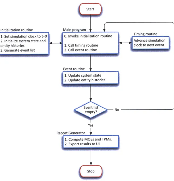
Sta rt

Initialization routine Main program I

1. Set simulation clock to t=0 0. Invoke initialization routine Timing routine

2. Initialize system state and Advance simulation

entity histories 1. Call timing routine clock to next event

3. Generate event list 2. Call event routine

Event routine

1. Update system state 2. Update entity histories

Event list _No empty?

Yes Report Generator

1. Compute MOEs and TPMs. 2. Export results to UI

Figure 2-3: SpaceNet 2.0 variable time advance clock management

2.2.4 Performance Measures

An important final step in supply chain design and analysis is the ability to process the simulation output in such a way that architectures can be evaluated and compared [5]. Several metrics (termed measures of effectiveness or MOEs), have been developed hand-in-hand with the simulation and modeling framework to enable the comparative evaluation of logistics architectures [2]. MOEs pro-vide a quantitative way to evaluate specific space exploration scenarios and interplanetary supply chains in general. It is important to note that MOEs are proxy metrics for comparative purposes, not for absolute forecasting. MOEs continue to evolve to better capture new exploration paradigms and the benefits derived from unmanned activities such as the presence of robots on planetary surfaces and orbiting spacecraft observation. MOEs fall into three broad categories:

Basic Logistics Performance: Any mission's performance is largely defined by the capability of the launch vehicles and space craft involved, as well as their utilization. The basic logistics performance MOEs are designed to quantitatively measure capability and utilization, thereby providing the user an performance envelope within which to modify and optimize the distri-bution of mass between supply classes as desired.

Exploration Capability: The true benefit (revenue) of planetary space exploration is not mone-tary, but comes primarily from healthy and qualified explorers, scientists, and robotic systems (i.e. agents) being able to spend a certain amount of time at one or more nodes. To first order, revenue scales linearly with both the number of agents as well as the duration of their stay. In addition, specific exploration equipment, scientific instruments, and surface infrastruc-ture items play a large part in facilitating exploration, and act as multipliers for exploration productivity. The exploration capability MOEs are designed to capture this concept.

Relative Cost and Risk: To first order the cost of a scenario scales with duration (operating and observation costs) and launched mass (development and recurring costs). The actual details of both risk and cost however are extremely complex and beyond the scope of the logistics modeling framework. Thus the the Risk and Cost MoEs relate risk and cost in these relative terms without attempting to define a precise probability distribution for risk and/or an absolute monetary value for cost.

Appendix A provides detailed equations of the measures of effectiveness.

2.3

Data Management

In an attempt to improve asset management for human space-flight missions to the Moon and Mars, a relational database for interplanetary exploration, aptly named the Interplanetary Supply Chain Management (ISCM) database has been developed. This database incorporates inventory management capabilities with extensive capabilities for manifesting, spares requirements planning and mission planning. Information maintained in the integrated database includes astrodynamics data, element data, commodities data, and spares data. SpaceNet uses an enhanced version of the ISCM database to store all the information required by the model, as well as to store in-process data as the user designs a scenario.

2.4

Chapter Summary

This chapter has described an interplanetary logistics modeling and simulation tool, SpaceNet 2.0, developed by systems engineers at JPL and MIT. The goal of SpaceNet is to allow mission architects, planners, systems engineers and logisticians to focus on what will be needed to support future crewed exploration missions, primarily in the Earth-Moon-Mars system. Instead of helping to design the elements (vehicles) themselves in terms of propulsive and pressurized/unpressurized cargo carrying capability, SpaceNet evaluates such vehicles in the context of a particular mission architecture and supply chain strategy. The emphasis is on ensuring the logistical feasibility of a given scenario as well as a prediction of the resulting logistics measures of effectiveness (MOEs). All this is enabled by detailed simulation of time-varying flow of elements, crew and supply items through the nodes and arcs (trajectories) of a supply network in space, taking into account feasibility (AVs, fuel levels) as well as consumption and supply.