Capabilities and limitations of Phase Contrast Imaging techniques with X-rays and neutrons

(1)

CAPABILITIES AND LIMITATIONS OF PHASE CONTRAST IMAGING TECHNIQUES WITH X-RAYS AND NEUTRONS

ANTONIO LEONARDO DAMATO B.S., M.S., Engineering Physics (2001)

Politecnico di Milano, Milan, Italy Ecole Centrale Paris, Paris, France

MASSACHUSEfTT INSTITUTE OF TECHNOLC'Y

AUG

19 2009

LIBRAR %IES

SUBMITTED TO THE DEPARTMENT OF NUCLEAR SCIENCE AND ENGINEERING IN

PARTIAL FULFILLMENT OF THE REQUIREMENTS FOR THE DEGREE OF DOCTOR OF PHILOSOPHY IN NUCLEAR SCIENCE AND ENGINEERING

AT THE

MASSACHUSETTS INSTITUTE OF TECHNOLOGY

A' Signature of Author: Certified by Certified by_ Accepted by_ Antonio L. Damato 9partment of Nuclear Science and Engineering

, / January 6, 2009

Richard C. Lanza Senior Research Scientist

VThesis

Supervisor

V

Berthold K. P. Horn

Professor of Computer Science and Engineering Thesis Reader

( V Jacquelyn C. Yanch

Professor of Nuclear Science and Engineering Chair, Department Committee on Graduate Students

FEBRUARY 2009

Acknowledgements

First and foremost, I would like to acknowledge Dick Lanza. Dick is an excellent advisor and an excellent scientist, and it has been a pleasure to learn from him and work with him.

This work would not have been possible without the help of my committee members. Professor Berthold Horn was involved in this project from the start and this thesis owes its best contributions to him. Many thanks to Professor Jacquelyn Yanch for the excellent feedback and helpful suggestions.

The students, faculty and staff in the Francis Bitter Magnet Lab were very supportive. My officemate Eric Johnson for helping me with coding and for the useful discussion; Jayna Bell for her patience in letting me schedule my experimental work with "her" X-ray tube, and Gordon Kohse for assisting in the experiments; Professor David Cory and his group for the useful discussions and the help with the experimental equipment; and a special thanks to Rachel Batista, for always being there when I needed her.

The MIT Reactor Laboratory was very supportive. Many thanks to Yakov Ostrovsky for the help in designing the neutron facility, and to Peter Binns for mentoring me through many of those experiments.

Professor John Idoine of Kenyon College was a terrific mentor. Roberto Accorsi of Children's Hospital of Philadelphia is the undisputed expert on Coded Apertures and provided invaluable help in the CSI development.

Finally, I thank my wife, Gretchen DeVries, for her love, encouragement, and support; and my parents for their ongoing support. My newborn daughter, Cristina Silvana Damato, did not have much patience with me writing this thesis, but she certainly provided me with the strongest motivation I could possible find to finish.

(4)

1. Introduction

Non-destructive imaging of a sample is a common analysis technique used for applications as varied as radiography of a broken bone, routine mammography, a CT scan or a PET exam for tumor diagnosis, morphological ultrasound of a fetus, and security scanning of luggage at airports. The use of these imaging techniques is even more widespread than the immediately apparent applications; the same technology is used for scanning of containers at ports for homeland security reasons, neutron and X-ray imaging of the microstructure of mechanical parts such as turbines, and investigation of defects in industrially manufactured products. The list of applications for non-destructive testing is long.

ii

Figure 1: Progress in X-ray imaging. (a) Rontgen's wife hand (1896); (b) Baggage scanner CT (2006); (c) Mammogram (2006).

Of these techniques, the one with which the general public is probably most familiar is X-ray radiography. This technique is based on the ability of X-rays to be only partially absorbed as they travel through materials. Differences in absorption between various parts of a target object allow the imaging and identification of internal structural details of the object. Used for a variety of applications, X-ray radiography has a history of success. X-rays were discovered in 1896 by R6ntgen, who famously took a picture of his wife's hand to demonstrate an early application of X-ray radiography. Subsequent technical advancements enabled X-ray radiography to be used for high quality three

(7)

dimensional imaging, for instance for medical applications and for security screening at airports (see Figure 1).

Not surprisingly, X-ray imaging is generally used to image heavy, dense materials, which are opaque to X-rays, surrounded by soft, less dense materials, which are more transparent. A classical example is the imaging of bones in tissue: the radiation passes through tissue but is absorbed by bones, resulting in an image of the "shadow" of a bone on the X-ray film. The success of X-ray imaging has made it possible to extend the applicability of this technique beyond the relatively straightforward requirement to distinguish soft tissue from bone. For instance, most mammography examinations utilize X-rays; in this case, the goal is to identify cancerous soft tissue surrounded by healthy soft tissue. Clearly, applications such as mammography stretch the capabilities of X-ray imaging. In order to increase the quality of the image and to better distinguish various types of soft tissue, low-energy X-rays are used and the breast is squeezed. These procedures increase the dose to the patient and create discomfort. Nevertheless, X-ray based mammography continues to enjoy widespread use because, since mammography was introduced, early detection of breast tumors has dramatically reduced breast cancer mortality for women.

Recently, interest has grown in a family of imaging techniques that image the phase shift induced in X-rays passing through a sample rather than the absorption of the X-rays. These techniques, known as Phase Contrast Imaging (PCI), have been successfully demonstrated using synchrotron radiation. PCI techniques can provide increased contrast at edges between different materials in a sample, thus making them attractive for applications in which more contrast is needed than that which can be provided by traditional X-ray radiography. Many biological samples are "phase objects," or objects that minimally absorb X-rays but are capable of inducing strong shifts in the phase of the incident radiation. For instance, it is generally believed that PCI of tissue can deliver better resolution for lower dose, making it potentially highly relevant in mammography applications. The price for this improvement in contrast is the need for coherent radiation, which imposes stringent requirements on the design of an imaging system.

(8)

The literature on PCI is vast and current research efforts continue to add to the body of literature. A variety of techniques have been proposed to perform PCI in a cost-effective manner so that its advantages can be exploited in common applications such as mammography. Early efforts to perform PCI focused on monochromatic, highly coherent radiation, which is expensive and difficult to achieve. More recent work has pointed to the successful use of polychromatic, low-coherence (or altogether incoherent) radiation, which could potentially make PCI a much more accessible technique. Edge enhancement has been observed in all techniques reported in the PCI literature.

The diversity of reported PCI techniques makes it difficult to directly compare the various systems and results. Considering the trend in recent literature toward more incoherent systems, the question of how these systems are able to deliver PCI arises. Coherence requirements are generally approached with a pragmatic view: if the system provides edge enhancement, it must be sufficiently coherent to perform PCI. The purpose of this thesis is to challenge this pragmatic approach and to more rigorously analyze the requirements for PCI. We believe that conclusions drawn in literature based on the pragmatic view of PCI coherence limitations are dubious, since the observed edge

enhancement effects may arise as an unintended consequence related to the set-up of the

PCI system instead of from phase information.

We are then set to explore the limitations of PCI and, if needed, to explain the edge enhancement effects seen in literature in systems that we believe are not capable of achieving PCI. We begin by discussing diffraction theory in Chapter 2. This discussion is based on treatments from various textbooks and literature sources, and provides the fundamental bedrock for understanding PCI effects. In Chapter 2, extreme care is taken to dispel any ambiguity regarding the definition of coherence. We contribute to the theoretical analysis of diffraction theory by discussing the physical interactions of photons with matter and their impact on the description of the index of refraction of the material, bringing together information that is not usually presented harmoniously. We also discuss the relevance of coherent and incoherent scattering in imaging.

Chapter 3 is concerned more specifically with PCI. We present a founding equation for PCI and use this equation to define PCI unambiguously. A thorough discussion, based on the fundamentals of diffraction theory presented in Chapter 2, of the relevance of the

(9)

physical interactions between radiation and matter in PCI will be presented. Based on this discussion, we propose a quantitative methodology to analyze the PCI capabilities of an imaging system. We discover that very high coherence is indeed required to perform PCI, which implies that the low-coherence systems presented in literature must obtain their observed edge enhancements through other phenomena. We propose a phenomenon that we call Compton filtering as a possible reason behind these observed enhancement effects. We propose a quantitative modeling of this effect and compare it to PCI. Chapter 4 provides an experimental validation of the theory developed in Chapter 3.

In Chapters 3 and 4, we demonstrated that high-coherence radiation is needed to perform PCI; however, coherent sources are expensive and are limited by low flux. In Chapter 5, we propose a new method, Coded Source Imaging (CSI), to obtain a coherent source with an acceptable brightness. We first discuss the method in general and obtain both the founding equation of CSI and the condition to apply CSI to PCI. We then present four possible embodiments of PCI through CSI systems.

In Chapter 6 we present a critical review of PCI literature in view of the discussion regarding coherence requirements presented in Chapter 3. Finally, we present the

(10)

2. Theoretical Background

The image formation process

Since this thesis is concerned with imaging, it is certainly appropriate to spend some time describing the process by which radiation emitted by a source can cast an image of an object on a detector. A simple way of approaching this problem is to assume the radiation is composed of rays, and to use simple ray geometry to describe the image that the radiation will cast on the detector. Under this framework, a ray may be obstructed by parts of the object (e.g., opaque parts) but not by others (e.g., transparent parts), and the resulting image on the detector is a shadow of the opaque parts of the object. The image magnification is deduced by ray geometry. If we can assume that the object can assume partial opacity, the prediction of this simplified theory turns out to be in striking agreement with most radiographic experiments.

A ray geometry description of the image formation process is an intuitive way to

approach the problem. Its underlying assumption is that radiation can be represented by particles moving in a straight line' from the source to the detector. In general, X-ray and visible light sources are two manifestations of the same kind of radiation; the ray geometry approach assumes in both cases that photons emitted at the source travel through the sample, and are then detected at the observation plane. This line of reasoning, although very successful in some contexts, fails to explain results from experiments that can be performed with both X-rays and visible light.

The most famous of these experiments for visible light is the Young double slits geometry. Ray geometry predicts in this case that the slits will cast their image on the detector, where the apparent distance between the slits and the apparent size of the slits will be magnified by the appropriate magnifying factor. Experiments show that a fringe pattern is instead observed in the geometrical shadow of the slits. This result cannot be explained without taking into account the wave nature of the radiation.

1 A simple and common extension of ray geometry takes into account particles moving in straight lines between scattering events. The discussion in this section can be applied to this extended model as well.

(11)

A satisfactory representation of the image formation process needs to be rooted in the description of the evolution of the radiation wavefront, from the moment it is emitted at the source, to its propagation to and through the object, and finally to its propagation from the object to the observation plane. Such a description is usually referred to as diffraction theory.

We introduce here a standard representation of diffraction theory. The following derivation is usually applied to visible light impinging on apertures of various shapes, but can easily be applied to X-ray imaging. Figure 1 exemplifies the relevant geometry. The goal of the derivation presented below is to obtain an equation that describes how the perturbation introduced by an object 0 to the electromagnetic field (be it visible light or X-ray radiation) emitted by a source Q is propagated and recorded on a detector lying in the detector plane P. Such an equation will give us insight into the parameters that affect image quality in an imaging system.

Plane of obsernation, P

Object,0

r

zi (xTY)_

Figure 1: Geometry of diffraction of radiation emitted by a source Q when passing through an object O, observed at the plane P. [5]

For ease of derivation, we will consider only the two extreme cases of perfect coherence and perfect incoherence of the source. A more thorough approach is to consider the theory of partial coherence in our derivation. The interested reader can study

(12)

the subject further [1]. The derivation presented in this chapter is a generalization of the presentation of diffraction theory found in textbooks [2,3,4].

Coherent irradiation

Let us consider a source Q emitting a coherent radiation field UQ(x,y). The radiation impinges on an object O. Following the Huygens-Fresnel principle, we can write the wavefront after the object as if each point O = (X,Y,O) of the object was an emitter of a new wavefront, where the new wavefront is proportional to (i) the radiation impinging on 0, and (ii) a transmission function q(X,Y) dependent on the specific interactions of the radiation with the object at each point O. The wavefront departing from each point O is assumed to be spherical. The field of the radiation at a generic point P = (x, y, R) at the observation plane is simply written, referring to Figure 1, as:

Y(x,

y) = _V/JJUQ(XiAU Y)q(XY)-(cos Zr+ sin )(X, _rZ)dXdY (1)

To simplify this equation, let's assume that the source and the detector are both far enough from the object plane so that the obliquity factor (cos Zr+ sin Zrq) is unity. To

eikr

further simplify the equation, we can focus on reasonable expansion of the terme, the

r

spherical wave term. The distance r between O and P is given exactly by the equation

r = VR2 + (X- X)2 ₊

(y _ y)2 =

1(

2 + ( Y)2 .Expanding this equation to

R R

the second order we find:

1 x-X 1 y-Y

r R[1+( )2 +-( )2]. (2)

2 R 2 R

To further simplify (1), either the Fresnel approximation or the Fraunhofer approximation may be used.

(13)

a) Fresnel approximation

eikr

In evaluating the term- , we must consider how many terms to use in the

r

expansion of r. For the denominator, it is safe to use only the first term under the condition that the observation plane is far away from the object. Such an assumption cannot in general be made for the exponential term, which varies rapidly with r. For that term, a reasonable approximation, called the Fresnel approximation, takes into account the first two terms of the Taylor expansion. Under these assumptions, equation (1) will take the form of:

ekkR ik

e

A(x-X) 2+(y-Y)2

YR(, y)= i R U,(X, Y) q(X, Y)e 2R dXdY. (3)

Equation (3) gives the value of the radiation field at a distance R from the object plane under the assumption that the Fresnel approximation is valid. For the moment, it is worth trying to obtain a simplified form of equation (3) to gain some insight into the image formation process. Under this approximation, we can rewrite the exponential term in the integral by expanding the squared terms and regrouping:

(XR x2+ 2) (X+Y 2) -- (xX+yY)

IR(x, y) = - e2_R _{f{UQ(X,Y)q(X,Y)e} 2_R _e _dXdY ₍₄₎

Regrouping all the constants together and defining a new transmission function q'(X,Y) = q(X, Y)Uo(X, Y) we then obtain the simplified equation for the field:

(14)

(X2 2

Equation (5) is readily interpreted as the Fourier transform of q'(X,Y) e x aside from multiplicative amplitude and phase factors, both independent of (X,Y). Introducing the frequency coordinates v = and v, = , we obtain the equation:

(X2 +y2)

yR(X, y) = A(ARv,,ARv,, R)F(q'(X, Y)eR 2 )(vX,,v). (6)

Equation (6) is the most compact representation of the Fresnel approximation of the diffraction of coherent radiation by a sample. In the derivation of the diffraction integral proceeding from equation (1) to equation (6), some simplifications have been made. The most important one is to assume that the object-to-detector distance satisfies the Fresnel approximation, that is, that we can expand the spherical wavefronts emitted by each point in the object in a series of polynomials up to the second power. This condition requires that the contribution of the higher order expansion terms will be less than one radian, or

R3 >> -[(X- x)2 ₊_(Yy) 2_]ax_{. Another more useful way to write the condition for}

the Fresnel approximation is by considering that the quantity on the right side of this inequality can be safely replaced by the square of the maximum transverse size of the object. Considering that the size of the sample is a, such condition will read:

a 4 R3 >> a.

This is a sufficient but not a necessary requirement for the Fresnel approximation to be valid. The Fresnel approximation still holds whenever the higher order terms of the expansion do not change appreciably the value of the integral in equation (1).

Notice also how, while the Fresnel approximation may not hold for patterns that extend over the entire sample length a, it may still be valid for smaller patterns 4. This is especially meaningful when the radiation source is not fully coherent, as in the majority

(15)

of cases, and the coherence length is of the order of 10-6_{m, or much smaller than the} sample size a.

The Fresnel approximation is in general considered valid, at least over limited features of the sample, whenever the object-to-detector distance exceeds a very small value - whenever we can assume that the object is not in contact with the detector. For the contact regime, no phase effect will be observable, since the spherical waves emitted by the object will not propagate and will not have a chance to interfere.

b) Fraunhofer approximation

The Fraunhofer approximation is a simpler approximation than the Fresnel one, where the expansion of r can be arrested to the first order also in the evaluation of the

z(X2+Y2)

exponential in equation (1). In this case, equation (6) simplifies so that e R 1, and

we obtain:

YR(X Y) = A(Rvx, ARvy, R) F(q(X, Y))(vx, V) . (7)

Aside from a multiplicative factor, in the Fraunhofer approximation the radiation field is simply the Fourier transform of the transmission function q'. The condition for the Fraunhofer approximation to be valid is, similarly to the Fresnel approximation, that

a2

R >> . In practical terms, if the object size is of the order of 0.10 m, and the wavelength is 0.02*10-9m, the condition for the Fraunhofer approximation is satisfied for R greater than 5000 km. The Fraunhofer approximation is then rarely applicable to the

entire extent of the object.

c) Contact, Fresnel and Fraunhofer regimes.

When evaluating the evolution of the radiation field in the region of space after the interaction with a sample, we can then speak of three different regions, or regimes, summarized in Table 1. At contact with the sample, the radiation has not propagated and

(16)

no interference effects have occurred. The contact regime is the classical radiographic regime - absorption of radiation in the sample casts an image on the detector.

Moving farther from the sample, phase effects contribute to the field distribution. Despite the fact that the intensity distribution does not directly carry any phase information, interference effects occurring in this region have a visible impact on the imaging of edges and other sharply changing details. The phase shift that the material imparts to the incoming radiation will be visible due to the interference effects that will occur in the wavefronts in the region ahead of the sample. This is the Fresnel regime,

-(X +y2

where the rapidly varying term e 2R in equation (5) enhances small features of

q'(X,Y), while slowly varying features across the entire sample will not be so enhanced. In the Fresnel regime it is then possible to select a distance R small enough so that only edges and very fine details contribute to the interference, thus selecting which features to underline through edge enhancement. This property of the Fresnel regime is useful in the design of an imaging system that presents edge enhancement without corrupting the overall readability of the image.

Regime Condition Property Imaging technique

No interference

effects; only Standard

Contact R 0

absorption is visible Radiography

1

Fresne a4 a2 _{Interference effects} _{Phase Contrast} Fresnel << R <

2 2 over small features Imaging

Interference effects over the entire

a2 Coherent Diffractive

Fraunhofer R >> sample, or large

portions of Imaging

portions of it

(17)

Farther away from the sample, in the Fraunhofer regime, interference effects over a large portion of the sample will in general be visible, and the contribution of the phase effects to the diffraction integral will not be fast-varying. In this region, if the radiation source is purely coherent, the radiation field will take the shape of the Fourier transform of the transmission function of the sample. Reconstruction is then needed to obtain an image of the object. Since the field is not an observable, and can be sampled only through its intensity, in general it is not possible to obtain a perfect reconstruction of the object.

The different diffraction regimes have a relevance that depends on the imaging methodology one chooses to adopt. We will discuss later the possible applications of the three regimes, although a summary can be found in Table 1.

d) Observables

Equation (6) provides a tool to calculate the field generated by an object irradiated with coherent radiation. Conversely, from the field distribution it is theoretically possible to extract from (6) information about q', that is, information about the object.

To exemplify this point, we can simplify equation (5), in the Fraunhofer regime, to i

rx

y(x) = q(X)e 21 dX, where we are considering a one-dimensional case, an object

illuminated by a plane wave (making q' = q), and we have set all the constants to unity. Under these conditions, it is theoretically possible to extract information about q by the inverse Fourier transformation q(X) = Jy(x)e R dx, aside from some constants. It

seems then possible to reconstruct completely q(X) from the knowledge of the field. Such reconstruction would provide useful information about the structure of the object, which as we shall see is accurately described by its transmission function q(X).

The problem is that the fieldV/(x), which is the relevant parameter, is not an observable. What a detector can record is the intensity of the field

Ky(x)1

2. Notably, the

intensity is real, while the field is in general a complex quantity. This means that an intensity sampling provides only half of the information that would be contained in a

(18)

field sampling. For these reasons, a perfect reconstruction of q(X) is not in general possible, although we will present techniques to allow reconstruction in some cases.

It is now useful to write the equation giving the intensity of a diffracted coherent field. To do so, we restate the diffraction problem in time-dependent coordinates. Starting from equation (4), we define the "impulse response of free space" h(x,y) 2 as

I2r _Rh

h(x, y) = e eR . We can then assume that the source Q is time dependent, that

iL R

is, UQ is time dependent, and we reach the equation:

YR( x , _t)₌

_If

_{q(X, Y)U,(X, Y,t)h(x- X, y- Y)dXdY.} ₍₈₎

This equation is equivalent to equation (5), but it is written so that the time dependent field is the convolution between the time dependent (through UQ) transmission function and a time independent impulse function. The observable we are interested in is the intensity of the field, that is:

IR(x , y) = ( R(x, y,t)1*i(2,, t)) . (9)

The brackets ideally represent an infinite-time average. Combining equations (8) and

(9), we obtain:

IR(X,y) = JdXdY (10)

J fh(x- X,y- Y)h*(x- X, y- Y)q(X, Y)q*(X, Y)(U,(X, Y, t)U*(, Y, t))dXdY

Since we are considering the case of purely coherent illumination, the values of UQ at two points in the object plane (X,Y) and (X, Y) are perfectly correlated. A change over time of U(X, Y, t) is perfectly reproduced in the same change over time of

U,(X, Y, t), so that at any point in time the two quantities differ only by the complex 2 _{The impulse response of free space depends also on R. For clarity, this dependency is omitted in our}

(19)

factors U,(X, Y) and U,(X, Y). Under these conditions, the term in brackets in equation (10) is simply:

(

, )coh

U(X,, Y,)UX, Y, t) = UQ (X, Y)U(X, Y). (11)

Combining equations (10) and (11), and noticing that the two integrals separate, we can rewrite equation (10) in an intuitive manner:

IR(x, y) = fh(x- X,y- Y)q(X, Y)U,(X, Y)dXdM . (12)

It is important to notice how the field at a distance R is a linear combination of the fields emitted at the object plane, as shown in equation (4). Equation (12), in contrast, shows how the intensity of the field is not a linear combination of either the fields or the intensities at the object plane. A coherent imaging system is then a linear system in the complex value of the field, which is not an observable, but not in the intensity of the

field.

e) Properties of a perfectly coherent imaging system.

In summary, if an imaging system is devised using coherent radiation, such a system will have the following properties:

1. The field at the detector plane is proportional to the Fourier transform of a quantity proportional to the transmission factor of the object;

2. The object-to-detector distance affects drastically the imaging properties of the system. Three regimes are found. The contact regime is where classical radiography happens. In the Fresnel regime, the wavefronts interfere to enhance edges and small features of the object. The Fraunhofer regime is when the interference pattern concerns the entire object, and the produced image is dictated by the Fourier transform of the object.

3. The produced image is a mapping of the intensity of the field in the image plane, and is not a linear combination of any properties of the radiation in the

(20)

object plane. For this reason, when image reconstruction is needed to reconstruct the transmission function q of the object, the reconstruction problem is often not

solvable.

Incoherent irradiation

We have studied the subject of an imaging system using perfectly coherent irradiation. Such a system is of theoretical interest, but it is seldom encountered in experimental practice. For visible light, even a laser will have a spatial extent that will reduce its transverse coherence length. For X-rays, the most coherent source that comes readily to mind is synchrotron radiation, but this kind of source has a finite spatial extent and is not perfectly monochromatic. Most sources have only limited coherence and for this reason it is important to understand the behavior of incoherent imaging systems.

a) Perfectly incoherent radiation

Since so far we have discussed perfectly coherent radiation, it seems instructive to explore the opposite case of perfectly incoherent radiation. In this case, the quantity

UQ(X, Y, t) and U,(X,Y, t) are assumed to vary perfectly randomly in time. No

correlation exists then between the field at different points in space and time. While it is still true that the field at a point in the detector plane is at each moment t the sum of the fields emitted by the object, the same is not true for the time independent case. This means that while equations (8), (9) and (10) still hold3 in the incoherent case, all other equations presented in the previous section are valid only for coherent irradiation.

Starting from equation (8), we can obtain the equation for the intensity of the field in a perfectly incoherent imaging system. To do so, we write the value for the term in brackets of equation (8) in the incoherent case:

UQ(X,,Y,t)U;,(X, P,t))h = CI(X, Y)(X- X, Y- Y). (13)

3 Equation (8) does not take into account different travel times of the radiation from different points in the object to the detector. Technically speaking, a more thorough equation would be:

(21)

IQ(X,Y) is the intensity that, following the Huygens-Fresnel principle, each point in the area occupied by the object would emit in the absence of the object; c is a real constant. The presence of the object introduces a modulation of the intensity that is related to the transmission function q. Using (13) in (10) we find:

IR(X, y) = cf lh(x- X, y- Y)q(X, Y)I2 I,(X, Y)dXdY. (14)

Equation (14) is the equivalent of equation (12) for the coherent case, but it can be compared to equation (4) in that while a coherent system is linear in the complex field value, an incoherent system is linear in intensity.

b) Properties of a perfectly incoherent imaging system

We can now summarize the properties of a perfectly incoherent imaging system: 1. The intensity of the field at the detector plane is proportional to the intensity of the field at the object plane modulated by the transmission function of the object;

2. The object-to-detector distance does not affect drastically the behavior of the imaging system. In all regimes no interference effects are observed

3. The produced image or the mapping of the intensity of the field in the detector plane is a direct image of the object, according to property 1. For this reason, no reconstruction is generally necessary.

c) Validity of the perfectly incoherent assumption

We have discussed at the beginning of this section how it is technically impossible to achieve perfect coherence in a real source. It is appropriate to notice how a perfectly incoherent system is also not a real system, in that every source has a coherence length that is at least equal to one wavelength. Equation (14) can be considered valid in all cases where the smallest features to be imaged are larger than one wavelength.

(22)

Until now, we have explored the two extreme cases of a perfectly coherent and a perfectly incoherent imaging system. Imaging systems of interest to us will behave in a hybrid way, depending on the level of coherence of the radiation being used. For a matter of comparison, it is instructive to keep the arbitrary distinction between the two extreme cases and consider the different imaging capabilities of the two systems.

i. Resolution

The quality of an imaging system can be estimated by its ability to differentiate between two points in an object. Let us then consider an object which is composed of two points in a perfectly opaque background. Let the two points be so close as to be "barely resolved", where by this we loosely mean that the imaging system would not be able to resolve any two points that are closer.4 The two points in the object, following our derivation based on the Huygens-Fresnel principle, act as two point sources. Figure 2a shows how the two points are resolved when incoherent radiation is used to illuminate them. The question arises of whether the resolution changes when coherent radiation is used instead.

b) 1(z)

- 180°

-2.0 -1.0 0 1.0 2.0 -2.0 -1.0 0 1.0 20

Figure 2: Resolution of two "barely resolved" points in the case of a) incoherent illumination and b) coherent illumination. [2]

4 A more rigorous definition exists for optical systems [2] where the specific case of a diffraction-limited optical system is described. We will refer to that discussion with the caveat that the imaging systems we are interested in are not in general diffraction-limited, and our conclusion will apply only in general terms.

(23)

In Figure 2b, we see that the answer depends on the phase mapping of the object. If

the points each generate the same phase shift, the resolution of the coherent system will be worse than the resolution of the incoherent system. The two systems show a comparable behavior if the two phase shifts are in quadrature. Coherent irradiation of the sample gives better results if the two phase shifts are in opposition. The property of the object, i.e. its phase behavior, dictates which imaging system performs better.

ii. Contrast

Another relevant property of an imaging system is the response to a step function, that is, how an edge in the object is imaged.

Figure 3 is again taken from a visible light, diffraction limited system [2]. We see

how the intensity profile of an edge varies drastically from the coherent to the incoherent case (Figure3a). This effect is visible in phase contrast experiments, where the coherence length of the radiation used is larger than the dimension of an edge feature. In this case, the contrast, or the difference between the intensity at the two sides of the edge, is higher for coherent radiation. It is important to notice, however, that in the coherent case the position of the edge is at a quarte of "steady state" response, and not at the more common middle point in the step profile, as in the incoherent case. Figure 3b shows how the edge would appear in the image, where the interference fringes of the coherent case are clearly visible.

(24)

1(r)

-- -1 0

1

2

Figure 3: An edge illuminated with coherent and incoherent light. a) Profile of the intensity of the edge image. b) Actual image of the edge (coherent image on left; incoherent image on right). [2]

iii. Speckle

If a visible light imaging experiment is carried out with laser light, a speckled image will result. The same effect is encountered in X-ray imaging. To understand the reason behind this behavior, let us assume that we irradiate a sample composed of a disordered group of scatterers (e.g., atoms) [6]. The relevant dimensions in the set-up, as shown in

Figure 4, are the wavelength X of the radiation, the size a of the sample, and the average

distance d between scatterers. The pattern cast by the radiation on the detector must depend on either - or -. In the case of incoherent irradiation of the sample, the

(25)

dependency cannot depend on a, since the size of the sample only increases the number of atoms over which to average the intensity. Hence, the pattern cast by coherent illumination will be on the length scale of -. If coherent illumination is used, alongside

d

the incoherent behavior, the dependency on - will be visible due to interference between

a

2 2

points in the entire length of the sample. Since - < < -, the size of the features in the

a d

coherent image will be much smaller than the incoherent case. These fine features that are usually manifested as a granularity of the image are characteristic of the speckle effect.

Figure 4: The speckle effect. a) Incoherent radiation does not creates speckles. b) Speckles generated

by coherent radiation. [6]

The speckle effect is in general an unwanted behavior of coherent systems5. In most cases it results in a degradation of the image quality that has to be reduced by introducing some incoherence in the system. In visible light experiments, this can be achieved by using a ground glass in the optics of the imaging system. The speckle effect can in some

s One of the most common experiences with speckles effects arise when an observer look at a laser spot

passing through a lens and projected over a wall. Speckle is visible, but it is worth noticing that the speckle is formed on the retina of the observer and is not on the wall. It is in fact a feature of the imaging with coherent light of the non-uniformities in the wall.

(26)

cases be a useful feature, notably when the transmission function of the object can be reconstructed from the intensity of the field at the detector. As we already discussed, this

is a special case and in general we can consider speckles to be a nuisance.

Conclusion

Diffraction theory provided us with some tools to evaluate the image formation process at the observation plane. We predict different behaviors for an imaging system if coherent or incoherent radiation is used. Since the coherence of the source has such an important impact on the imaging process, we will discuss the topic in more detail in the next section.

In general, we can assume that all sources will have a degree of coherence. The greater the coherence of the source, the farther the behavior of the imaging system will be from a ray-geometry assumption. Interference effects can be exploited to generate enhancements on parts of the image, or to try to reconstruct the complex transmission function of the object. A discussion of various imaging systems will follow in the next chapter, and such a discussion will find its roots in the behavior contained in the equations derived in this section.

A Discussion about Coherence

The term "coherence" can generate some confusion as it can apply to very different aspects of an imaging system. It can be used to describe the property of a radiation source, as we have done so far. It is important to keep in mind that the same term can be used to describe a type of scattering that radiation incurs - regardless of whether the radiation itself is coherent or not. For clarity, we will refer to this scattering as coherent

scattering.

Formal definition of coherence

For the moment, we are concerned with the first meaning of coherence, that is, as an attribute of the source, and by extension of the radiation emitted by that source. In the previous section we discussed the case of a perfectly coherent or perfectly incoherent

(27)

source. We discussed how these extreme cases are not encountered in experimental practice.

A radiation source is defined as coherent if it emits photons highly correlated in space or time. Classical sources, such as an incandescent lamp in the case of light, or an x-ray tube in the case of x-rays, emit photons in a chaotic way; thus generally they are incoherent sources. Lasers are a typical source of coherent light, while coherent x-ray sources are usually obtained by filtering of incoherent sources.

Equation (9) gives us an idea for a practical definition of the complex degree of coherence [1]. If we call U1 a field emitted at a point P = (x, y), and U2 the field emitted at a point P2 = (, Y), the complex degree of coherence between the two points can be

defined as:

r2

(r)

=

(15)

U1 ( t) U1* ( t)

X

U2 (t) U2

Equation (15) is intuitively connected to the bracket term in equation (9), and its time invariant formulation 712 (0) is a widely used measure for the coherence existing between two generic emitting points in a source. Equation (11), which refers to a perfectly coherent case, can be simply stated as y12(0) = 1. Similarly, equation (13) is a clever way of writing the condition of perfect incoherence, 712 (0) = 0, since the delta function in (13) ensures that the equation is identically zero except in the case where Pi and P2 coincide. In theory, the knowledge of the value of equation (15) for any two points of a partially coherent source Q allows one to obtain through equation (10) the intensity of the field at the observation plane.

More practically, the coherence of a source is often described by its coherence length, that is, a distance over which the radiation can be considered coherent. This quantity is of more immediate concern in the design of an imaging system, since it allows us to consider the image formation process as coherent over features of an extent smaller than the coherence length, and incoherent otherwise.

(28)

Practical definition of coherence

Two kinds of coherence are possible: transverse and longitudinal.

a) Transverse coherence

A source is transversally coherent if the emitted wavefront is coherent in a plane transverse to the direction of propagation of the radiation. Let us consider [6] a point-like monochromatic source illuminating a Young's double slit. It is well known [3] that an interference pattern will be detectable at a distance. In the small angle approximation, that is, when the detector or screen is far away from the slits, at an angle at = mX/d off the optical axis (with d being the separation between the slits), fully developed maxima (at integer m) and minima (at half integer m) will be visible.

Figure 5: Diffraction pattern generated by two slits at a distance d equal to the transverse coherence length of the source. In the text, we renamed the quantity R appearing in this figure as RQO, to avoid confusion to the distance R between object and detector defined in the previous section of this chapter. [6]

Figure 5 shows the same principle for a source of extension w. The source can be thought as a collection of infinitesimal sources, each emitting photons independently. The resulting fringes are blurred due to the incoherent summation of the fringes produced by each infinitesimal source. A measure of the transverse coherence of the incoming radiation is the separation 4t between the two slits at which the maxima generated from

(29)

the central element of the source coincide with the minima generated from the edge element of the source. This distance is normally called transverse coherence length.

Considering that the maxima generated by the central element are located at a' = X/d,

while the minima of the edge element are at a" = X/2d + w/2RQo, where RQO is the source

to object distance, equating a' = a" one finds:

2_Ro

= QO _(16).

In a general case, we will be interested in the properties of the radiation emitted from a source of extension w, impinging on an object of transverse extension a at a distance Roo from the source. The beam can be considered coherent over the extension of the object only if a < 4t. Using (16) and writing the divergence of the beam as AO = w/ RQo, we find the condition for beam coherence over the transversal distance a as:

A < - (17).

a

b) Longitudinal coherence

Let us consider a pointlike source emitting two simultaneous photons, one at a wavelength of X, and the other at a wavelength of X+AX. Similarly to the transverse coherence length, we define the longitudinal coherence length 41 as the distance over which the two wavefronts are in antiphase. If d' = N'X is the distance traveled by the first

wavefront after N' oscillations, and d" = N"( X+AX) the distance traveled by the second wavefront after N" oscillations, by definition we have d' = d" = 41 if N"=N'-1/2. Solving

NX = (N-1/2 )( ,+AX) for N, and remembering that d = NX, we find:

(30)

Equation (18) shows how only a strictly monochromatic source can be considered fully longitudinally coherent. The larger the bandwidth of the source, the shorter the longitudinal coherence length will be.

We are now interested in finding the equivalent of condition (17) for longitudinal coherence, that is, what requirement on the bandwidth of the source shall be imposed in order to ensure coherence of the radiation in a region of space. We refer to the argument reported in van der Veen [6]

Let us consider a fully transversally coherent polychromatic radiation impinging on a sample of transverse extent a and longitudinal extent 1. We are interested in evaluating the path length difference (PLD) of the radiation after interaction with different parts of the sample, and ensuring that for all points the condition 1 > PLD is met. In Figure 6a

we see that the PLD between the center and the edge of the transverse direction of the sample isasin(28)/2. The value of 8 depends on the momentum transfer q at the interaction with the sample. In reference to Figure 6c, we see how q = k sin 89. With

21

known trigonometric formulas we obtainsin(2L)= q 1 q and since it is safe to

k 4k2

assume that the momentum transfer q is much smaller than the overall momentum k, neglecting higher order terms in q/k we obtain the condition 41 > aq/k. This condition

needs to hold for the maximum momentum transfer q. The momentum transfer is related to the resolution s to be achieved in the experiment by the equation q = 2n/s. Knowing

that k = 2x/1 and considering equation (18) we can formulate the condition 41 > aq/k as:

A.Z s

- < - (19).

A a

It should be noted that longitudinal coherence has to be assessed also in the longitudinal direction, that is, the condition 41 > PLD has to be met also for path length

differences along the propagation of radiation. The concept is exemplified in Figure 6b. In this case, PLD = 1(1 - cos(29)) = 21sin2 9, which in most cases will be smaller than

1

the PLD=-asin(28) obtained for the previous case. Therefore, condition (19) is the 2

(31)

most stringent condition and is sufficient to ensure longitudinal coherence in most samples.

Figure 6: Diffraction pattern generated by two slits at a distance d equal to the transverse coherence length of the source. [6]

c) Practical considerations

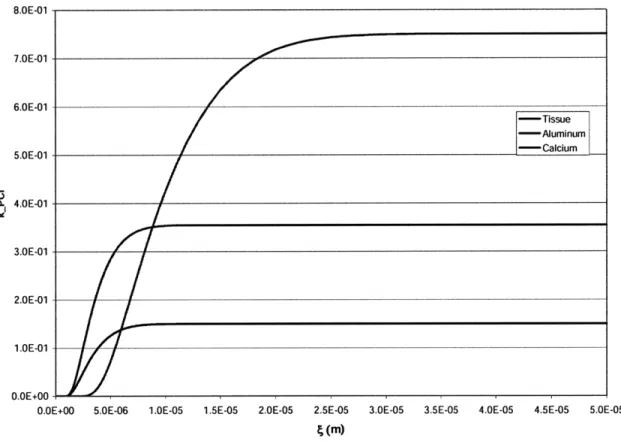
Conditions (17) and (19) ensure, across a sample, a degree of coherence that is in general considered good. It is interesting to note that both conditions describe a characteristic of the radiation source that is possible to modify. For transverse coherence length, the most common way to improve the coherence of the beam is to use a pinhole. By restricting the spatial extent of the source, i.e. reducing the beam divergence, we can theoretically achieve an arbitrarily long coherence length. This approach can be very costly in terms of the available flux, and with most x-ray sources it is in general infeasible to achieve a transverse coherence length in the sub-micrometer range. It is worth noticing though that most applications do not require a coherence length that extends to the entire sample. Imaging techniques using coherent beams are aimed at enhancing edges between materials. An edge is a step function and as such does not have an extent. Nevertheless, for the physical nature of the contact between two materials, we can consider the edge to have an extent, usually in the micrometer to sub-micrometer scale.

(32)

By properly restricting the x-ray source with a pinhole, and by positioning the sample at a suitable distance, suppose we build a system that, according to condition (17), has a AO narrow enough to ensure transverse coherence over features extending up to 5

tm. Condition (19) provides us then with a limit to the resolution of the imager when a polychromatic source is used. For instance, if the relatively narrow fractional bandwidth of 10-2 is used, a resolution greater (that is, worse) than 50 nm is available. This value falls significantly short of the resolution that is available in most microscopy imagers, such as an electron microscope. It is important to consider the wider scope of applications of x-ray imaging, due to the higher penetration of photons as compared to electrons, allowing the non-destructive probing of deeper samples. Furthermore, sample preparation is much simpler for x-ray imaging than for many electron-based imaging techniques.

The conditions discussed so far are independent of the sample and of the specific imaging technique where coherent radiation is required. Different techniques might have more specific requirements for the positioning of the sample and of the detector, and the overall resolution of an imager can vary depending on the specific design.

The transmission function q(x,y)

The discussion of the image formation process relied heavily on the transmission function q(x,y) as the term where all interactions between incoming radiation and the sample are accounted for. In other words, the ultimate goal of the image formation process is to provide us with a relationship between the image on the detector and the transmission function. Such a relationship can be as simple as a magnifying factor when ray-geometry can be considered valid, or as complicated as the interference patterns arising in the Fresnel regime of a coherent imager. The interest of such imaging systems lies in their ability to provide us insight into the properties of q(x,y).

A

definition of q(x,y)

A simple example of a transmission function is the description of a square aperture in an opaque screen in an optics experiment. Light impinges on the dark screen, and no

(33)

transmission happens except at the location of the square aperture. If the aperture has the width of 2a, we can write the transmission function as;

q(x,y) =I if -a<(y) (20)

0 otherwise

This formulation of the transmission function is common in optics problems involving apertures of various shapes restricting an incoming light source.

In the absence of the object the point (x,y) would emit a perfectly spherical

eikr

wavefront e, as per the Huygens-Fresnel principle. An object, however, would emit a

r

modified wavefront such as A- From these descriptions, we obtain a generic r

expression for the transmission function:

q(x, y) = A(x, y) e''x'Y). (21)

If we allow the term

4

to be complex, we can simplify the equation to:

q(x, y) = ei'(x'Y. (22)

The term contains all information about the interactions that the radiation will incur in the sample in its path from the source to the detector. We can expect that such interactions will have the effect of changing both the amplitude and the phase of the radiation. If we aggregate all phase changing effects in a single term 8, and all absorption effects in a single term 3, we can write:

0= (G + fl)dZ, (23)

where the integration is over the path of the photon in the sample. The quantities 6 and 3 are also used to define the index of refraction of a material:

(34)

n - " _ 1- +ip. (24) kout

We can see from equations (23) and (24) that there is a deep connection between the index of refraction of a material and its transmission function. This should not surprise us, since both quantities depend on the interaction of the radiation with matter. Before going further in the study of the terms 8 and

3,

we should look further into the interaction that can happen in an imaging system. Since we are primarily concerned with X-ray systems for medical diagnostics applications, we will focus on X-ray interactions with soft tissues.

Interaction of X-rays with matter

Our interest is in diagnostic radiography, that is, interaction of low energy photons (in general < 100keV) with low Z (atomic number) materials. In this range, three interaction modes of photons with matter are to be considered: photoelectric effect, Compton scattering and Rayleigh scattering.

a) Photoelectric effect

The photoelectric effect is described as the absorption of a photon by an atom. Upon absorption, the atom emits an electron and subsequently a characteristic photon (fluorescence). The absorption can happen only if the incoming photon has an energy equal to or higher than the binding energy of the electron to be ejected, most commonly the K-edge electron. The probability of the interaction between the incoming photon and the electron is maximal if the incoming photon has an energy that is close to that of the electron to be ejected, that is, close to the K-edge (or L-edge). This behavior is clearly visible in the discontinuous shape of the absorption coefficient close to the edge energies. Far from the edges, the probability of interaction is proportional to 1/E3, where E is the energy of the incoming photon. The probability of interaction is also proportional to Z3, where Z is the atomic number of the material.

(35)

In diagnostic radiography, the photoelectric effect is not the predominant interaction, except for x-rays of very low energy. For these applications, we can consider the fluorescence yield so low as to be neglected, and the photoelectric effect can be assumed to be purely absorption of photons in matter. Figure 7 shows how the importance of the photoelectric effect as compared to other effects decreases as the energy of the radiation increases in tissues. It also shows how in tissue and bone the K-edge is too small to be observable.

T- s isue Photoelectic effect

-*

-

-Tiue Compton scattering

---Bone Photoelectic effect

SB- Bone Compton scatedng

0

C 0.01

-0 20 40 60 80 100 120 140 160

Photon energy (keV)

Figure 7: Mass attenuation coefficient in tissue and bone. [7]

b) Compton scattering

Compton, or incoherent, scattering is usually described as the inelastic interaction of a photon with a free electron. Electrons in materials are in general bound to an atom, but if the energy of the incoming photon is much higher than the binding energy of the electron, the electron will "appear" free to the photon. Since the total scattering

(36)

process obeys conservation of energy and momentum, the scattered photon will be at a different wavelength than the incoming photon. The relationship between the wavelength of the scattered photon V', that of the incoming photon k, and the scattering angle 9 can be obtained through conservation equations, and is:

A'-1 = (1 - cos1) .

mec

The probability of interaction via Compton scattering is described by the Klein-Nishina formula. For non-relativistic photon energies, that is, much smaller than 511 keV, the Klein-Nishina formula converges with the Thompson formula, aside for a form factor that is due to the fact that the interacting electron is not free but is bound. We can then write the cross section for Compton scattering in the non-relativistic region as:

d(9)

Fc

c 2 _{(X(t9), Z)(1}

- cos2 t),

where x is the momentum transfer of the scattered photon, and F is a form factor that takes into account the fact that the interacting electron is bound to an atom that is in general also not free. The differential cross section as a function of ,9 in the non-relativistic case is relatively flat, that is, photons are approximately as likely to be scattered at a small forward angle as they are to be scattered at a large angle. The total cross section, obtained by integration of the Klein-Nishina formula over the entire solid angle, varies as 1/E and is independent from the atomic number of the interacting element, but is proportional to electron density of the material. Figure 7 shows how Compton scattering is the dominant interaction in tissue x-ray energies between 50keV and 100keV.

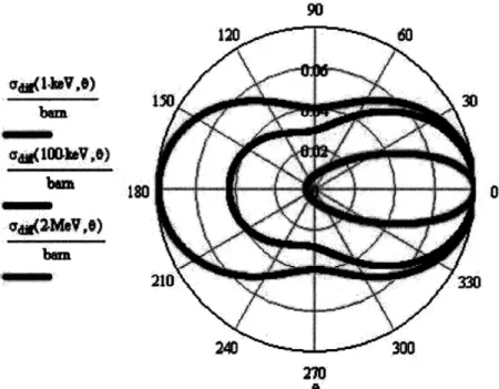
c) Rayleigh scattering

Coherent (Rayleigh) scattering is an elastic interaction between the photon and an atom where only the direction of the photon is affected, but not its energy. This apparent violation of conservation of energy is explained by the fact that the incoming photon is absorbed by the atom, which becomes unstable. The atom subsequently emits a photon of

(37)

the same energy as the photon that was absorbed. The scattered radiation is coherent, that is, it has the same wavelength as the incoming radiation, hence the name coherent scattering.

The differential scattering cross section for Rayleigh scattering can be written, similarly to non-relativistic Compton scattering, as:

d(9) oc Fcoh2((9), Z)(1 -cos2 9),

1 9

where x= - sin( ) is the momentum transfer. Since coherent scattering is by and large

A 2

an interaction involving the entire atom, the form factor is related to the electron charge distribution of the entire atom by means of a Fourier transform. For high momentum transfer x, that is, large angle scattering, only the most localized electrons contribute to the form factor. Since these electrons are not involved in interatomic bonding, a free atom approximation can be assumed. For low momentum transfer x, in general <0.25, the form factor will depend heavily on the bonding of the atoms with its neighbors. Thus, a measurement of Fcoh, or more simply of do/df, provides information about the structure of the material.

The differential scattering cross section has a dependence on 9 that favors small angles over large angles. At small angles the form factor is in general larger, and the differential scattering cross section is similar in shape to the Thompson scattering cross section. The Rayleigh differential cross section vanishes at large L9.

The total scattering cross section for Rayleigh scattering is for most radiological applications an order of magnitude lower than Compton scattering. Nevertheless, it would not be correct to discard the contribution of Rayleigh scattering to the interaction of x-ray radiation with matter. In fact, if we restrict our interest to small angle scattering of photons in the forward direction, Rayleigh scattering is much more prominent than Compton scattering. This is due to the fact that photons undergoing Compton interactions are scattered more or less uniformly over a large solid angle, while photons undergoing Rayleigh scattering are localized in a small cone around the forward direction. Figure 8