HAL Id: hal-00607296
https://hal.archives-ouvertes.fr/hal-00607296
Submitted on 8 Jul 2011
HAL is a multi-disciplinary open access
archive for the deposit and dissemination of
sci-entific research documents, whether they are
pub-lished or not. The documents may come from
teaching and research institutions in France or
abroad, or from public or private research centers.
L’archive ouverte pluridisciplinaire HAL, est
destinée au dépôt et à la diffusion de documents
scientifiques de niveau recherche, publiés ou non,
émanant des établissements d’enseignement et de
recherche français ou étrangers, des laboratoires
publics ou privés.
Kinetic Models and Qualitative Abstraction for
Relational Learning in Systems Biology
Gabriel Synnaeve, Katsumi Inoue, Andrei Doncescu, Hidetomo Nabeshima,
Yoshitaka Kameya, Masakazu Ishihata, Taisuke Sato
To cite this version:
Gabriel Synnaeve, Katsumi Inoue, Andrei Doncescu, Hidetomo Nabeshima, Yoshitaka Kameya, et al..
Kinetic Models and Qualitative Abstraction for Relational Learning in Systems Biology. BIOSTEC
Bioinformatics 2011, Jan 2011, Rome, Italy. �hal-00607296�
KINETIC MODELS AND QUALITATIVE ABSTRACTION FOR
RELATIONAL LEARNING IN SYSTEMS BIOLOGY
Gabriel Synnaeve
Katsumi Inoue
E-Motion Team at INRIA, Grenoble, France National Institute of Informatics, Tokyo, Japan [email protected] [email protected]
Andrei Doncescu
Hidetomo Nabeshima
LAAS-CNRS 31007, Toulouse, France University of Yamanashi, Japan [email protected] [email protected]
Yoshitaka Kameya, Masakazu Ishihata, Taisuke Sato
Tokyo Institute of Technology, Tokyo, Japan
{kameya,ishihata,sato}@mi.cs.titech.ac.jp
Keywords: systems biology, discretization, metabolic pathways, inductive logic programming, abduction
Abstract: This paper presents a method for enabling the relational learning or inductive logic programming (ILP)
frame-work to deal with quantitative information from experimental data in systems biology. The study of systems biology through ILP aims at improving the understanding of the physiological state of the cell and the interpre-tation of the interactions between metabolites and signaling networks. A logical model of the glycolysis and pentose phosphate pathways of E. Coli is proposed to support our method description. We explain our original approach to building a symbolic model applied to kinetics based on Michaelis-Menten equation, starting with the discretization of the changes in concentration of some of the metabolites over time into relevant levels. We can then use them in our ILP-based model. Logical formulae on concentrations of some metabolites, which could not be measured during the dynamic state, are produced through logical abduction. Finally, as this re-sults in a large number of hypotheses, they are ranked with an expectation maximization algorithm working on binary decision diagrams.
INTRODUCTION
Nowadays, systems biology represents the key field to explain the functionality of life science. To ana-lyze a biological system it is necessary to find out new mathematical models allowing to explain the evolu-tion of the system in a dynamic context or to deal in a simple manner with the complex situations where the human experience overtakes mathematical reasoning (Kitano, 2002). Many physical and biological phe-nomena may be represented on an analytical form us-ing dynamical system. Our case study is based on wet biology experiment consisting in applying a pulse of glucose in a small bio-reactor containing E.Coli that led to building an ordinary differential equations (ODEs) based simulator. We used high performance liquid chromatography to measure some metabolites concentrations and some others had to be estimated, using a simulated annealing algorithm, since no ex-perimental results were available. So, knowing com-pletely the evolutions of metabolites concentrations of this system, we applied our approach to show its cor-rectness. For that, we took only steady-state values of
metabolites concentrations and ran our model. Several attemps have been done for logic-based approaches to analyze biochemical pathways in Sys-tems Biology. They use action languages (Baral et al., 2004), abduction (Juvan et al., 2005; King et al., 2004; King et al., 2005; Tamaddoni-Nezhad et al., 2006), SAT (Tiwari et al., 2007), inductive logic gramming (Doncescu et al., 2007) or answer set pro-gramming (Dworschak et al., 2008). All these pre-vious approaches are based on qualitative modeling, and none of them can handle continuous domains ap-propriately. Temporal logic combined with the rep-resentation of kinetic models in stochastic logic pro-gramming (SLP) (Fages et al., 2008) have a simi-lar goal using different means: the authors modeled the kinetics of biochemical systems by continuous time Markov chains as input to SLP where we took an approach to discretize (through continuous HMM) concentrations of metabolites first and then use them combined with a logical translation of ODEs-based kinetics as input to ILP. The goal of this research is to incorporate continuous values and kinetics within the logic-based approach to metabolic pathways. In
particular, we enhance an abductive framework pro-posed in (Inoue et al., 2009), which consists of ab-ductive hypothesis generation and statistical hypoth-esis evaluation, by enabling us to handle real-valued data obtained from measurement in observations.
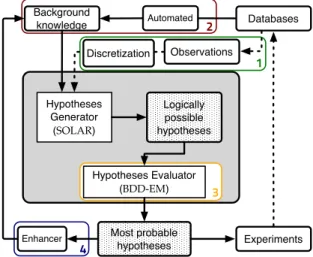
For that, we now propose a loop for learning
about a metabolic pathway from experimentsin which we have to (each step corresponds to a section, as in Fig. 1):
1. clusterize continuous concentrations of metabo-lites over time into discrete levels and discrete timesteps.
2. use them in an ILP-based model of the pathway, in conjunction with a set of knowledge-generating rules, here in the example describing Michaelis-Menten kinetics.
3. sort the resulting abduced facts or inducted rules with our defined metrics.
4. use this ranking for enhancing our knowledge base and goto the beginning of this process.
4 Experiments Logically possible hypotheses Databases Hypotheses Generator (SOLAR) Hypotheses Evaluator (BDD-EM) Background knowledge Observations Most probable hypotheses 3 Discretization Automated Enhancer 1 2
Figure 1: Overview of the complete process
In this paper, we show how this “closed loop” architecture can be applied to an inverse problem: given the measured concentrations of some metabo-lites in a steady state, we compute the concentra-tions of metabolites before the dynamic transition to this steady state based on the kinetic modeling. We worked with the beginning of an automated frame-work (see Fig. 2 for a practical data-centric circuit) to deal with different real world pathways and exper-iments. It is mainly composed of four tools:
• The combination of an implementation of contin-uous HMMs (Gauvain and Lee, 1994; Ji et al., 2006) withPY-TSDISCto discretize experimental values.
• KEGG2SYMB, using the KEGG API, that trans-form pathways from KEGG (Kanehisa and Goto, 2000; Kanehisa et al., 2008) into symbolic mod-els.
• SOLAR, a consequence finding system working on Skipping Ordered Linear tableaux (Nabeshima et al., 2003), which is complete for finding mini-mal explanations, to conduct abduction or induc-tion.
• BDD-EM, an implementation of the expectation-maximization algorithm on binary decision dia-grams (Ishihata et al., 2008; Inoue et al., 2009) to rank hypotheses.
We chose to illustrate this method on the conjunc-tion of glycolysis and pentose phosphate pathways for
E.Coli, simplified the model by keeping 16 relevant reactions and discretized experimental values (16 val-ues) as in section 1. We added the three Michaelis-Menten based rules and the three constraints of unic-ity for the levels as in section 2. We had 15 un-known levels of concentrations of metabolites before the transition to the steady state (yielding 15×3 levels = 45 abducibles).SOLAR, used for abduction, outputs 98 hypotheses that cover all these metabolites. With such a number, picking the right hypotheses should be done in an automated way as we did in section 3.
KEGG
Experimental Data
kegg2symb Symbolicpathway
py-tsdisc HUP SOLAR Discretized data Kinetic rules BDD-EM Hypotheses Ranked hypotheses : append enhancer New KB rules generator
Figure 2: Data-centric schema of the process
1
DISCRETIZATION OF TIME
SERIES FROM EXPERIMENTS
In our modeling, we first introduce discrete concen-tration levels to filter what are the relevant changes of concentration of the metabolites, in regard to hy-potheses generation from ILP. We need to be able to infer hypotheses that have a certain level of generality and, for that, we should use intervals instead of single real values. This could have been done with an inter-val constraints approach (Benhamou, 1994), but we currently choose a discretization approach. Although this gives us less freedom in the logic part as levels
are fixed (as if we have fixed intervals), levels can be handled just as symbols in a logical model of path-ways.
Discretizing time series is a research field in which many works (Geurts, 2001; Keogh et al., 2005) have been conducted recently. Our practical problem is that we want to have a statistically relevant (unsupervised) discretization for N metabolites concentrations over time. We also discretize the values of Km
(Michaelis-Menten constants, see (1)), for each reaction, with the same levels. For that purpose, we use a probabilis-tic model, used in speech recognition and time series analysis: continuous hidden Markov model (HMMs) (Rabiner, 1989). We can therefore compute an ap-propriate number of levels (that was three for E.Coli) in regard to a Bayesian score such as Bayesian In-formation Criterion (BIC) (Schwarz, 1978) or as the Cheeseman-Stutz score (Cheeseman and Stutz, 1995) or as the variational free energy. This process can be achieved through the following methods all de-scribed in (Beal, 2003), respectively: maximum like-lihood estimation or maximum a posteriori estimation or through a variational Bayesian method.
We use continuous (Gaussian) HMMs with pa-rameter tying1. This is a solution to the problem of sharing the same symbolic levels in all the logic mod-els in order to be able to assign the level of a com-pound to another and be dealing with the same real values behind the scene. We first prepare N contin-uous HMMs (one for each metabolite), where each state variable takes a concentration level, and each output variable takes a measurement of concentration and follows a univariate Gaussian distribution. All the HMMs share a state space as well as the parameters in the output variables (i.e. means and variances), so that they produce discrete levels that are correspond-ing. These relevant discretized levels of concentration are computed through the expectation-maximisation (EM) algorithm with maximum a posteriori (MAP) estimation (Gauvain and Lee, 1994) or through the variational Bayes EM (VB-EM) (Beal, 2003; Ji et al., 2006). We prefer this last method as it is shown (Beal, 2003) that variational free energy provides a more ac-curate approximation of the marginal log-likelihood than BIC or the Cheeseman-Stutz score.
Then, we use a simple round-mean aggregation of them for time-sampling. We set a maximal number
1Parameter tying is a notion often used in HMMs for
speech recognition (Rabiner, 1989) and recently in statisti-cal relational learning (De Raedt, 2008). In our case, the mean and the variance for Xt(n), the output variable at time
t in the HMM for the n-th metabolite (n= 1, . . . , N), are tied with the mean and the variance for X(n
′)
t′ , respectively (n6= n′and t6= t′).
Figure 3: 3-state continuous HMM discretizing one experi-mental time series, where Xtis the measurement of
concen-tration at time t and Stis the hidden state that indicates the
corresponding discretized level.
of time steps and look for the better fitting width and alignment for equal-width time intervals. We are cur-rently developping a different process in the direction of discretization of our time series from molecular bi-ology experiments that will discretize time and levels simultaneously but current results are already useable (see Table 1 and Fig. 5 ) and that is what we based the work presented here on.
2
MODELING OF THE
PATHWAYS OF E.COLI
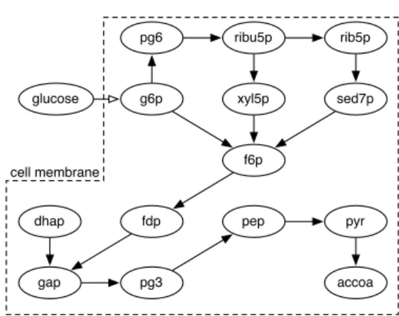
To obtain an understanding of the central metabolism, a logical model has been developed according to a kinetic model including the glycolysis and the pen-tose phosphate pathway for Escherichia coli (Chas-sagnole et al., 2006). The Fig.4 shows the simplified pathway that we modelized logically with relations
reaction(Substrate, Enzyme, Product, Km).
pg6 ribu5p rib5p
glucose g6p xyl5p sed7p
f6p
dhap fdp pep pyr
gap pg3 accoa
cell membrane
Figure 4: Simplified glycolysis and pentose phosphate path-ways for E.Coli
The metabolic networks dynamics are in their en-zymatic part ruled by the combination of classical kinetics: essentially Michaelis-Menten, Hill and al-losteric ones. If we limit our modeling to these kinet-ics, we can highly simplify their mathematical
han-dling, and that is what we did. We chose to use only Michaelis-Menten kinetics, because we had a path-way simple enough and that it is the more general rep-resentation for a non-linear allosteric regulation sys-tem. It assumes that the two enzyme binding equi-libria are fast when compared to the interconversion of enzyme + substrate (ES) and enzyme + product (EP) compounds. That assumption appears reason-able considering that the dynamics of the experiment were happening in less that a minute: this implies that the effects of genetic regulation of the enzymes in-cluded are negligible and so the maximum reaction rates represent the amount and catalytic activity of en-zymes.
E+ S ⇋k1
k−1ES→
k2E+ P
Michaelis− Menten eq. : d[P]
dt = Vm
[S] [S] + Km
(1) If both the substrate (S) and the product (P) are present, neither can saturate the enzyme. For any given concentration of S the fraction of S bound to the enzyme is reduced by increasing the concentra-tion of P and vice versa. For any concentraconcentra-tion of P, the fraction of P bound to the enzyme is reduced by increasing concentration of S. When we have S ⇆ P, we just have to consider reactions for both directions. We consider a time discretization of the chemical rate equation for a reation between a substrate and a prod-uct with respective stoechiometric coefficient s and p:
s.S → p.P : rate =1 p× d[P] dt −→disc.time 1 p× ∆[P] ∆T (2) (1) and (2) =⇒ p × rate = Vm [S]T [S]T+ Km ≈ [P]T+timestep− [P]T (T + timestep) − T
We chose to work with a constant timestep : =⇒ [P]T+1= Vm
[S]T
[S]T+ Km
+ [P]T (3)
We can note that the Michaelis-Menten constants (Km) are homogenous to a concentration. We can then state conc(Km, Level, Time) in our modeling to set them, where conc stands for concentration. The experimental response observations of intra-cellular metabolites to a pulse of glucose were measured in continuous culture employing automatic stopped flow and manual fast sampling techniques in the time-span of seconds and milliseconds af-ter the stimulus with glucose. The extracellular glucose, the intracellular metabolites: glucose-6-phosphate (g6p), fructose-6-phosphate (f6p),
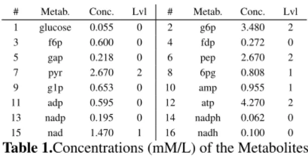
fructose1-6bisphosphate (fdp), glyceralde-hyde3phosphate (gap), phospho-enolpyruvate (pep), pyruvate (pyr), 6phosphate-gluconate (6pg), glucose-1-phosphate (g1p) as well as the cometabolites: atp, adp, amp, nad, nadh, nadp, nadph were measured using enzymatic methods or high performance liquid chromatography. All the steady-state concentrations
measurements of the E.Coli experiment and their corresponding discrete levels are summarized in Table 1.
# Metab. Conc. Lvl # Metab. Conc. Lvl 1 glucose 0.055 0 2 g6p 3.480 2 3 f6p 0.600 0 4 fdp 0.272 0 5 gap 0.218 0 6 pep 2.670 2 7 pyr 2.670 2 8 6pg 0.808 1 9 g1p 0.653 0 10 amp 0.955 1 11 adp 0.595 0 12 atp 4.270 2 13 nadp 0.195 0 14 nadph 0.062 0 15 nad 1.470 1 16 nadh 0.100 0
Table 1.Concentrations (mM/L) of the Metabolites and their discretized levels for steady states Inductive Logic Programming, used for induction or abduction (Mooney, 1997), allows to deal with dis-crete levels (symbols) and qualitative rules (Doncescu et al., 2007). Given the background knowledge B and an observation E (example), the task of ILP is to find an hypothesis H such that:
• B ∧ H |= E and • B ∧ H is consistent
Inverse entailment (Inoue, 1992; Muggleton, 1995; Inoue, 2004) enables us to compute H through de-duction by using:
• B ∧ ¬E |= ¬H and • B 2 ¬H
We are here interested in abducing what happens during the dynamical transition based on observations from Table 1. Inverse entailment for abduction is studied in (Inoue, 1992) in which abductive computa-tion can be realized by the consequence finding pro-cedure SOL. In this case, both E and H are sets of lit-erals, so both¬E and ¬H are clauses. This approach can be further extended for inducing general hypothe-ses in (Inoue, 2004), which is generalized from (Mug-gleton, 1995), to allow B, E and H for full clausal theories.
SOLARcan be used as an abductive procedure to infer a hypothesis H in the form of a set of liter-als. Our logical model is based on the simplified Michaelis-Menten equation (3) which has here been represented by three background clauses using the conc(Compound, Level, Time) predicate. If we make the approximations for extreme values in:
[P]T+1= Vm
[S]T
[S]T+ Km
With only 3 levels, as we have in our discretization of
E.Coliexperiments, we will get the following simple rules: • [S] ≪ Km⇒ ∆[P] ∆T = Vm KM⇒ [P]T+1= [P]Treaction(S, P, Km) ∧ conc(S, 0, T) ∧ conc(Km, 2, T) ∧ conc(P, L, T) → conc(P, L, T+1)
The concentration of the product will not change between T and T+1 if the reaction is very slow.
• [S] ≃ Km ⇒ ∆[P] ∆T = Vm 2 ⇒ [P]T+1 = Vm/2 + [P]T reaction(S, P, Km) ∧ conc(S, L, T) ∧ conc(Km, L, T) ∧ conc(P, L2, T) → conc(P, L2, T+1)
The concentration change of the product between T and T+1 is not big enough to switch from one level to another. This is an approximation and a handy consequence of our discretization (using a log-scale on real values).
• [S] ≫ Km ⇒ ∆[P] ∆T = Vm ⇒ [P]T+1 = Vm+ [P]T reaction(S, P, Km) ∧ conc(S, 2, T) ∧ conc(Km, 0, T) ∧ conc(P, L, T) → conc(P, 2, T+1)
If the reaction is very quick, it will result in trans-forming all the substrate into product in one time step.
If we had more than three levels, we would either need more rules (they can be automatically generated) or a general procedure for handling our kinetic model. This last one is a current implementation issue related toSOLAR. Another way to deal with more levels
be-ing currently explored consist in the automated gen-eration of kinetics rules w.r.t. the discretization. Fur-thermore, we made some simplifications in the path-ways to be able to use only Michaelis-Menten kinet-ics, another research topic is to extend our modeling to reactions ruled by other types of kinetics.
We also added constraints about the unicity of lev-els at a given time to reduce the number of hypotheses while keeping consistency:
• ¬conc(S, 0, T) ∨ ¬conc(S, 1, T) • ¬conc(S, 0, T) ∨ ¬conc(S, 2, T) • ¬conc(S, 1, T) ∨ ¬conc(S, 2, T)
Now we set the observations for the 6 metabo-lites (#2 - #7) from Table 1, which have been possibly affected by the stimulus with glucose, and the abducibles as those literals of the form
conc( , ,0). Using SOLAR, we get 98
hypothe-ses as: H76 = conc(g6p,2,0) ∧ conc(adp,2,0) ∧ conc(fdp,0,0) ∧ conc(dhap,0,0) ∧
conc(gap,0,0) ∧ conc(glucose,2,0) ∧
conc(pg3,2,0) ∧ conc(pep,2,0) ∧ conc(atp,0,0)
∧ conc(pyr,2,0)
3
RANKING HYPOTHESES
(Ishihata et al., 2008) (Ishihata et al., 2008) pro-posed the BDD-EM algorithm that is an implementa-tion of the expectaimplementa-tion maximizaimplementa-tion algorithm work-ing on binary decision diagram, allowwork-ing it to deal with boolean functions. (Inoue et al., 2009) (Inoue et al., 2009) have applied the BDD-EM algorithm to rank hypotheses obtained through abduction. To rank our H1, . . . , Hnhypotheses by probability, we consider
the finite set of ground atoms
A
that contains all the values that can take our conc(Compound, Level, Time) and reaction(Substrate, Product, Km). Each of the elements ofA
is a boolean variable. One of its subsets is the subset of abducibles Γ com-posed of all the possible values of conc(Compounds, Level, 0). With θi= P(Ai) f or Ai∈A
, we haveto maximize the probability of the disjunction of hy-potheses helped with the background knowledge B:
F= (H1∨ · · · ∨ Hn) ∧ ground(B) to set the good θ
pa-rameters (by the BDD-EM algorithm). F can still be too big to be retained as a BDD, so an optimisation F′ of its size is obtained through the use of the minimal proofs for B and each Hi. Then, the BDD-EM
algo-rithm computes the probabilities of ground atoms in
A
that maximizes the probability of F′. Finally, the probabilities of each hypotheses used for the ranking are computed as the products of the probabilities of literals appearing in each Hi.To sort our 98 abduced hypotheses, we ran the EM algorithm on the BDDs corresponding to our hypothe-ses 10,000 times with random initializations. Note that if the comparison of these probabilities with each other is relevant, they should not be taken as abso-lute probabilities. The 10 most probable abduced hy-potheses are the following:
Hyp. # Probability Abduced conc. levels at T=0
H76 ≈ 1.000 g6p: 2, adp: 2, f6p: 0, fdp: 0,
dhap: 0, gap: 0, glucose: 2, pg3: 2, pep: 2, atp: 0, pyr: 2
H41 0.822 the same as H76 except pg3: 0
H56 0.625 the same as H76 except g6p: 0
H70 0.553 the same as H76 except atp: 2
H13 0.515 the same as H56 except adp: 0
H90 0.455 the same as H70 except pg3: 0
H82 0.442 the same as H76 except dhap: 2
H43 0.369 the same as H76 except pyr: 1
H9 0.364 the same as H41 except dhap: 2
H68 0.346 g6p: 0, adp: 0, f6p: 0, fdp: 0,
dhap: 0, gap: 0, glucose: 2, pg3: 2, pep: 2, atp: 2
Table 2. 10 most probable hypotheses These hypotheses are corresponding to our biolog-ical knowledge that pyruvate is a bottleneck (Peters-Wendisch et al., 2001) and that the glucose that is
to-Figure 5: Top: Discretization of the concentration of glu-cose in the Glycolysis Pathway of E.Coli after an initial pulse. Bottom: Simulated evolution of the concentration of fructose-6-phosphate during the whole experiment.
tally consumed (e.g. top plot of Fig. 5 from simula-tion) was in high concentration at the beginning of the experiment (pulse). It goes along with the very gen-eral reaction of glycolysis: glucose+ 2ADP + 2P + 2NAD+ → 2 pyruvate + 2ATP + 2(NADH, H+) +
2H2O. Also, for some metabolites, such as
fructose-6-phosphate, the levels found through abduction are corresponding to the output of the simulation (e.g bot-tom plot of Fig.5) with the same low level (0) before and after the dynamic transition.
4
ENHANCING THE
KNOWLEDGE BASE
Increasing our knowledge about a system is consid-ered as an iterative process: at first, we consider the background knowledge combined with the observa-tions as our knowledge base. Then we produce hy-potheses and we need to use an algorithm to enhance (update) our knowledge base with some of the discov-ered hypotheses, here: abducibles. Ideally, we would re-run the hypothesis finding process until we can-not find anything new. This is particularly important when working with complex chained reactions and multiple time steps as it can enable deeper learning.
This idea of revising the knowledge base is already found in (Ray et al., 2009) with a nonmonotonic ap-proach, but their revision method stays in a qualitative modeling and do not take quantitative aspects into ac-count.
Here, it is needed to pick hypotheses that are con-sistent with the background knowledge and with each others. For example, if we apply a greedy algorithm (as Algorithm 1) that picks hypothesis in decreasing probability order such that the hypothesis add some knowledge and that our enhanced knowledge stays consistent, it prevents from abducing other discover-ables than the ones contained in H76. For instance we cannot find concentrations at T=0 for ribu5p, rib5p, sed7p, xyl5p, because if they were abduced, the re-sulting hypotheses would become inconsistent with H76. Note also that the abducibles added into the knowledge base may reduce the computational cost of later iterations of abduction/induction, but it is com-parable to discard some branches of exploration. Algorithm 1 An algorithm to enhance the knowledge base: most probables firsts
knowledge← knowledge base
sorted hypotheses← sort(hypotheses)
while length(discoverable)> 0 &&
length(sorted hypotheses)> 0 do
tmp← sorted hypotheses.pop()
if contains(tmp, discoverable) && consistent(tmp, knowledge) then
knowledge.enhance(tmp) discoverable.remove(tmp) end if
end while
With the explicit functions length, pop (destructive), and: • sort sorts the hypotheses by decreasing probability. • contains is a function that returns statements of first
ar-gument contained in the second.
• consistent performs consistency checking of two theo-ries and return True if they are consistent.
• enhance adds statements that are not yet present in the considered (“self”, “this”) knowledge.
• remove deletes statements from argument present in the considered (“self”, “this”) object (could make use of
contains).
We could have chosen to pick a combination of hypotheses that discovers more abducibles by penal-izing the solutions including too few different ab-ducibles with a scoring function inspired by the BIC (Schwarz, 1978): score= −2 ln(error) + λ · f (k, n) with k being the number of chosen hypotheses, n the number of abducibles, f a function that indicates the structural complexity of the combination of hypothe-ses (decreasing with the increase of n and increasing with the increase of k) and error the product of the
probabilities of chosen hypotheses. We assume here that we can use their relative significations in error by unbiasing the score with a λ parameter. So that the goal of such an algorithm would be to discover all abducibles while minimizing this score.
CONCLUSION
As we found that our results (for time T=0) agreed with existing background knowledge in biology and our ODEs-based simulator, this paper showed a method to deal with the kinetics of metabolic path-ways with a symbolic model (i.e. Fig 1). We ex-plained how to discretize biology experiments into relevant levels to be used with ILP and logic programs in the large. Moreover, based on these discretization of concentration into levels, we explained our pro-cess to transform Michaelis-Menten analytical kinet-ics equation into logic rules, the authors are not aware of any previous work in this direction. Therefore the originality of the work is given by the capacity of a logical model to find the dynamic response of micro-organism when a pulse of glucose has been made. We think that this approach improves the accuracy of the metabolic flux analysis. Allowing for other kinds of kinetic modeling (two substrate and/or two products reactions) would enable us to work with more com-plete models.
As in (King et al., 2005), this approach tries to study the behaviour of many ordinary differential equations while considering a symbolic model with its advantages whereof the statistical evaluation of potheses. The process of statistically evaluating hy-potheses, thanks to BDD-EM (Inoue et al., 2009), is seen as a good method to find relevant knowledge among the large quantity of processed data. The prac-tical validity of this full process (including discretiza-tion) has been shown by the results of this paper while working in a well-known theoretical framework (In-oue, 2004; Mooney, 1997). We strongly believe that the use of time series discretization and a kinetic mod-eling to enable ILP to deal with ODE will yield great results. We also prefer to consider knowledge dis-covery as an iterative loop where one must review his knowledge base in the light of new findings (i.e. add “New KB” next turn in Fig. 2).
Still, our modeling can be improved, and time and concentration discretization could be finer. Experi-ments dealing with more than 3 levels and many time steps will be lead on the Glycolysis and Pentose Phos-phate pathways of another bacteria, Saccharomyces
Cerevisiae (yeast), with both real world data from experiments and simulated data. More experiments
with enhancing and updating the knowledge base on this dataset is necessary to get more accurate results. A more global approach of discretizing experimental data and using it in conjunction with automatically generated symbolic pathways extracted from KEGG (Kanehisa and Goto, 2000; Kanehisa et al., 2008) can be applied regardless of the model chosen for infering new knowledge. This approach can be generically ap-plied to turn quantitative results from systems biology into qualitative (symbolic) ones.
REFERENCES
Baral, C., Chancellor, K., Tran, N., Tran, N., Joy, A., and Berens, M. (2004). A knowledge based approach for representing and reasoning about signaling networks. In Proc. of the 12th Int. Conf. on Intelligent Systems
for Molecular Biology, pages 15–22.
Beal, M. (2003). Variational Algorithms for Approximate
Bayesian Inference. PhD thesis, Gatsby Comp. Neu-rosc. Unit, University College London.
Benhamou, F. (1994). Interval constraint logic program-ming. Lecture Notes in Computer Science, 910. Chassagnole, C., Rodrigues, J., Doncescu, A., and Yang,
L. T. (2006). Differential evolutionary algorithms for
in vivo dynamic analysis of glycolysis and pentose phosphate pathway in Escherichia Coli. A. Zomaya. Cheeseman, P. and Stutz, J. (1995). Bayesian
classifica-tion (autoclass): Theory and results. In Advances in
Knowledge Discovery and Data Mining, pages 153– 180. The MIT Press.
De Raedt, L. (2008). Logical and Relational Learning.
Springer.
Doncescu, A., Yamamoto, Y., and Inoue, K. (2007). Biolog-ical systems analysis using Inductive Logic Program-ming. In IEEE International Symp. on Bioinf. and Life
Science Computing.
Dworschak, S., Grell, S., Nikiforova, V., Schaub, T., and Selbig, J. (2008). Modeling biological networks by action languages via answer set programming.
Con-straints, 13(1/2):21–65.
Fages, F., Soliman, S., and France, I. R. (2008). Model revision from temporal logic properties in systems bi-ology. In In: Probabilistic Inductive Logic
Program-ming. LNAI, volume 4911, pages 287–304.
Gauvain, J.-L. and Lee, C.-H. (1994). Maximum a poste-riori estimation for multivariate gaussian mixture ob-servations of markov chains. IEEE Transactions on
Speech and Audio Processing, 2(2):291–298. Geurts, P. (2001). Pattern extraction for time-series
clas-sification. Lecture Notes in Artificial Intelligence, 2168:115–127.
Inoue, K. (1992). Linear resolution for consequence find-ing. Artificial Intelligence, 56:301–353.
Inoue, K. (2004). Induction as consequence finding.
Inoue, K., Sato, T., Ishihata, M., Kameya, Y., and Nabeshima, H. (2009). Evaluating abductive hypothe-ses using and EM algorithm on BDDs. In Proc. of
IJCAI-09, pages 820–815. AAAI Press.
Ishihata, M., Kameya, Y., Sato, T., and Minato, S. (2008). Propositionalizing the EM algorith by BDDs. Tech-nical report, TR08-0004, Dept. Comp. Sc., Tokyo In-stute of Technology.
Ji, S., Krishnapuram, B., and Carin, L. (2006).
Varia-tional bayes for continuous hidden markov models and its application to active learning. IEEE
Transac-tions on Pattern Analysis and Machine Intelligence, 28(4):522–532.
Juvan, P., Demsar, J., Shaulsky, G., and Zupan, B. (2005). Genepath: from mutations to genetic networks and back. Nucleic Acids Res., 33.
Kanehisa, M., Araki, M., Goto, S., Hattori, M., Hirakawa, M., Itoh, M., Katayama, T., Kawashima, S., Okuda, S., Tokimatsu, T., and Yamanishi, Y. (2008). KEGG for linking genomes to life and the environment.
Nu-cleic Acids Res., 36:480–484.
Kanehisa, M. and Goto, S. (2000). Kyoto encyclopedia of genes and genomes. Nucleic Acids Res., 28(1):27–30. Keogh, E., Lin, J., and Fu, A. (2005). HOT SAX: efficiently finding the most unusual time series subsequence. In
5th IEEE International Conference on Data Mining.
King, R., Garrett, S., and Coghill, G. (2005). On the
use of qualitative reasoning to simulate and iden-tify metabolic pathways. Bioinformatics, 21(9):2017– 2026.
King, R., Whelan, K., Jones, F., Reiser, P., Bryant, C., Mug-gleton, S., Kell, D., and Olivier, S. (2004). Functional genomic hypothesis generation and experimentation by a robot scientist. Nature, 427:247–252.
Kitano, H. (2002). Systems biology toward
system-level understanding of biological systems. Science, 295(5560):1662–1664.
Mooney, R. (1997). Integrating abduction and induction in machine learning. In Working Notes of the IJCAI97
Workshop on Abduction and Induction in AI, pages 37–42.
Muggleton, S. (1995). Inverse entailment and progol. New
Generation Computing, 13(3/4):245–286.
Nabeshima, H., Iwanuma, K., and Inoue, K. (2003). SO-LAR: A consequence finding system for advanced reasoning. In Proc. of the 11th International
Con-ference TABLEAUX 2003, LNAI, volume 2786, pages 257–263.
Peters-Wendisch, P., Schiel, B., Wendisch, V., and et al.,
E. K. (2001). Pyruvate carboxylase is a major
bottleneck for glutamate and lysine production by corynebacterium glutamicum. Molecular Microbiol.
Biotechnol., 3(2).
Rabiner, L. (1989). A tutorial on hidden markov models and selected applications in speech recognition. Proc.
of the IEEE, 77(2):257–286.
Ray, O., Whelan, K., and King, R. (2009). A nonmonotonic logical approach for modelling and revising metabolic
networks. Complex, Intelligent and Software Intensive
Systems, IEEE.
Schwarz, G. (1978). Estimating the dimension of a model.
Annals of Statistics, 6(2):461–464.
Tamaddoni-Nezhad, A., Chaleil, R., Kakas, A., and Mug-gleton, S. (2006). Application of abductive ILP to learning metabolic network inhibition from temporal data. Machine Learning, 64:209–230.
Tiwari, A., Talcott, C., Knapp, M., Lincoln, P., and
Lader-oute, K. (2007). Analyzing pathways using
SAT-based approaches. In Proc of the 2nd Int. Conf. on