READ THESE TERMS AND CONDITIONS CAREFULLY BEFORE USING THIS WEBSITE.
https://nrc-publications.canada.ca/eng/copyright
Vous avez des questions? Nous pouvons vous aider. Pour communiquer directement avec un auteur, consultez la première page de la revue dans laquelle son article a été publié afin de trouver ses coordonnées. Si vous n’arrivez pas à les repérer, communiquez avec nous à [email protected].
Questions? Contact the NRC Publications Archive team at
[email protected]. If you wish to email the authors directly, please see the first page of the publication for their contact information.
Archives des publications du CNRC
Access and use of this website and the material on it are subject to the Terms and Conditions set forth at
A Multiple DSP-based 3D Laser Range Sensor and its Application to
Real-time Motion Detection
Green, David; Blais, François
https://publications-cnrc.canada.ca/fra/droits
L’accès à ce site Web et l’utilisation de son contenu sont assujettis aux conditions présentées dans le site
LISEZ CES CONDITIONS ATTENTIVEMENT AVANT D’UTILISER CE SITE WEB.
NRC Publications Record / Notice d'Archives des publications de CNRC:
https://nrc-publications.canada.ca/eng/view/object/?id=fb735529-af7b-453e-b53f-453ea8065ea0
https://publications-cnrc.canada.ca/fra/voir/objet/?id=fb735529-af7b-453e-b53f-453ea8065ea0
Institute for
Information Technology
Institut de technologie
de l’information
A Multiple DSP-based 3D Laser Range Sensor and its
Application to Real-time Motion Detection.
*
Green, D., and Blais, F.
May 2002
* published in: NRC/ERB-1095. May 2002, 201 pages.
Copyright 2002 by
National Research Council of Canada
Permission is granted to quote short excerpts and to reproduce figures and tables from this report, provided that the source of such material is fully acknowledged.
Institute for
Information Technology
Institut de technologie
de l’information
A M ult iple DSP-ba se d 3 D
La se r Ra nge Se nsor a nd it s
Applic a t ion t o Re a l-t im e
M ot ion De t e c t ion.
Green, D., and Blais, F.
May 2002
Copyright 2002 by
National Research Council of Canada
Permission is granted to quote short excerpts and to reproduce figures and tables from this report, provided that the source of such material is fully acknowledged.
Table of Contents
TABLE OF CONTENTS ...1
LIST OF FIGURES ...3
ABSTRACT...4
1.
INTRODUCTION ...4
2.
PRINCIPLE OF OPERATION...5
2.1.
Scanner Operation for Motion Detection... 5
2.2.
Motion Detection ... 7
2.3.
Data Presentation ... 8
3.
THE USER INTERFACE FOR THE DEMONSTRATION SYSTEM...8
3.1
The Waveform Controller Form... 8
3.2
Waveform List ... 10
3.3
Waveform Adjust ... 11
3.4
Motion Parameters ... 11
3.5
Display Parameters ... 11
4.
HARDWARE CONFIGURATION...14
4.1
The Desktop PC ... 17
4.2
The modular DSP (MDSP) system... 17
4.3
The Prototype Laser Scanner... 19
4.4
The Scanner PC Interface Electronics ... 19
5.4
The Peak Detector and Galvo Control DSPs ... 28
5.5
3DMD System Task Configuration... 29
5.6
Summary of System-wide Message Passing ... 32
5.7
Task Creation Sequence at Startup ... 34
5.8
Communications Aspects of the User Interface Software ... 35
6.
THE MDSP DEVELOPMENT ENVIRONMENT ...36
6.1.
Software Development with MQX ... 36
6.2.
Debugging a Multiprocessor System with Code Composer Studio ... 37
6.3.
System Startup... 38
6.4.
Software Development Tools ... 38
6.5.
Managing Complexity of MDSP Software Development... 39
7.
HOW TO RUN THE DEMONSTRATION ...40
8.
RESULTS ...44
9.
CONCLUSIONS ...45
10. REFERENCES ...46
11. APPENDIX...47
Appendix A. Code Listings of Real-time DSP Software... 48
Appendix B. Code listings for the Peak M62 and Galvo M62 DSPs ... 118
Appendix C. The User Interface Software. ... 162
Appendix D. Installing Precise/MQX on a Q67 or M62 DSP Platform... 184
Installation and testing of MQX2.40
... 184
A.
Install PSP and BSP... 185
B.
Update the PSP ... 185
C.
Build the PSP... 187
D.
Verify DOS environment variables ... 187
E.
Modify the BSP ... 187
F.
Build BSP ... 191
G.
Test the Installation ... 192
H.
Setup Code Composer Studio Environment... 192
I.
Adding I/O support for Innovative’s PCI-based terminal emulator. ... 193
J.
CodeWright Upgrade (Vers. 6.0b to 6.0#) ... 195
L.
Synchronizing Code Composer Studio with CodeWright (Optional) ... 195
M.
Using the Code Composer Studio Development Environment (Optional) ... 196
N.
Installing Precise Solution ... 196
O.
Installing MQX Task Aware Debugging Plug-in for Code Composer Studio... 196
P.
Required Patches after Reinstalling the Q67 Development Package ... 196
Q.
Special Note Regarding Installation of Innovative Integration “Zuma” Toolsets ... 197
R.
Note Concerning Library Functions: fopen(), fclose(), fflush(), fwrite()... 198
S.
M62 Environment Variables (autoexec.bat) for Zuma Toolset 1.16... 199
T.
Q67 Environment Variables (autoexec.bat) for Zuma Toolset 1.06 ... 200
List of Figures
Figure 1. Basic Configuration of an Auto-synchronised Scanner. ... 6
Figure 2. Examples of 3 x 4 and 5 x 6 Lissajous Scanning Waveforms... 7
Figure 3. Waveform Controller Form... 9
Figure 4. Select/Edit Waveform Form... 10
Figure 5. The Waveform Adjust Form. ... 12
Figure 6. Motion Parameters Form... 13
Figure 7. The Motion Display Form. ... 13
Figure 8. The Prototype Laser Scanner System... 14
Figure 9. The Prototype Sensor Head. ... 15
Figure 10. PC Cardcage Containing 3 DSP PCI Cards. ... 15
Figure 11. The Laser Scanner System Configuration... 16
Figure 12. Configuring the VCLK_INT Interrupt. ... 18
Figure 13. The Clock Generation Card... 20
Figure 14. The Camera Control Card. ... 21
Figure 15. Synchronisation Logic... 23
Figure 16. Synchroniser – Timing Diagram. ... 24
Figure 17. The Task and Message Structure for the MQX-based ‘Q67’ Multiprocessor
DSP System. ... 30
Figure 18. Summary of Message Passing for 3DMD. ... 33
Figure 19. Startup Task Creation. ... 34
Figure 20. 3DMD Capturing the Motion of a Small Object. ... 43
A Multiple DSP-based 3D Laser Range Sensor and its
Application to Real-time Motion Detection
David Green, Francois Blais
Institute for Information Technology
National Research Council of Canada
Abstract
This report describes the implementation of an auto-synchronised 3D laser range scanner
and its application to motion detection. The 3D motion detector (3DMD) uses a 3D laser
scanner to detect the motion of an object and to display that motion in real-time. The
system is based on a real-time modular digital signal processor (DSP) architecture called
MDSP. 3DMD is a PC-based system that contains an array of embedded DSP processors
that communicate using dedicated communication links. The scalable DSP system is
based on a message communication model, rather than a shared memory model. The
software is based on Precise/MQX, a commercial real-time operating system. The report
describes the principle of operation of 3DMD and describes in detail the hardware and
software configuration. The report includes some practical information about how to load
and run the system demonstration, and how to develop application software for 3DMD. It
concludes with some preliminary performance results.
1. Introduction
To date, NRC auto-synchronised laser scanners
1have been used in many applications
where precise range measurements are required. Such applications have included the
measurement and capture of complex surfaces associated with museum artefacts, the
human body, manufactured products and of even large objects such as orbital space
platforms
2,3,4,5. This report describes a new experimental implementation of an
auto-synchronised scanner and its application to motion detection. The system described here
uses a 3D scanner to detect the motion of an object within a specified field of view and to
display that motion in real-time. When fully calibrated, this motion detection system will
be able to provide quantitative measurements of object motion.
An example of a possible application of this technology could include measuring the
chest movement of a breathing patient in order to position and synchronise medical
diagnostic equipment. Other applications might include the measurement of head motion
for use in the presentation of virtual environments.
The 3D motion detector (3DMD) uses an auto-synchronised scanner to capture real-time
range data over a predetermined volume. The scanner is an active device, which sweeps a
laser beam across the surface being captured, and collects range and intensity information
about the target in the process. In previous applications, these data are used to generate
surface models and ultimately 3D models of scanned objects. While arbitrary scanning
waveforms can be used, we have chosen the Lissajous pattern in order to optimise
performance
6. It achieves a high scan rate at the expense of a lower spatial sampling
density. Typically, each scan line is composed of 512, 1024 or 2048 range/intensity
samples.
The calculation of motion detection is based on the scan-by-scan analysis of range data.
At the completion of each scan ‘line’, a smoothed running average of the range
associated with each sample point is updated. Then the departure of each sample point
from the smoothed average is computed. These departures are then compared to a
threshold. If any point exceeds that threshold, its co-ordinates are saved in an output
motion buffer. An object moving in any direction within the operating envelope of the
system will be detected.
The system that has been implemented is based on the MDSP architecture
7. This is a
PC-based system that includes an array of embedded DSP processors which not only
implement the laser range scanner itself but also perform the follow-on processing
required for motion detection. The embedded DSP system accepts commands from the
user via a graphical user interface on the PC. The PC is also used for the graphical
presentation of motion results.
This report begins with a description of the principle of operation of the 3DMD. This
summarises the components of the system and will also outline the processing that is
performed for motion detection. Section 3 continues with a description of the user
interface for the prototype system. Sections 4 and 5 describe the hardware and software
configuration of the laser scanner system used for 3DMD. The system is built using an
embedded array of DSPs which communicate using dedicated communication links. The
scalable system is based on a message communication model, rather than a shared
memory model. The software is based on MQX, a commercial multiprocessor real-time
operating system
8. Section 6 explains how to actually load and run the demonstration.
Section 7 discusses some preliminary performance results and the final section concludes
and summarises the report. The appendix includes detailed software listings and a design
note discussing the installation and initial port of MQX to the DSP hardware.
specified field of view. Measurement of range is based on optical triangulation whereby
target range is computed as a function of the precise position of the returned laser spot on
the CCD photodetector. The scanner generates range and intensity samples as the laser
beam strikes any diffusing surface that lies within its depth-of-field. In this prototype
system, the range data are uncalibrated; the use of simple calibration in real-time would
yield quantitative range data.
The scanner used for 3DMD is a 2-axis auto-synchronised scanner in which laser
pointing is controlled by two independent scanning mechanisms. A Lissajous scan pattern
is used whereby each axis is driven by a sinusoidal waveform. By controlling the
amplitude, frequency and phase of the 2 waveforms, a variety of Lissajous patterns can
be generated. Fig. 2 shows examples of 3 x 4 and 5 x 6 Lissajous patterns.
Range and intensity data are collected in real-time as each scan progresses. A Lissajous
pattern is used because it can cover a large fraction of the field-of-view of the sensor at
high speed. While the coverage is sparse, it is suitable for motion detection purposes.
Although a raster scan would offer much more complete coverage, it would be
significantly slower.
Figure 1. Basic Configuration of an Auto-synchronised Scanner.
Optical triangulation on its own provides high resolution but limited field-of-view. The addition of an
oscillating double-sided mirror scans the optical path to produce a large field-of-view.
Figure 2. Examples of 3 x 4 and 5 x 6 Lissajous Scanning Waveforms.
2.2.
Motion Detection
During operation, the scanner repeatedly monitors a fixed volume in space. Because of
the stability of the scanning mechanism, data samples remain angularly registered from
one scan to the next and can therefore be compared on a voxel-by-voxel basis. If one of
several objects within the scanner's field-of-view is in motion, then sequential range
samples obtained from the surface of the moving object will show a variation in range.
By calculating a 'moving average' using a smoothing IIR filter, it is possible to identify
those points along the scan that are in motion. A moving average calculation, Equation 1,
is applied to each point along the scan.
(1)
Where R
i(t) is the smoothed range value for the i
thdata sample at time t and I
i(t) is the
current range sample. The parameter ‘
α
’ defines the time constant of the smoothing filter.
For small values of
α
, the smoothed range value responds very slowly to changing range
data. Points in motion can be detected by subtracting the current range value from the
average value for that point as shown in Equation 2.
(2)
If a point is in motion, then the difference value D
i(t) will be driven either positive or
negative, depending on whether the direction of motion is towards or away from the
)
(
)
1
(
)
1
(
)
(
t
R
t
I
t
R
i=
−
?
i−
+
?
i)
(
)
(
)
(
t
R
t
I
t
D
i=
i−
i2.3.
Data Presentation
Each sample point is uniquely identified by its 'index' i.e. its position along the scan.
When a point is determined to exceed the motion threshold, its index value and its
corresponding range value are saved in a buffer.
Presentation of the motion data has taken two approaches. The first method uses the fact
that the position along a scan of each range sample is known precisely. As a range sample
corresponding to a point in motion arrives, its index value can be associated with a
precise position along each of the two scanning waveforms. Therefore its position on a
graphical display can be computed. In practice, it is also necessary to offset the computed
position value of each axis by a phase shift introduced by the delay of the actual scanning
mechanism, a galvanometer. These offsets, which are a function of the scan parameters,
have been measured. They are incorporated directly into the software as 'offset
corrections'.
The second method used for data presentation uses the actual galvanometer position data
that are captured during each scan. These data can be used directly to determine the XY
position of each motion point on the display.
3. The User Interface for the Demonstration System
A simple PC-based user interface for 3DMD has been implemented with Visual Basic.
The prototype interface consists of a number of Visual Basic forms. On initial startup, the
user encounters the “Waveform Controller” form, which is the central control form for
the demonstration. It contains four objects: the Wave Generator control frame, the Main
control frame, the target response display, and a picture box for display of the motion
data. This form also has five pull-down menus: Waveform List, Waveform Adjust,
Motion Parameters, Display Parameters and Help. Section 3 describes each form in
detail. Section 6 describes in detail how to load and run the demonstration.
3.1
The Waveform Controller Form
On initial startup, the user encounters the “Waveform Controller” form Fig. 3. Startup
synchronisation is required between the PC and the embedded DSP multiprocessor.
Clicking the “Start Target” button generates a message in the Target Response display
box indicating that initialisation is underway. When the “Waveform controller ready”
announcement appears in the Target Response display, the “Init Target” button is
enabled, all other controls remain greyed out. Clicking this button initialises the system.
Once initialised, the “Show Pins” and “Quit” buttons are enabled. Also, “Go” and “Stop”
buttons are enabled on the Wave Generator frame. The system is now ready to acquire
and display data.
The system will start when the “Go” button is pressed and clicking the “Stop” button will
stop the scanner immediately. The system can be demonstrated by placing a small target
in the field-of-view of the scanner. The position of the target will be displayed in the
display picture box. The bar graph to the right of the display picture box displays the
average range to the target. All of these data are constantly updated. The default scan
pattern used at startup is a 5 x 6 (H x V) Lissajous pattern consisting of 2048 points per
scan.
The “Show Pins” button on the Main control frame is used for debugging. It lists the
pinouts of a number of internal signals that can be monitored with an oscilloscope.
The following subsections describe the pull-down menus on the Waveform Controller
form.
3.2
Waveform List
Selecting the Waveform List menu activates the Select/Edit Waveform form Fig. 4. The
user can define and select up to eight scanning waveforms. The parameters of each
waveform are listed on the form and can be adjusted. For each axis these include:
-
the waveform type (COS or SAW) for cosine or sawtooth waveforms,
-
amplitude in volts,
-
phase in degrees,
-
phase correction in degrees to compensate for the different inertia/speed of the
two-axis galvanometers/mirrors ,
-
offset in volts,
-
points, the number of samples per scan. X and Y axes must be identical,
-
cycles, the number of cycles within a single scan,
-
Fast axis, ‘Yes/No’ selects which axis is updated at the sample rate, the other
will be updated at the ‘line rate’. This allows either horizontal or vertical
rasters to be generated.
Figure 4. Select/Edit Waveform Form.
This form allows as many as 8 waveforms to be configured. Waveform selections can occur at runtime but
waveform updates can only be made while the scanner is idling.
Once the waveforms have been defined, they can be selected dynamically at runtime by
choosing the appropriate option button and clicking ‘Select Waveform’. Waveform
properties can only be edited while the scanner is idle.
Mathematically, a Lissajous waveform pattern is defined as:
(3)
(4)
3.3
Waveform Adjust
The “Waveform Adjust” form, Fig. 5 allows the scanning pattern to be adjusted at
runtime. The amplitude, phase and offset for each axis can be adjusted independently.
3.4
Motion Parameters
The “Edit Motion Parameters” form, Fig. 6 allows the motion detection characteristics to
be adjusted. The system can be set to detect motion towards the scanner, motion away
from the scanner or either motion. “Threshold” sets the detection threshold used to
discriminate object motion from noise. “Filter Constant” specifies the time constant used
in the smoothing filter described earlier. Note that the scanner must be idling before these
parameters can be changed.
3.5
Display Parameters
This form, Fig. 7 is used to adjust the scale of the display in the display box. Each axis
can be adjusted independently. The entire display can be zoomed in or out.
x x x x x i
Phase
Ph
Offset
s
NbPo
i
Cycles
A
x
+
⋅
⋅
⋅
+
+
=
int
2
cos
y y y y y iPhase
Ph
Offset
s
NbPo
i
Cycles
A
y
+
⋅
⋅
⋅
+
+
=
int
2
cos
Figure 5. The Waveform Adjust Form.
Figure 6. Motion Parameters Form.
4. Hardware Configuration
The prototype laser scanner Fig. 8, is composed of two major components: the scanner
head Fig. 9, and the system controller. The scanner head contains the CCD photodetector,
the scanning mirrors, the galvos, and the lens. An external laser source is linked to the
head via fibre-optics. Two galvo controllers are required for servoing the scanning
mirrors. External custom electronics are used to acquire the raw CCD video signal. The
scanner head is interfaced to the system controller through a custom designed scanner
interface.
Figure 8. The Prototype Laser Scanner System.
The experimental system is composed of the scanner head, the interface electronics, the interconnection
hardware, and the PC-embedded DSP system. The Q67 PC houses all DSP cards and serves as the runtime
user interface and development environment for the Q67. The M62 PC is used only for M62 software
development and debugging.
The system controller is based on a desktop PC platform which contains an array of
embedded digital signal processors (DSPs), Fig. 10. known as the modular digital signal
processor (MDSP)
7. The PC supports the user interface, the mass storage and the
network interface while MDSP supports the runtime operation of the laser scanner and
the motion detection processing. The two components communicate via the PC’s PCI
bus. This section describes each component in some detail.
From a computing standpoint, the laser scanner Fig. 11, is composed of a dual axis
galvanometer (“galvo”) controller which generates the laser beam steering (using
mirrors), and a position sensitive linear CCD photodetector which produces the raw range
and intensity data. Scanning waveforms are generated by the MDSP system and are fed
to the galvo controller while galvo positions can be read back from the controller.
An analog filter and preamplifier preprocess data from the CCD photodetector. The data
are then digitised by an A/D converter and passed to a DSP. With optical triangulation,
range is directly related to the position of the laser peak on the linear photodetector.
Therefore the accurate computation of the position of the laser peak is a critical element
in the design of the laser scanner. A high precision peak detection algorithm
9that yields
sub-pixel resolution has been implemented on a DSP to compute the position of the peak
in real-time. The low-level peak position and intensity data are transferred to another
DSP where the motion detection algorithm is implemented.
Figure 11. The Laser Scanner System Configuration.
Two low-level M62 DSP cards are used for waveform generation and for processing the raw range data.
The main Q67 card handles high-level processing. All six DSPs communicate using dedicated high-speed
bi-directional FIFO links. One Q67 FIFOPort remains uncommitted for system expansion. The three DSP
cards reside on the host PC’s PCI bus.
In normal operation, the laser scanner positions the laser spot and then measures the peak
position and intensity of any laser light reflected back onto the CCD. By combining galvo
position data with calibrated laser range data, the position of the target spot in camera
co-ordinates can be determined. Calibration has not been implemented.
Section 4.1 describes the overall configuration of the system and the functionality of the
desktop PC.
The modular DSP (MDSP) system will be described in Section 4.2. It is composed of a
fully interconnected array of high performance DSPs that implement the laser scanner
itself as well as the motion detection algorithm.
The prototype laser scanner will be described in Section 4.3. It is comprised of a
modified single-axis scanning head with a second external scanning axis. Additional
components include a laser light source, a galvanometer controller for each of the two
scanning mirrors, and a power supply. External ‘front end’ electronics are used to
preprocess the raw CCD data and to generate the clock and synchronisation signals for
the system.
Interface electronics have been developed to manage the transfer of data and control
signals between the DSP system and the scanner front end. This will be described in
Section 4.4.
Correct operation of the scanner can only be achieved if the CCD photodetector and the
scanning galvanometers are fully synchronised. Section 4.5 describes how this is
achieved in hardware under the real-time control of a DSP.
4.1
The Desktop PC
The system is based on a desktop PC platform. The PC not only houses the DSP array
(MDSP) but also provides the DSP development environment, the user interface, the file
system, and the network interface. Physically, MDSP is comprised of three PCI bus DSP
cards, which reside in the PCI backplane. Cabling between the scanner head and the
MDSP system is interfaced via the PC backpanel (Fig. 8).
DSP software development required a second PC. This was due to the fact that two types
of DSP cards were used in this system and each required its own development
environment (see Section 6). A “KVM” switch was used to share a single development
interface (keyboard, video monitor, mouse) with the two PCs. At runtime, only a single
PC is needed.
Three different DSP cards are used in the current MDSP system, Fig. 10: a single
“Quatro67” (Q67) card that contains 4 floating point TMS320C6701 DSPs clocked at
160 MHz, and two “M62” cards each containing a fixed point TMS320C6201 DSP.
The M62 cards were needed because the Q67 has no provision for analog or digital I/O.
The M62 supports peripheral I/O using two mezzanine sites which can carry optional
“Omnibus” interface modules
10.
Low-level processing of the raw CCD video signal is managed by one M62 clocked at
200 MHz. The raw CCD signal is digitised by an A4D1 Omnibus module and stored in a
local FIFO buffer. The FIFO triggers an interrupt to the local DSP onboard the M62
when it becomes half full Fig. 11. This interrupt activates the peak detection process to be
described later.
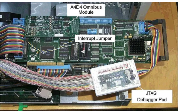
The two galvos are driven by analog waveforms generated by a second, 160 MHz M62
DSP card using DACs on an A4D4 analog I/O module. Raw galvo position data are
digitised by ADCs on the A4D4. Galvanometer position updates are synchronised to the
acquisition of range samples by using a hardware interrupt signal. The VCLK_INT
interrupt is presented to the ‘galvo’ M62 card through an unpopulated Omnibus interface
site (Site 1). It connects directly to an interrupt input, ExtInt2 available on JP23, pin 29
Fig. 12.
Figure 12. Configuring the VCLK_INT Interrupt.
The external VCLK_INT interrupt is used to synchronise the Galvo M62 DSP. It is hardwired through an
unused Omnibus site as shown in the photo.
The Q67 is the main DSP system processor Fig. 11. All four onboard DSPs are
interconnected via dedicated, high-speed, bi-directional, 32-bit data links (“FIFOLinks”).
In addition, three off-board data links (“FIFOPorts”) provide similar connections to the
two M62 cards, however the FIFOPorts are limited to 16-bit transfers. One DSP on the
Q67 is connected to the PCI bus to support communications with the host PC, but the
other three are fully embedded. In this system, one FIFOPort remains uncommitted and
is available for system expansion. Each M62 card has direct access to the PCI bus to
support user interaction. This will be described in a later section that discusses system
software.
4.3
The Prototype Laser Scanner
The prototype sensor head (Fig. 9) contains the electro-optical and electro-mechanical
components. A fibre-optic cable carries the light from an external 10 mW laser source to
the sensor head. The X and Y scanning mirrors are driven by General Scanning model
G120DT and G325DT galvanometers respectively. These galvo driven mirrors provide
the X-Y optical deflection for both the outgoing laser beam and the returning reflected
light. A photodetector consisting of an EG&G Reticon RL0128TB 128-element CCD
device is used for light capture.
4.4
The Scanner PC Interface Electronics
The prototype scanner head contains only electro-optics and electro-mechanics; no
computer interface is provided. The external hardware that is used to interface the head to
a computer is described in this section. This includes the clock generation logic, the
camera control card and the synchronisation logic. The latter is used to synchronise raw
range data acquisition (CCD video signal) with the laser pointing (galvanometer
positioning). Hardware interconnections are also summarised in this section.
Clock Generation Card
The clock generation card, Fig. 13 produces both the CCD clock used to drive the CCD
device and the “VOXEL CLOCK” which sets the voxel sample rate. The CCD clock
must be allowed to run continuously to avoid saturating the CCD device. The CCD clock
is derived from a 10 MHz crystal controlled oscillator, X1, not a 20 MHz oscillator as
shown in the drawing. JP1 is set to position 1-2 to select a 5 MHz CCD clock output. U2
generates the VOXEL CLOCK. Jumper JP4 is installed to produce a VOXEL CLOCK
Figure 13. The Clock Generation Card.
A 10 MHz master oscillator (X1) is divided by U1A to derive a 5 MHz CCD clock (JP1-2). The VOXEL
CLOCK signal (U2-14), which is derived from the CCD clock by U2, is used to set the sample rate of the
scanner. Both signals are driven off-board using RS422 drivers (U3A/B) and are available from headers
JP2 and JP3.
Camera Control Card
Fig. 14 shows an original drawing for the Camera Control Card. A number of
modifications have been made for this project and will be described here. For our
purposes, the main role of this card is to provide the initial analog preprocessing of the
raw CCD video signal. However both the CCD clock and the VOXEL CLOCK from the
clock generation card are interfaced to this card via J18 and J35. The clock signals are
handled by U15, DS8922 differential receivers/drivers.
The raw CCD video signal is presented to SMA connector J25. Here it is lowpass filtered
and amplified by U16, an AD818AN op amp. The filter characteristics are determined by
new values for C24 (82pf) and R16 (5.1k) and yield a lowpass cut-off frequency of about
380 kHz and a voltage gain of about 34 dB. R17 has been replaced by a 100-ohm resistor.
The filtered video output is available from SMA connector, J23.
Commercial higher order LC lowpass filters can be inserted ahead of the inverting input
to U16. Typically these filters require 50-ohm terminations and so will affect the gain of
the preamplifier.
Synchronisation Logic
Fig. 15 shows the synchronisation logic which is used to provide exact control of
CCD_CLK, the clock used for sampling of the CCD signal by the ADC on the A4D1
Omnibus Module. This clock is controlled by software to allow exact synchronisation
with the galvo waveforms. The logic accepts as inputs the CCD clock, the VOXEL
CLOCK and the software generated FIFO_EN signal from the galvo M62 DSP. It
generates CCD_CLK, which clocks the A4D1 ADC and strobes raw data into the FIFO
buffer. This logic also handles the free-running VCLK_INT signal, which is used to
interrupt the galvo M62 DSP at the voxel sample rate. VCLK_INT interrupts the M62
galvo controller continuously even if the galvo controller is idling and waveforms are not
being generated. DS8922 differential receivers/drivers, U1 are used to receive the input
clocks, and SN75121 line drivers, U4 are used to drive the outputs.
When a command is issued to initiate a scan, the galvo M62 will asynchronously assert
FIFO_EN and will then begin to step the galvos. FIFO_EN is used to enable CCD_CLK.
However for the scanner to produce meaningful data, startup of the CCD_CLK must
always coincide with the VOXEL CLOCK, i.e. both laser position control and CCD
sampling must be synchronised Fig. 16. The synchronising logic delays the start of the
CCD_CLK until the arrival of the next VOXEL CLOCK. CCD_CLK then remains
synchronised for the duration of the scan.
U3 is used to synchronise the generation of CCD_CLK. Its output, U3-5 is asserted on
the next occurrence of the VOXEL_CLOCK if FIFO_EN has also been asserted. It
remains asserted until a VOXEL_CLOCK occurs in which FIFO_EN has been negated.
This signal is used to gate the free-running CCD clock in U4B to produce the
synchronised CCD_CLK output. This synchronisation guarantees that the ADC and the
FIFO always capture a full complement of samples and that these samples are properly
aligned with the galvo scans.
A number of discrete synchronising signals are also generated by the galvo M62 board
using JP14, the Digital I/O connector. These signals include the FIFO_EN signal
described earlier as well as the HYNC and VSYNC (horizontal/vertical synch) signals.
Figure 15. Synchronisation Logic.
This logic accepts the clock signals from the camera control card and the asynchronous FIFO_EN signal
from the M62 DSP. It generates VCLK_INT, which by interrupting the galvo M62 sets the system sample
rate, and CCD_CLK, which synchronously clocks raw CCD data into the ADC and FIFO.
Hardware Interconnections
Interconnections between the M62 DSP cards and the external logic consist of prototype
cabling supplied by the DSP board manufacturer
10. The M62 card uses industry standard
0.100” square double row 50-pin headers. Five 50-pin ribbon cables carry the signals to
outboard transition modules (Weidmuller, RI 50A), Fig. 8. No attempt has been made to
simplify this wiring. The five cables consist of three from the galvo M62 and two from
the peak M62 card. The “Galvo cables” include: the synchronisation signals from the
DIO interface via JP14, the VOXEL CLOCK interrupt signal on JP22, and the analog
input/output signals from the A4D4 Omnibus module via JP18. The “Peak cables”
include the CCD signals for the A4D1 Omnibus module on JP18, and the DIO signals
from the DIO interface via JP14. A number of DIO signals on both the Galvo M62 and
the Peak M62 have been allocated for test purposes. These allow timing measurements of
peak detector and galvo controller performance.
Figure 16. Synchroniser – Timing Diagram.
FIFO_EN is asserted asynchronously by the galvo M62 DSP. It is synchronised to the VOXEL_CLOCK
and then used to gate the free-running CCD clock to produce the synchronised CCD_CLK. This guarantees
that for each range sample, an exact number of raw CCD data samples are digitised by the ADC.
5. Software Configuration
3DMD has been implemented using an embedded array of DSPs based on three PCI bus
circuit boards installed in a desktop PC. The DSPs are used to implement the 3D laser
scanner and the motion detector while the PC is used for higher-level functions such as
for data handling and as a user interface.
The DSP system has been divided into two major components: the two “front end”
controllers, which manage the galvanometers and the CCD range data, and the main
processor block, which performs higher-level processing such as for motion detection,
and command and data handling.
There were two main design goals in the development of MDSP, the DSP architecture
7:
to produce a system that can meet the real-time constraints imposed by the 3D laser
scanner, and to develop a scalable system that can be easily adjusted in the future to
handle expanding requirements.
To meet these needs, we chose to implement the system software with a commercial
real-time operating system (RTOS), MQX produced by Precise Software Technologies Inc.
8This section describes the software structure that has been built. The design supports
modularity through the use of multitasking and multiprocessing. Because of hardware
constraints, we had to use a message communication model rather than a shared memory
model; message passing is used for intertask synchronisation and communication.
This section will begin with a brief outline of the main characteristics of the RTOS and
will then present an overview of the system software. We will then describe the front-end
DSP components that operate outside the RTOS abstraction and then discuss in some
detail the RTOS task structure used to implement the high-level DSP system. We will
follow this with short summaries of the messages that are used, and of the task creation
sequence used at system startup. We will conclude this section with a description of the
PC-based user interface, which has been written in Visual Basic.
5.1
General Features of the MQX Real-time Operating System
A multitasking RTOS facilitates the implementation of a complex system by allowing the
software functionality to be partitioned and expressed as individual tasks. The RTOS
provides mechanisms that support communications and synchronisation between the
tasks. The additional ability to extend this multitasking abstraction across multiple
processors adds considerable flexibility since this not only allows true parallelism to be
achieved but also permits the number of processors in the system to be adjusted as the
need arises. This is the approach used for 3DMD.
For this project we selected MQX from Precise Software Technologies Inc. We made a
number of fundamental design choices at the beginning of the project. For example, we
chose to use pre-emptive task scheduling rather than round-robin time slicing, and we
chose message passing over semaphores or mutexes for intertask synchronisation. We
chose message passing (Feb. 2001) because it was the only communications mechanism
provided by MQX for use in multiprocessor environments. It is a more general solution,
allowing us if necessary to easily reconfigure the software by moving tasks from
processor to processor without limitation.
In MQX, tasks are assigned static priorities at compile time and may be created or
destroyed dynamically at runtime. Task queues are used extensively by MQX. The
“ready queue” maintains a prioritised list of tasks (first in, first out at each task priority
level) which determines which task will be dispatched on the next pre-emption. In MQX,
a task can be either running (the “Active” task), waiting to run but queued on the ready
queue, or “blocked” (queued on some other queue). Tasks are added to or removed from
the ready queue by the operating system kernel in response to events (creation of a task,
arrival of a message, etc.) or by explicit function calls.
task and adjusting the task “ready queue” for that processor. At the conclusion of this
pre-emption, the highest priority task that is ready to run will be dispatched.
A number of system calls are provided in MQX to implement message passing. One of
these, _msgq_receive() uses “blocking semantics” whereby the calling task will “block”,
i.e. be suspended from execution, until the arrival of a message. Indefinite blocking can
be avoided by using a timeout. Other system calls for example allow a message to be sent
to a destination queue or queues, or allow a task to poll a queue for a message without
blocking. These calls allow considerable flexibility in configuring an application.
Some overhead is required in preparation to sending a message. For example, a message
pool consisting essentially of blank messages must be created by the task before any
messages are to be sent. Before sending a message, the source task must first fetch a
blank message from the message pool and then fill in the necessary fields (source and
destination addresses, size, data etc.). Finally, after receiving the message, the destination
task must deallocate the message and return it to the message pool to avoid a memory
leak. Message contents are user defined.
Interprocessor communications (IPC) between tasks on different processors is more
complex and more expensive than for the single processor case. For MDSP, the low-level
communications for IPC makes use of the FIFOLinks that interconnect all of the C6x
DSPs on the Q67 processor board (Section 4.3). Because MQX had not been ported to
this hardware, it was necessary for us to fully develop the IPC mechanism for this
system. IPC is fully transparent to the user; messages destined for tasks on remote
processors and those destined for tasks on the local processor only differ in the
destination field of the message.
MQX uses a routing mechanism for multiprocessor message passing. The user must
construct a static routing table for each processor. Each entry in the table corresponds to
a mapping between the intended destination processor and a local queue which will
trigger the IPC mechanism. For example, all messages intended for message queues on a
remote processor “A” will be sent to a local message queue, for example “_id_A_q”. This
will trigger the IPC mechanism that will result in the message being transferred to the
destination queue on processor “A”. In an arbitrarily large system where processors are
not fully interconnected, the routing table allows the user to define message routing that
may involve hops between multiple processors before the message is finally delivered to
its destination. In comparison to local message passing, there is a performance penalty
associated with message passing to remote processors. The cost of this penalty is directly
related to the complexity of the message route. Software design for any multiprocessor
real-time system must pay careful attention to the fixed cost of message passing, and
design the task configuration accordingly. Task to task intercommunication should be a
deciding factor in determining task proximity.
For real-time systems, efficient interrupt handling is essential. To address this, MQX
provides an interrupt handling mechanism called a “notifier”. A notifier can be viewed as
a high-level interrupt service routine (ISR) which possesses some characteristics of MQX
tasks. Typically, a notifier is installed very much like an interrupt service routine and is
activated by a first level interrupt handler whenever that interrupt is asserted. Once
active, the notifier usually clears the interrupt and fetches any volatile data. An important
feature of a notifier is that it can also call any non-blocking MQX function. For example,
it can send a message to a task that is currently blocked waiting to respond to this
interrupt. This provides a simple and efficient way to synchronise task behaviour with
external events.
We have measured the typical latency between the arrival of an interrupt and execution of
an interrupt service routine on a 160 MHz C6201 to be about 1.0
µ
s. For 3DMD,
notifiers are used on the Q67 for handling incoming data on FIFOPorts from the peak and
galvo DSPs. These notifiers each trigger a task. The latency for the dispatch of the tasks
cannot be measured directly however we estimate that it would be about 5 to 10
µ
s.
5.2
Overview of the System Software
The software for 3DMD consists of the PC-based user interface, and the real-time MDSP
software, most of which runs on MQX. The PC-based user interface has been
implemented with Visual Basic 6.0 and provides a number of forms to support user
interaction (see Section 3).
Communication between the PC-based user interface and the embedded target DSP is
based on an ActiveX control called DSPComponent
11, supplied by Innovative
Integration, the manufacturer of the DSP boards. DSPComponent can be used directly by
Visual Basic applications. It does however require a complementary board support DLL
from the board manufacturer. DSPComponent works in conjunction with a library of
functions which run on the DSP target. Together, they support communications between
the PC and the target using mailboxes and interrupts. This will be outlined in more detail
in the next Section.
MDSP exploits the multitasking and multiprocessing capabilities of MQX. Early
measurements of IPC performance played an important role in the design of the system
software. Preliminary performance measurements indicated that message traffic between
“Peak M62”, the DSP that handles the raw CCD video data (Fig. 11) and Q67, the main
DSP board, would exceed the IPC capabilities. To avoid this limitation, we decided to
remove Peak M62 from the RTOS abstraction, in effect defining it as a “custom
peripheral”. The same decision was taken for the “Galvo DSP” which controls the
scanning galvanometers. Both DSPs communicate with the Q67, the main DSP system,
5.3
Host PC and Embedded DSP Target Communications
DSPComponent was introduced in Section 5.2. It provides an ActiveX component, which
can be integrated directly into a Visual Basic application, and which supports runtime
communications between the Visual Basic program and the target DSP system.
DSPComponent includes a number of properties, methods and events. A set of functions
must run on the target DSP to complement this functionality. The board manufacturer
provides these functions in the form of a runtime library.
DSPComponent includes a bi-directional interrupt mechanism. A target DSP can call
mailbox_interrupt() to trigger an interrupt on the host PC. The incoming interrupt at the
PC will trigger an “OnInterrupt” event that automatically activates a user-written event
handler object. The event handler will use the “InterruptAcknowledge” method to handle
and clear the interrupt and read any associated data. Similar methods exist to transfer
interrupts in the opposite direction.
DSPComponent also uses mailboxes for exchanging data between the host PC and the
target DSP. The target DSP calls write_mailbox() and read_mailbox() to transfer data to
or from a mailbox while the host PC uses the “Mailbox” property for the same purpose.
Other properties or functions are provided to allow the host or target to check the status
of a mailbox for polling purposes.
5.4
The Peak Detector and Galvo Control DSPs
For efficiency, DSPs have been dedicated to two critical front-end processes: CCD data
handling, and galvanometer control. These DSPs are treated as custom peripherals that lie
outside the multitasking abstraction. The Peak DSP handles the raw CCD data and
extracts raw range and intensity data corresponding to each sample point. These data are
fed continuously to the main DSP system. The Galvo DSP manages waveform generation
and returns galvo position data to the main DSP system for further processing.
While the system is actively scanning, analog CCD data are generated continuously.
These data are digitised by an ADC onboard the A4D1 Omnibus module on the Peak
M62 and are stored in a FIFO buffer, Fig. 11. When the FIFO becomes half full, an
interrupt is triggered to the Peak M62 DSP. The DSP interrupt service routine transfers
these data using direct memory access (DMA) to local DSP memory. It then executes a
peak detection algorithm
9which computes not only the position of the peak with
sub-pixel resolution but also the corresponding intensity of the peak. The peak position
represents the CCD element actually illuminated by the returned laser spot and is related
through triangulation to the range to the target. Range and intensity data are then
transferred to the Q67 via a FIFOPort.
Both front-end DSPs are heavily loaded. We have measured the 200 MHz Peak M62
DSP load to be about 69% when the CCD is clocked at 5 MHz. This does not allow
sufficient time to implement message passing to tasks on the main DSP board. For this
reason, this software runs independently and simply passes the data to the main DSP via a
FIFOPort. The peak DSP is a free-running system, it requires no input commands to
operate.
The 160 MHz Galvo DSP is integrated into the system in a similar manner. For the
3DMD application, it is running at about 97% capacity. Unlike the Peak DSP, the Galvo
DSP fetches incoming commands to handle initialisation and runtime waveform
adjustments. The Galvo DSP also returns position data for the two galvos to the main
DSP using a FIFOPort.
A FIFOPort buffers data received by the main DSP, either from the Peak DSP or the
Galvo DSP. When a FIFOPort buffer becomes half full, an interrupt is generated to the
destination Q67 DSP which then transfers the incoming data. This is done within the
multitasking abstraction using notifiers.
5.5
3DMD System Task Configuration
The application software, which runs under MQX, has been partitioned into tasks, Fig.
17. Initialisation and task creation will be described in Section 5.7.
Idle State
After initialisation and the creation of all tasks, the system enters an ‘idle’ state awaiting
input commands from the user interface. The Galvo DSP continuously responds to and
discards incoming VOXEL_CLOCK interrupts since no scan is active. The Peak DSP
simply idles.
Parameter Setup
From the idle state, the user has complete access to all system parameters. The user can
define and adjust the scanning waveforms, change the motion detection parameters, and
start and stop a scan.
User requests to define or adjust a scanning waveform are handled by the
User_Interface_Task() on DSP_A. The PC-based graphical user interface formats all
such requests into commands which are sent directly to the DSP system via the mailbox
Figure 17. The Task and Message Structure for the MQX-based ‘Q67’ Multiprocessor DSP System.
Five tasks distributed across three DSPs are used in the implementation of the 3DMD prototype. Two
additional dedicated DSPs provide low-level control and processing for CCD data acquisition and
galvanometer control. These ‘external’ DSPs feed data to the main board using ‘FIFOPort’ data
communication links where interrupt triggered ‘notifiers’ handle the incoming data. The
User_Interface_Task() and the Display_Driver_Task() communicate with the PC-based user interface using
the PCI bus on the PC’s backplane.
The Galvo_Control_Task() is normally blocked, waiting to receive a message from the
User_Interface_Task(). An incoming message will unblock the task which will then
proceed to interpret the command. The Galvo_Control_Task() will then generate a
low-level command directly to the Galvo DSP and after the transfer is complete, will send an
acknowledgement message to the User_Interface_Task() to complete the message
handshake. On receipt of the acknowledgement message, the User_Interface_Task()
resumes polling for the next incoming user command.
The repertoire of commands for the galvo control DSP include: initialise galvo, start
galvo, stop galvo, define waveform, change amplitude of current waveform, change
phase of current waveform, change offset of current waveform and select another
waveform. A total of 16 waveforms can be defined and stored by the Galvo DSP.
Waveforms can be changed dynamically at runtime by simply selecting its wave index.
Active Scanning
In response to a user request to start a scan, the Peak_Data_Task() initialises its internal
data structures and resynchronises its communications with the Peak DSP. Also, the
Galvo_Control_Task() issues a START_GALVO command message to the Galvo DSP.
This command is interpreted by the DSP which then begins to generate the two scanning
waveforms. In addition, the Galvo DSP enables the generation of CCD range and
intensity data by asserting the FIFO_EN signal to the synchronisation logic (Section 4.4
and Fig. 11). The range and intensity data are now transferred to the FIFOPort that
connects the Peak DSP to the main Q67 DSP board.
As the Q67 FIFOPort fills, it generates interrupts that are handled by the
Peak_Data_Notifier(). With each interrupt the Peak_Data_Notifier() uses a DMA transfer
to move the contents of the FIFOPort to a local buffer that is managed by the
Peak_Data_Task(). This local buffer contains the raw range and intensity data that are
used by the motion detector.
Motion Detector
The motion detector not only processes the range data for the detection of objects in
motion but also prepares them for transfer to the PC for real-time display. The
Motion_Detect_Task() is implemented as a loop. At the top, the task sends a message to
the Peak_Data_Notifier(), requesting the latest complete line of range data. In its loop,
the notifier polls for an incoming message from the Motion_Detect_Task(). (By
definition, a notifier cannot call blocking functions, since this is inconsistent with proper
design of interrupt handlers.) If a request message is found, the notifier responds by
sending a message containing a ‘structure pointer’ to the Motion_Detect_Task(). The
structure contains the information which allows the Motion_Detect_Task() to directly
access the latest acquired line of range data.
The motion detection algorithm (Section 2.2) is then executed. The ‘index’ (position
along a scan line) and ‘value’ (departure from average position) of any points that surpass
some threshold, are stored in a message buffer that can be sent to the
Display_Driver_Task(). The Motion_Detect_Task() will poll for a message from the
Display_Driver_Task(). If a request message is available, then the message is sent and
execution returns to the top of the loop. Note that if the Display_Driver_Task() has not
reported with a new message, the Motion_Detect_Task() continues without interruption.
This means that motion detection is continuous, and independent of the performance of
the display system.
Display_Driver_Task() requests data from both the Motion_Detect_Task() and the from
the Galvo_Data_Notifier(). It receives all of these data and combines them into a single
data structure, which contains points in motion, their intensity (value) and their positions
(X- and Y-galvanometer positions). These data are all sent to the display application on
the PC.
The galvo position data are derived directly from the galvo controller’s position sensors.
Ideally, the waveform displayed on the user interface should be identical to the actual
laser scan seen on the target. However, we have found that the displayed waveform is
slightly distorted (see Section 2.3).
An alternate implementation had been used earlier in which the galvo positions were
computed based on the index of the sample points. Since the waveforms are
predetermined, it is easy to compute the corresponding X-Y co-ordinates for each point.
However, this method does require careful calibration. For any set of scan parameters, a
fixed delay will exist between the generated galvo waveform drive voltages and the
actual galvo positions. These phase delays must be measured carefully and included in
the calculation of the final position of each sample.
Comment
It should be clear from the above that the use of multitasking with message passing yields
a very flexible architecture. In general, communications between software objects (tasks)
can be easily configured regardless of which processors are actually involved. Of course,
careful placement of tasks is required to meet performance needs. For example, the
assignment of the Motion_Detect_Task() and the Peak_Data_Task() to the same
processor was done to give the motion detection algorithm direct access to the raw range
data. This avoids unnecessary and expensive interprocessor data transfers.
5.6
Summary of System-wide Message Passing
User defined messages are used throughout this application. Each message type is
defined as a dedicated data structure. For example, the message type used for messages
sent by the User_Interface_Task() to the Galvo_Control_Task() are of type
GALVO_CMD_MESSAGE_STRUCT.
t y p e d e f v o la t ile s t r u ct g a lv o _ cm d _ m e s s a g e {
MES S AGE_ HEADER_ S TRUCT HEADER;
u in t _ 1 6 GALVO_ CMD;
u in t _ 1 6 WAVE_ INDEX;
WAVEFORM_ DEFINE_ S TRUCT WAVEFORM_ DEF;