Building a Computer Poker Agent with Emphasis
on Opponent Modeling
by
Jian
Huang
B.S. Computer ScienceMassachusetts Institute of Technology, 2011
Submitted to the Department of Electrical Engineering and Computer Science In partial fulfillment of the requirements for the degree of
Master of Engineering in Electrical Engineering and Computer Science At the
MASSACHUSETTS INSTITUTE OF TECHNOLOGY September 2012
02012 Jian Huang. All rights reserved.
The author hereby grants to MIT permission to reproduce and to distribute publicly paper and electronic copies of this thesis document in whole or in part
in any medium now known or hereafter created.
A~~g~E$
Signature of Author:
Department of Electrical
- A
Engineering and Computer Science August 29, 2012 Certified by:
Professor of
teslie P. Kaelbling Computer Science and Engineering Thesis Supervisor Accepted by:
Prof. Dennis M. Freeman Chairman, Masters of Engineering Thesis Committee
Building a Computer Poker Agent with Emphasis
on Opponent Modeling
by Jian Huang
Submitted to the Department of Electrical Engineering and Computer Science On August 25, 2012 in Partial Fulfillment of the
Requirements for the Degree of
Master of Engineering in Electrical Engineering and Computer Science
ABSTRACT
In this thesis, we present a computer agent for the game of no-limit Texas Hold'em Poker for two players. Poker is a partially observable, stochastic, multi-agent, sequential game. This combination of characteristics makes it a very challenging game to master for both human and computer players. We explore this problem from an opponent modeling perspective, using data mining to build a database of player styles that allows our agent to quickly model the strategy of any new opponent. The opponent model is then used to develop a robust counter strategy. A simpler version of this agent modified for a three player game was able to win the 2011 MIT Poker Bot Competition.
Thesis Supervisor: Leslie P. Kaelbling
Acknowledgements
First I want to thank my supervisor, Leslie Kaelbling, for giving me the opportunity to work with her and others in LIS. She has given me great feedback and directed me to people whom I was able to work with.
Next, I give my thanks to Frans Oliehoek who has been mentoring me throughout the project, even after moving to Amsterdam. The reading materials and guidance from him have been very helpful.
I want to thank Chris Amato who joined us later in the project. I appreciate the wonderful feedbacks and suggestions from him, and best wishes to his newborn son.
Also, thanks David Shi for printing and hand in this thesis for me while I am off campus! Finally, I want to thank my family for their support and my friends for the great times we've had together.
Contents
1 Introduction 9 1.1 M otivation ... 10 1.1.1 W hy Gam es?... . . . 10 1.1.2 W hy Poker?... 11 1.2 Thesis Contribution ... 12 1.3 Thesis Organization ... 13 2 Background 15 2.1 Rules of No-Limit Texas Hold'em ... 152.2 Game Theoretic Overview ... 17
2.2.1 Strategy ... 19 2.2.2 Nash-Equilibrium ... 20 2.2.3 Best Response... 20 2.3 Related W ork ... 21 3 Opponent Modeling 25 3.1 Abstractions ... 26 3.1.1 Hand Strength ... 26 3.1.2 Action Sequence ... 28
3.2 Generalizing Across Information Sets ... 30
3.2.1 Data Mining ... 31
3.2.2 Strategy Reconstruction ... 31
3.2.3 Estimating Strategy of New Opponents ... 36
4 Decision Making 39 4.1 Opponent Hole Card Distribution ... 39
4.2 Estimating Expected Return ... 40
4.2.1 Uniformly Random Action Selection ... 41
4.2.2 Self-Model Action Selection ... 41
4.3 Calculating Strategy using Expected Returns ... 42
5 Results 43 5.1 D uplicate Poker ... 43
5.2 Experim ents ... 44
5.3 M IT Poker Competition ... 46
6 Conclusion and Future Work 49 6.1 C onclusion ... 49
6.2 Future W ork ... 50
6.2.1 Improving Data Mining ... 50
List of Figures and Tables
Figure 1.1 shows the high-level model of the computer agent and how it interacts with the environm ent ... 12 Table 1.1 shows types of 5-card hands for Texas Hold'em poker from strongest to weakest . .. 17 Figure 2.1 shows a partial tree representing a two-player game of poker ... 18 Table 3.1 examples of action sequences mapping to buckets ... 29 Figure 3.1 shows an example of the probability of calling or raising with respect to hand strength when d = <0.3, 0.3, 0.2, 0.2> ... 32 Figure 3.2 shows graphs of action distributions vs. hand strength ... 34 Figure 3.3 shows action probabilities vs. hand strength individually ... 35 Figure 4.1 shows how the agent updates the probability distribution of opponent's hole cards . 40 Table 5.1 shows the results from matches played between pairs of computer agents ... 44 Figure 5.1 graphs the net profit of Random as the match against Self-Model progressed ... 45 Figure 6.1 illustrates a visual representation of the balanced strategy and shows how it is
Chapter 1
Introduction
Playing games is something that most people have done at some point in their lives. Whether it is a board game, card game, or video game, we generally begin by learning the rules of the game, and then we gradually improving in skill level as we gain more experience. In competitive games where players are pitted against one another, the more skillful players come on top more often than not.
Now what if we want to create computer programs that could play these games? They will essentially need to make decisions given some information or knowledge just like human players. While it is possible to create rule-based computer agents using expert knowledge of humans, this approach is often cumbersome and inflexible, especially in games such as poker where opponents' playing styles play a large role in the decision making.
In this thesis, we will study opponent modeling in the game of two-player no-limit Texas Hold'em poker and build a computer agent using an opponent modeling approach.
1.1
Motivation
1.1.1 Why Games?
Artificial Intelligence research involving classic games has been around since as early as the advent of computers. Chess, Checkers, and Othello are some of the earliest games to be studied. As of today, the best chess programs, having estimated elo ratings of over
3200, far surpass the current human Chess world champion Magnus Carlsen's 2837 rating[2][14]. Checkers has been solved for perfect play in 2007[10]. Starting from
around the past decade, poker has been receiving increasing attention by researchers as the game experienced a dramatic boom in popularity.
Games are usually a form of entertainment, but why should anyone devote so much time toward developing AIs for them? Well, games are all about making decisions -potentially under time constraints - using some set of knowledge or information. It's just
like what people, companies, and governments do every day in the real world, from trading stocks to setting prices of new products. When different choices are available there are of course different outcomes, some better than others. Therefore, we want to
study decision making in classic games to be able to apply similar techniques to problems in the real world.
1.1.2 Why Poker?
Poker, a game that is often said to be easy to learn but hard to master, has a number of defining characteristics that makes it different from some of the previously mentioned games:
1. Poker is an imperfect information game, meaning players cannot observe the entire state of the game. Each player can see the cards they are holding, but not the ones in the opponent's hand.
2. Poker is stochastic, meaning the same action performed in one game state can probabilistically transition into a number of different game states. Unlike in chess where each move can only have a single fixed outcome, in poker, future
community cards are random.
3. Poker has varying levels of success in each game. In chess, it does not matter if you reach checkmate with all your pieces remaining or only one. In poker, you want to win as much chips from the opponent as possible.
These properties of poker are also shared by most real world problems. Nobody can possess every bit of information available, nor can anyone predict the future with one hundred percent certainty. Outcomes are rarely confined to perfect success or failure, but rather somewhere in between. While the addition of these properties is a better reflection of reality, it also makes creating a computer poker agent a challenging and interesting problem for research. A number of groups in the research community have been actively
tackling this problem, and there are also computer poker competitions such as the one held annually at the annual AAAI conference to showcase their efforts.
1.2 Thesis Contribution and Focus
Agent
Decision making Belief Opponent ModelH
Environment
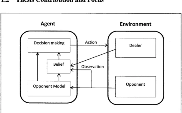
Action Observation Dealer OpponentFigure 1.1 shows the high-level model of the computer agent and how it interacts with the environment.
This thesis focuses on creating a computer agent for poker from an opponent modeling perspective. The high level picture of our agent is described in Figure 1.1. The agent has an opponent model that is updated when there is an observation of opponent action. The belief, which is a probability distribution over state spaces, is updated with the help of the opponent model after any observation from the environment. Both the opponent model and belief contribute to the agent's decision making component which uses a simulation
The opponent modeling and decision making algorithms are formulated in collaboration with Frans Oliehoek and Chris Amato. The author implemented the computer agent and poker engine on which to test the agent and also performed the experiments shown near the end of this thesis.
1.3
Thesis Organization
Chapter 2 gives an overview of poker and presents some of the existing computer poker agents. Chapter 3 describes the method we use to model the opponent's strategy,
including game state abstractions and inference through data mining. Chapter 4 discusses the decision making part of the agent and how we make use of the opponent model and simulation techniques to facilitate this process. Chapter 5 shows the performance of the agent when running against a number of benchmark opponents as well as comparisons of algorithms used in different versions of the agent.
Chapter 2
Background
2.1
Rules of No-Limit Texas Hold'em
There are many variations of poker and different formats of competition, such as tournaments or cash games. The most popular variation is Texas Hold'em, and in this thesis we will focus on two-player No-Limit Texas Hold'em.
Each player starts with a stack of chips that they can use to make bets. The goal is to win chips from the opponent through a number of short games. The game begins when both players place forced bets called blinds. One player called the dealer will be the small blind, and the other player will be the big blind which is generally double the amount of the small blind.
Next, two cards called hole cards, seen only by the player holding them, will be dealt from a standard 52-card deck to each player, followed by a round of betting where players take turns making actions. The first round of betting starts with the dealer. During each player's turn, he has the three types of actions to choose from.
If a playerfolds, he forfeits the hand and all chips that were bet in this game goes to the other player immediately.
If a player checks or calls, he will match the amount the opponent has bet. If the opponent bet nothing, the action is a check, otherwise it is a call. If the caller has fewer chips than the amount raised, then he will simply bet all he has and the unmatched chips will be returned to the raiser.
If a player bets or raises, he increases the amount to be wagered, forcing the opponent to call or raise again if he does not want to give up the hand. The amount that can be raised in a limit game is always a single fixed amount of either one or two big blinds, and in a no-limit game is any amount between the big blind and one's entire chip stack. If the opponent has made a bet or raise in the current round, the minimum raise amount is then at least the amount the opponent has raised by. For example, if player A bets 20 chips and player B raises to 70 chips, then if player A wants to raise again, the amount must be at least 120 chips.
A round of betting ends when both players have made at least one action and the last action is a check or call. Essentially the players can raise back and forth as many times as they like until one player has bet his entire chip stack or calls. However, in reality raises rarely occur more than 3 or 4 times in one round.
After the first round of betting, 3 community cards called the flop that both players share are dealt from the same deck. This is followed by another round of betting, this time, starting with the player who is not the dealer. Then 1 community card called the
turn is dealt with another round of betting, and finally the last community card called the river is dealt with the last round of betting.
If neither player has folded after the last round of betting, then they will go to the showdown where players reveal their hole cards and each will look for the best 5 card combination they can make using any combination of their 2 hole cards and the 5 community cards. The player with the stronger 5 card combination wins all of the chips that were wagered in this game, called the pot. If the card strengths are the same, then they share the pot.
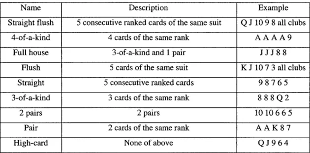
Strengths of 5 card combinations are listed in Table 1.1 below.
Name Description Example
Straight flush 5 consecutive ranked cards of the same suit
Q J 10 9 8 all clubs
4-of-a-kind 4 cards of the same rank A A A A 9
Full house 3-of-a-kind and 1 pair J J J 8 8
Flush 5 cards of the same suit K J 10 7 3 all clubs
Straight 5 consecutive ranked cards 9 8 7 6 5
3-of-a-kind 3 cards of the same rank 8 8 8
Q 2
2 pairs 2 pairs 1010665
Pair 2 cards of the same rank AAK87
High-card None of above
Q
J 9 6 4Table 1.1 shows types of 5-card hands for Texas Hold'em poker from strongest to weakest. Within each category, the ranks of the cards will further decide their strengths. For example KKK32 is stronger than JJJ94, and 88Q43 is stronger than 88J96. Ties are therefore fairly uncommon.
2.2
Game Theoretic Overview
Two-player poker can be modeled as a zero-sum game. The representation, or extensive form, of the game is a tree, where nodes are game states and directed edges are transitions.
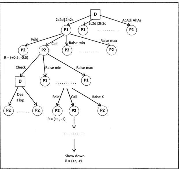
Figure 2.1 shows a partial tree of the game that shows some of the important features. There are two types of nodes in the tree, decision nodes that transitions based on action from players and dealer nodes that make stochastic transitions when cards are dealt.
D
2c2dj2h2s c2dj23c AcAdjAhAs
Pi Pi ... Pi
Fold Call Raise min Raise max P2 P2 ... P
R = (+0.5, -0.5)
Check Raise min Raise max
D Pi Pi
Deal Fold Call
Raise X Flop P2 ... P2 P2 P2 P2 R = (+1, -1) Show down R=(+r,-r)
Figure 2.1 shows a partial tree representing a two-player game of poker. Many of the nodes and transitions are omitted. The square nodes are the dealer nodes, and circle nodes are decision nodes for the players. The game begins with the root dealer node transitioning to player 1 through one of around 2 million hole card combinations. The players then take turns making actions. When a fold or show down occurs, the game ends and positive and negative rewards are given out.
Because poker is an imperfect information game, players do not get to see the entire game state whenever making an action. The part of the game state that the player can observe is called the information set, which includes his own hole cards, community cards, and previous actions - in other words, everything except the opponent's hole cards.
2.2.1 Strategy
We define a strategy as a mapping from any information set to a probability distribution over legal actions. We use a probability distribution over actions because in imperfect information games, these mixed strategies are more robust than pure strategies that maps information sets to fixed single actions. A simple example to illustrate this claim with the
game of Rock, Paper, Scissors is that the strategy of always choosing Rock is much easier to recognize and exploit than a strategy that chooses the three actions uniformly at random. Now tying strategies back to our extensive form game, notice that to a player,
many of the nodes in the tree have the same information set due to the hidden opponent hole cards. The number of information sets is actually much lower than the number of game states, and from a player's perspective, he could very well reduce the game tree by ignoring opponent's hole cards. The question now is what would be the best strategy for poker? There are two ways to look at this problem.
2.2.2
Nash-Equilibrium
First we will define the Nash-Equilibrium for a two-player zero-sum game.
Definition 2.1 Let -i be the strategy of player i. Let Tji be the strategy of player i's opponent. Also let the expected return of strategy ni be E(i, m-.). Then 7T* = (rI, 7T2) is a Nash-Equilibrium if and only if:
Vi' , E(t1i,m.i) > E(un', Tg) for i = 1,2
In other words, if each player is using a strategy such that changing it will not provide more expected return against the opponent's current strategy, then it is a
Nash-Equilibrium. An example of the Nash-Equilibrium for Rock, Paper, Scissors would be both players choosing the three actions uniformly at random.
For a zero-sum game like poker, at Nash-Equilibrium the two players can expect to tie in the long run. In reality, however, human players are not able to play so accurately and computer players can only play at an estimated equilibrium at best because finding an exact equilibrium for a problem of this enormous size is practically impossible.
2.2.3 Best Response
Suppose instead that we are playing against a terrible player who is using a static strategy, using the equilibrium strategy will certainly give us a positive expected return, but it's possible to do much better. We will define the best response strategy as follows.
Definition 2.2 Let it2 be the strategy of player 2, and let the expected return of strategy
ii be E(Tri, Tri). Then
4r
is the best response to 2 if and only if:V-n' ,
E(T', 72 ) > E(Ti, T2OThe best response is usually a pure strategy, meaning it itself is very exploitable. It is the best strategy to use against an opponent whose strategy is static and known perfectly, but that is also not a very realistic assumption.
2.3 Related Work
Currently the most popular approach to creating computer poker agents has been finding near-equilibrium strategies. As mentioned before, since it is impossible to obtain exact Nash-Equilibrium, a number of techniques are used to calculate near-equilibrium
strategies. Most competitive agents do so by using an abstraction algorithm to first reduce the number of game states and then using custom algorithms to solve the abstracted game for equilibrium [9]. This technique is used, in conjunction with a lossless information abstraction algorithm GameShrink, to solve a simpler version of the game called Rhode Island Hold'em Poker for the exact equilibrium [3]. However, for the much larger Texas Hold'em Poker, only lossy information abstractions can bring the game down to a manageable size.
A significant amount of work in poker Al has been done at the University of Alberta's Computer Poker Research Group (CPRG) led by Michael Bowling. They have developed
a number of poker agents over time for both Limit and No-Limit Texas Hold'em. Their current state of the art poker agents play a near-equilibrium strategy computed using an iterative algorithm called Counterfactual Regret Minimization (CFR). The idea behind CFR is essentially letting agents play against each other, adjusting their strategies after each hand to minimize how much more they would have earned by taking the best possible action, or regret [15].
This near-equilibrium approach appears to be one of the most promising techniques so far. In 2007, the poker agent Polaris played against world-class poker professionals in two-player Limit Texas Hold'em and won in a number of duplicate matches in the First Man-Machine Poker Championship [6]. Since then, the strength of Limit Hold'em agents has steadily increased and has reached or surpassed the human world champion level of play. However, No-Limit agents have not yet achieved that level due to the significant increase in the number of game states from having a much larger range of legal actions at each decision node.
Using a near-equilibrium strategy ensures that the agent cannot be exploited, but at the same time, it also limits itself from being able to fully exploit weaker opponents. In an environment consisting of mostly very strong players, playing a near-equilibrium strategy is a good idea as strong opponents rarely open themselves up to be exploited. However, not everyone is a strong player, and against weak opponents, there is no reason not to exploit them to a greater degree. After all, the objective of the game is not simply to win but to win as much as possible. Of course, the idea of exploitive counter-strategies in
model that learns the opponent's frequency of actions at every decision point and
attempts to exploit the opponent's strategy. While Vexbot would lose to some of the best equilibrium agents today, it could potentially be a better choice against weaker opponents [11].
The third approach is to use robust counterstrategies, where the agent would employ an exploitive strategy that limits its own exploitability. CPRG introduced the Restricted Nash Response algorithm for this approach. The algorithm computes a strategy that exploits the opponent as much as possible while having a lower bound on how much it would lose in the worst case scenario when the model of the opponent is inaccurate [1]. This approach is ideal for maximizing profits against unknown opponents. Our agent described in this thesis belongs to this third category. However instead of the technique above, we will explore the effectiveness of using a simulation-based approach to compute robust counterstrategies.
Chapter 3
Opponent Modeling
As stated earlier, we want to build a computer agent that implements a robust
counterstrategy against opponents. However before a counterstrategy can be built, we must first know the strategy of the opponent. We know that a strategy is a mapping from information sets to a probability distribution over legal actions, but let us define it more precisely.
Definition 3.1 Let I be the set of all information sets in a poker game. Let A be the set of all legal actions. Then a strategy is a function
r: I x A -> [0, 1]
Such that
Vi E I, Y (i, a) = 1
aEA
Now that we know how to describe a strategy, how do does the agent actually model the strategy of the opponent? No opponent will simply hand out his strategy on a piece of paper, so it must be learned through observations while playing. However, due to the
large number of game states and limited number of observations from the opponent, estimating the strategy proves to be rather challenging. We will describe the abstraction algorithm used to reduce the number of game states and data mining technique used to make inferences about little observed information sets in the opponent's strategy.
3.1
Abstractions
The number of information sets in Texas Hold'em is on the order of 1018 in limit Hold'em, and in no-limit the existence of additional action choices increases it to over
1050 in a game with starting stacks of 100 big blinds, making it impossible to store in memory without any compression.
To deal with this, abstractions must be used to greatly reduce the size without losing too much information. Abstractions essentially group together closely related information sets into a single one [12]. Since the information set in poker is composed of both cards and action sequences, we will focus on each one individually.
3.1.1 Hand Strength
A player can see at most 7 cards - 2 in his hand and 5 on the table. There are on the order
of 109 such combinations. To a player, the most important information about the cards is
the relative strength of his hole cards compared to all other possible hole cards, with respect to the community cards. Instead of keeping track of the individual cards, we can
instead convert every combination of cards to some value between 0.0 and 1.0 to indicate the hand strength.
There are a number of methods to estimate the strength of a hand. The values computed by different methods are not quite the same, so we will consider some of the most common ones.
The most nalve hand strength is sometimes called the immediate hand rank (IHR). Calculating IHR requires relatively little computation. It first enumerates all of the possible hole cards that the opponent could hold and then checks to see what percentage of those hands could be beaten if neither player's hand improved. The problem with this method is that it ignores the chance that the hand improves from future community cards, which may happen quite often in poker [7].
A more accurate estimator of hand strength is the 7-card hand rank (7cHR). This is essentially the probability that the hand wins at the showdown against a uniform
distribution of opponent hole cards. It can be computed by enumerating (or sampling for better performance) all opponent hole cards and future community cards and outputting the percentage our hand wins [7]. There are other estimators that use slightly different algorithms or uses a combination of the above two methods. For the purpose of our poker agent, we will use 7cHR and bucket the values between 0.0 and 1.0 into 20 equal sized buckets. The bucketing is necessary because otherwise the hand strength could take on millions of different floating point values.
3.1.2 Action Sequences
To shrink the number of action sequences, we first consider the actions a player can make at each decision node. He can fold, check/call, or raise any amount between the minimum and his entire chip stack. In reality, rarely do players raise more than twice the value of the pot, so we chose to use a small number of buckets for different raise amounts. These raise amounts are usually some fraction of the pot. For example in our implementation we used two buckets, one for raises less than or equal to the pot and one for raises over the pot.
Further abstractions are made by reducing the space of action sequences through bucketing. Instead of keeping track of the action sequence in all rounds of betting, we compress the information from the previous rounds by only tracking the number of raises in the previous betting round and who the last aggressor was. The action sequence of the current betting round is for the most part unchanged. However if the number of actions exceed 4, only the last 4 actions in the sequence will be tracked. The actual bucketing algorithm is described below.
1. Each bucket is represented by a string of digits.
2. The first digit represents the round of betting the game is currently in. 0 represents preflop; 1 for flop, 2 for turn, and 3 for river.
3. The second digit represents the number of raises that occurred in the previous betting round if it exists. This digit can be as low as 0 and is capped at 4.
4. The third digit represents the last aggressor, or last person to have raised, in the previous round. 0 indicates that the opponent being modeled is the last aggressor,
and 1 indicates that it is the agent.
5. The remaining digits represent the betting sequence in the current betting round. 1
represents a check or call, 2 represents a below or equal to pot raise, and 3 represents an above pot raise. (Fold is not needed because there will never be
action after it) The length of this sequence is capped at 4. If more than 4 actions are taken in the current round, only the last 4 will be used.
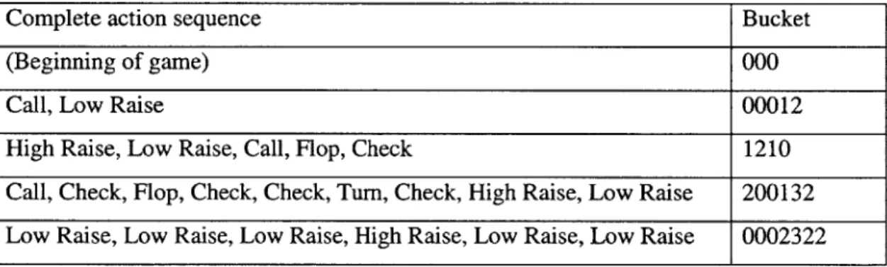
Table 3.1 gives some examples of how full action sequences are mapped to buckets.
Complete action sequence Bucket
(Beginning of game) 000
Call, Low Raise 00012
High Raise, Low Raise, Call, Flop, Check 1210
Call, Check, Flop, Check, Check, Turn, Check, High Raise, Low Raise 200132 Low Raise, Low Raise, Low Raise, High Raise, Low Raise, Low Raise 0002322 Table 3.1 examples of action sequences mapping to buckets. The opponent is the first to act in all of the examples.
Using the abstractions mentioned above, the number of information sets can be reduced to 105_106, a large but much more manageable size. The set of bucketed information sets I is now equivalent to S x H, where S is the set of bucketed action sequences and H is the set of bucketed hand strengths.
3.2 Generalizing across Information Sets
While there is no longer a memory constraint problem in representing the opponent strategy, it would still take an impractically large number of games to obtain enough observations in each information set to accurately estimate the mixed strategy. Even after using abstractions to shrink the number of information sets, it is still far greater than the number of observations of opponent actions in normal game play. Professional human player can get a good sense of their opponent after just a few hundred games, so we know that playing millions of hands should not be necessary.
To deal with this issue, we must generalize about values in information sets that have few or no observations, using the assumption that the values in different information sets are not independent to each other. The space over all possible strategies is in no way uniform. With a large dataset of heads-up hand histories between different players, we can see examples of the type of strategies real players use. Suppose our abstraction of the opponent's strategy is a JIxIAI matrix ir, where I is the set of bucketed information sets and A is the number of bucketed actions (4 in this case), then 7ria is the frequency the opponent chooses action a in information set i. We can estimate these frequencies for each player in the dataset. The goal, however, is to be able to estimate this matrix for a new opponent that the agent is facing even with a low number of observed actions.
3.2.1 Data Mining
We obtained a dataset of 7 million heads-up games between thousands of players on a popular online poker casino called PokerStars. Unfortunately one immediate problem that came up during data mining is that so few of the games revealed the players' hole cards, preventing us from finding out the hand strength of the players. This is due to the nature of the game itself, because players often fold before reaching the showdown if they believe their hand is beaten, and hole cards are not shown if a showdown is not reached. To deal with this issue, we decided to first ignore hand strengths for the moment and only produce a mapping from action sequence to probability distribution over actions using the dataset. Then a heuristic is used to reconstruct a full scale strategy matrix 7r that includes the hand strength.
3.2.2 Strategy Reconstruction
Our goal is to construct a function f1 that take as input any probability distribution over actions observed without regard to hand strength, d E D, where D is the set of all such distributions, and output functions
f2:
H -+ D which maps hand strengths h E H to different distributions. d is a vector <f, c, rl, r2>, where f is the probability of folding, c is the probability of calling, rl the probability of raising below or equal to pot, and r2 the probability of raising above pot. For simplicity in notations later, we will say that the 4 actions have risks of 0, 1, 2, and 3 associated with them respectively.In order to construct function f 1, we need to make a number of assumptions based on rational play.
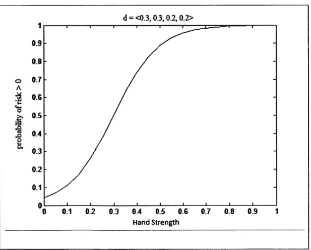
1. The higher the risk associated with the action the opponent takes, the stronger his hand strength is likely to be.
2. The probability of taking an action that has at least some risk value v is modeled by a logistic curve with respect to hand strength as shown by an example in Figure 3.1. d =<0.3, 0.30.2,0.2>
0.9-
0.8-o 0.7-A0.6-0.5
OA --0 0.3- 0.2-0.1 0 0.1 0.2 0.3 0.4 0.5 0.6 0.7 0.8 0.9 Hand StrengthFigure 3.1 shows an example of the probability of not folding with respect to hand strength when d = <0.3, 0.3, 0.2, 0.2>.
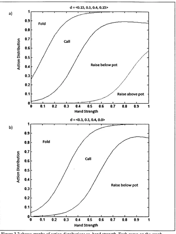
The first assumption is rather obvious. The stronger the hand is, the more likely the player will win at show down. Therefore, it is beneficial to bet more when the chance of winning is higher. For the second assumption, a number of other curves such as a step function or linear function could have been chosen. If we used a step function, the opponent model would end up being a pure strategy which is not realistic. A linear function could be reasonable, but we ultimately chose the logistic function in order to have a tipping point at which the probability of taking a certain amount of risk drops off quickly. Like the graph in Figure 3.1, the probability of taking risk of at least 2 and the probability of taking risk of 3 have similar shapes. Each of the curves is parameterized by c + ri + r2, ri + r2, or r2, respectively. These values shift the curves either to the left or right. Figure 3.2 and 3.3 shows graphs of hand strength to action probabilities that were computed with our algorithm with distributions d =< 0.15, 0.3,0.4,0.15 > and d =<
d = <0.15,0.3,0.4,0.15> 0 0.1 0.2 0.3 0.4 0.5 0.6 0.1 0.8 0.9 1 Hand Strength d =<0.3,0.3,0.4 ,0.0> 0 0.1 0.2 0.3 0.4 0.5 0.6 0.7 0.8 0.9 Hand Strength
Figure 3.2 shows graphs of action distributions vs. hand strength. Each curve on the graph represents probability of risk > c, for c = 0, 1, 2, 3. Between the curves are the probabilities of
a) I C 0 0.9 0.8 037 0.6 0.5 0.4 0.3 0.2 0.1 Fold Call
Raise below pot
-'Raise above pot
0 1 b) C 0 .0 ti 0. 0. 0. 0. 0. 0. 0. 0. 0- 9-8 Fold 7 - 6-'5
4-Raise below pot
3
.2
1 0.9 0.8 0.7 O.6 0.5 0.4 0.3 0.2 0.1 0 0.1 0.2 0.3 0.4 0.5 0.6 0.7 08 0.9 1 Hand Strength d =<0.3,0.3,0.4,0.0>
~1.
FoldRaise below pot
call
0.1 0.2 0.3 0.4 0.5 0.6 0.7
Hand Strength
0.8 0.9 1
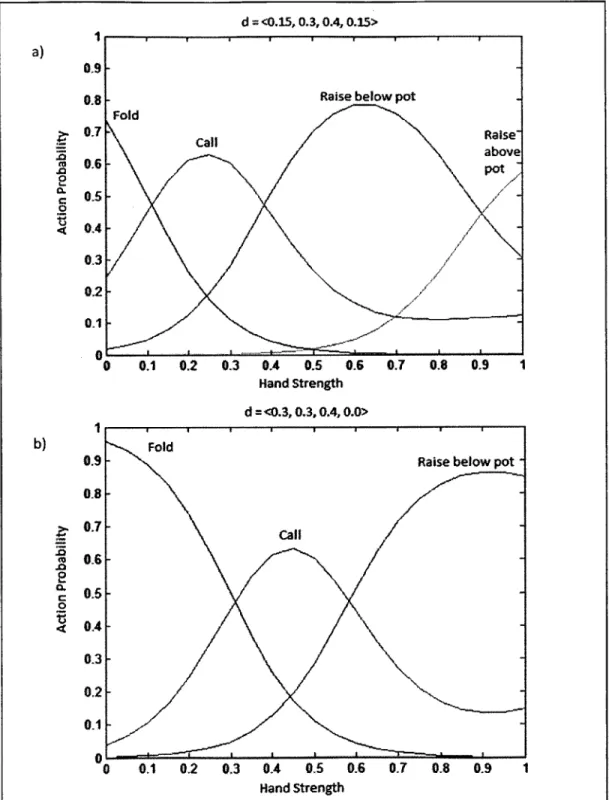
Figure 3.3 shows action probabilities vs. hand strength individually. The value of the curves in the graphs here are essentially the difference between the curves in Figure 3.2.
Raise below pot Fold Call Raise" above pot -- / a) 0 0 b) 0.9 OR . 0 0.8 0.7 0.6 0.6 0.4 0.3 0.2 0.1
0
0 d = <0.15, 0.3,0.4, 0.15> I A ...A-Using this method, the full strategy can be reconstructed for the players in the dataset. However, understandably this reconstructed strategy is not as accurate as if we had built it with the knowledge of all the hole cards, and we hope to change this once more data is obtained in the future.
3.2.3 Estimating Strategy of New Opponents
Now that we have a dataset of full strategies for thousands of real players, we can use it to help estimate the strategy of a new opponent. The distribution of strategies that players take on is most likely a smooth function, meaning if frequencies in a subset of the
strategy matrix between two players are very similar, then it is more likely for the rest of the strategy matrix to have similar frequencies between them as well. Using this idea, we can estimate the frequency of actions in information sets with few or no observations for a new opponent by taking a weighted average over strategies in the dataset that are similar to the new opponent's in the observed information sets.
To calculate the weight, we came up with a distance metric between observations from the new opponent to strategies in the dataset. To calculate this distance, first a raw
opponent strategy is computed using frequency of observations in each information set. If the information set has no observation, the action distribution defaults to uniform. The action distribution each information set maps to is treated as a vector, and we find the Euclidian distance between distributions in each information set between the raw
two strategies is the average of these Euclidian distances weighted by the number of observations in each information set.
The weight of each strategy in the dataset then became the inverse square distance between itself and the new opponent. The strategy of the new opponent is then shifted toward the weighted average of the dataset. The amount of shift depends on the number
of observations in each information set; the more observation, the less the shift. For example the frequency of actions in information sets with zero observations is completely replaced by the weighted average, and ones with over 100 observations are not shifted at all.
Chapter 4
Decision Making
Using the opponent model to compute an appropriate action is the second component of the poker agent. First, the poker agent will track the uncertainty in the opponent's hole cards with Bayesian inference. Then, it will estimate an expected return for each
available action choice. Finally, it will calculate a mixed strategy based on the expected returns.
4.1
Opponent Hole Card Distribution
To clearly define the uncertainty in the opponent's hole cards, the agent will store a probability distribution over every possible hole card combination. This distribution is essentially the belief state, and it is initialized to uniform at the beginning of each hand. For each action that the opponent makes, we will update the distribution as shown in Figure 4.1.
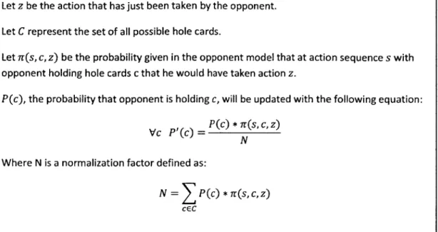
Let z be the action that has just been taken by the opponent. Let C represent the set of all possible hole cards.
Let 7r(s, c, z) be the probability given in the opponent model that at action sequence s with
opponent holding hole cards c that he would have taken action z.
P(c), the probability that opponent is holding c, will be updated with the following equation:
VC P'(c) = P(c) * 7r(s, c, z)
N
Where N is a normalization factor defined as:
N = P(c) * r(s, c, z) CEC
Figure 4.1 shows how the agent updates the probability distribution of opponent's hole cards.
4.2 Estimating Expected Return
To estimate the expected return of different actions, we will use a method similar to David Silver's Monte-Carlo planning for large POMDPs [13]. For each available action an expectation will be calculated by averaging over a number of simulations that plays out the rest of the hand. In each simulation the opponent will be assigned a pair of hole cards based on the distribution mentioned in the previous section. Future community cards will be generated uniformly at random, and opponent's actions will be generated based on the opponent model. The main difference between the method we implemented and the original by David Silver is that instead of also computing the expectations of different actions in child nodes, we only care about the actions from the current decision node. This means a lower number of simulations will need to be run to arrive at a
reasonably accurate expectation. The question now is what rollout policy to use when picking subsequent actions for the agent itself in the simulation.
4.2.1 Uniformly Random Action Selection
A naive method of similarly calculating the expectation for actions in later nodes and picking the best one would not be possible because the number of nodes in the tree, and therefore computational cost, is too high. A feasible option would be to randomly select later actions for the agent even though this does not accurately reflect how the agent really will play in the future.
4.2.2 Self-Model Action Selection
An alternative method is to let the agent keep a strategy model of itself exactly the same way it keeps track of the opponent model. It can then use the self-model to generate actions during simulation at the same speed as generating opponent actions. We compared the two methods against bench mark computer agents in Section 5.2.
The agent always chooses 1 of 4 possible actions. It can fold, check/call, raise 0.7 times the pot, or raise 1.5 times the pot. Fold always has an expected return of exactly 0,
so no simulation is necessary. The other three actions go through 100 simulations each. At the end of each simulation the reward is calculated by taking the pot won (if any) and
subtracting the total amount of chips committed since the beginning of simulation. Any chips that were committed in the action sequence before simulation started are considered
sunk cost and are not subtracted from the reward. The expected reward of the action will simply be the average over the rewards from each simulation.
4.3
Calculating Strategy using Expected Returns
Once simulations are over, we get a 4-tuple of expected returns for the 4 action. If the agent simply chose the action with the highest return, it would be playing the best-response pure strategy which also makes itself exploitable. Since we want a robust counterstrategy, the agent needs to come up with a mixed strategy based on the returns. We came up with the following rules to calculating a mixed strategy.
1. Any action that has negative expected returns will have zero probability. 2. The ratio of at which actions with positive expected returns will be chosen is
equal to the ratio of their returns.
3. If no action has positive expected return, then the agent will always fold. With these rules, the best action will always have the highest probability of being chosen. However it still allows the agent to other actions at times to be less predictable. Rule number 2 uses that particular ratio because it is somewhat reasonable, but different ratios may be tested in the future. One may notice that there are still instances where the agent will still play a single action 100% of the times. This fact does not necessarily make the agent more exploitable because there are legitimate times when there should only be one choice. For example, if the opponent bets all his chips while the agent is holding cards that are impossible to win, then the only good option is to fold.
Chapter
5
Results
5.1 Duplicate Poker
Poker is a game of high variance. In order to conclude with statistical significance that one poker player is better than another, we would normally need to see a very large
number of hands played. To compare computer poker agents, we could greatly reduce the variance by playing duplicate poker.
In duplicate poker, two players will simultaneously play against each other at two different tables. The exact same hole cards and community cards will be dealt at both table, but the position of the players will be reversed on one of the tables. In practice of course, the two matches can occur one after the other as long as memories of the previous match are erased when the duplicate match starts.
Duplicate poker is widely used in computer poker research, because it reduces the number of hands needed, and therefore time cost, when evaluating poker agents.
5.2
Experiments
The two agents whose performance we are interested in are:
1. MC-Random: Agent picks actions for itself uniformly at random during simulation. 2. MC-Self-Model: Agent keeps track of a strategy model of itself and uses it to
generate actions during simulation.
To test the computer agent, we created a number of benchmark agents to play against. The benchmark agents are the following:
1. No-Model: Agent uses a default model of the opponent (model when there are no observations) and never updates it.
2. RaiseBot: Agent will always raise 0.7 times the pot.
3. CallBot: Agent will always call, or check when appropriate.
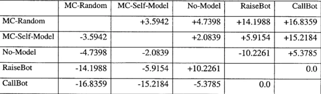
For the experiment, we ran 10000 hands of duplicate poker between every pair of the above agents. Each agent starts with 100 big blinds at the beginning of each hand. The results are in Table 5.1.
MC-Random MC-Self-Model No-Model RaiseBot CallBot
MC-Random +3.5942 +4.7398 +14.1988 +16.8359
MC-Self-Model -3.5942 +2.0839 +5.9154 +15.2184
No-Model -4.7398 -2.0839 -10.2261 +5.3785
RaiseBot -14.1988 -5.9154 +10.2261 0.0
CallBot -16.8359 -15.2184 -5.3785 0.0
Table 5.1 shows the results from matches played between pairs of computer agents. Values in the table are average number of big blinds won per hand by agents to the left of the row.
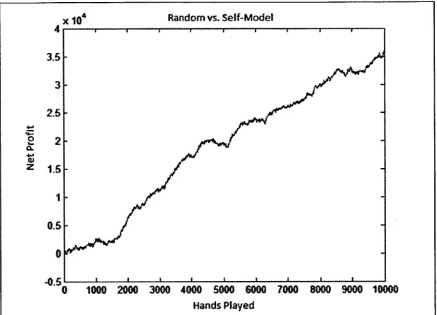
Contrary to our expectations, MC-Random performed better than MC-Self-Model. In fact, it won more chips in each of the benchmark matches and came out positive in the match between the two. Figure 5.1 shows the amount MC-Random won from MC-Self-Model over the course of the 10000 hands.
0 z Random vs. Self-Model <O 4 4 3.5 3 2.5 2 1.5 1 0.5 0 -05 C 1000 2000 3000 4000 5000 6000 7000 8000 9000 10000 Hands Played
Figure 5.1 graphs the net profit of MC-Random as the match against MC-Self-Model progressed.
In 10000 hands of duplicate poker against MC-Self-Model, MC-Random made a total profit of 35942 big blinds with a standard deviation of about 4813, meaning we can conclude without a doubt that MC-Random is indeed superior. However, what is the reasoning behind this result? Why would randomly picking actions during simulation
have significant advantage over the seemingly more rational approach using a self-model? One possible answer is that because both agents are adapting to each other's strategies, the self-model may not be changing fast enough to reflect the agent's true current strategy. Using the outdated self-model during simulation somehow ended up biasing against itself, giving the agent with the simpler approach an advantage.
There are several other results in Table 5.1 that are worth mentioning. Both agents MC-Random and MC-Self-Model performed better than No-Model against the other benchmarks, meaning that the opponent modeling proves to be useful in this case. The agent No-Model did very poorly against the bot that always raised. Other than not updating the opponent model, the rest of No-Model is exactly the same as MC-Random. The reason it lost against RaiseBot is that it folded way too often thinking that RaiseBot has very strong hands. Because it never keeps track of how often the opponent is raising, it updates its belief state as if playing against a normal opponent, placing too much weight on strong opponent hole cards.
Finally, we see that RaiseBot did better than CallBot in all of their respective matches. While both agents are just about as simple as possible, this supports the notion among poker players that being aggressive is better than being passive.
5.3
MIT Poker Competition
The second annual MIT Poker Competition was held in January of 2012. About 27 teams submitted computer agents to play in matches of three-player poker. Our agent, Chezebot,
which is based on most of the concepts described in this thesis but with a number of modifications to fit the three-player format, placed first in the competition. The only
major conceptual difference was in the decision making component. Due to time constraints that did not make simulations possible, the agent evaluated its hand strength against the belief state of the opponent's hole cards and used a heuristic to convert the hand strength into a mixed strategy.
Chapter 6
Conclusion and Future Work
6.1 Conclusion
In this thesis, we have presented an opponent modeling approach to creating a computer poker agent. First we discussed the challenges in modeling a strategy for the game of poker and presented corresponding solutions. We also described the method used to estimate the strategy of new opponents with the help of data mining.
Next we showed how the computer agent makes use of the opponent model to arrive at a robust counterstrategy against that opponent. In the process, we described the belief state update in the agent as response to observations, and we discussed a number of simulation techniques used to estimate expected return of different actions.
Finally, experimental results are presented in which duplicate poker matches are used to evaluate the performance of different versions of the agent against benchmarks.
6.2 Future Work
Our agent now plays only at a low to medium amateur level. A number of future changes could be made to improve its performance.
6.2.1 Improving data mining
Due to the lack of hole card information in our dataset, currently a heuristic is needed to convert the mapping from action sequence to action distribution into a full scale strategy. This greatly decreases the accuracy of the list of strategies from players in the dataset. If we are able to use a large dataset of hand histories that includes hole cards, then it would remove the need for a heuristic and allow us to calculate a much better opponent model from the dataset.
6.2.2 Choosing Action Based on Opponent's Exploitability
Against an opponent that plays a static strategy, using the best-response would be the optimal strategy. However, if the opponent is a good player who also adapts quickly, then it would be wiser to play closer to a Nash-Equilibrium. Therefore, we can try to
approximate how well the opponent adapts to determine what strategy our agent will use, moving toward equilibrium when results seem unfavorable [4].
Between each hand (or a number of hands), the agent can measure how well its own strategy is exploiting the opponent by measuring the change in profit per hand.
Figure 6.1 illustrates a visual representation of the balanced strategy and shows how it is calculated.
Exploitability should be directly proportional to profit per hand. If profit rate is high or increasing, then it would show that the opponent is not adapting quickly enough, and the
agent can play slightly closer to the best response. If the profit rate is low or decreasing, then the agent will play a more mixed strategy. An exploit factor between 0 and 1 is
stored to indicate the balance between equilibrium and best response as shown in Figure 6.1. This factor increases or decreases based on the change in exploitability. This idea is not new as it was also mentioned in (Bowling, M., et al. 2007) as a possible
implementation of a robust counter-strategy, but it may still be an improvement from using the same counter-strategy without considering profitability [1].
e = Exploitability Factor A = Equilibrium B = Best Response C = (1- e) * A + e * B Strategy Space A C B
Bibliography
[1] Bowling, M., Johanson, M. and Zinkevich, M., "Computing Robust Counter-Strategies", University of Alberta, 2007.
[2] FIDE Top Players. 2012. World Chess Federation. 26 Aug. 2012. <http://ratings.fide.com/top.phtml?list=men>.
[3] Gilpin, A., Sandholm, T., "Better Automated Abstraction Techniques for Imperfect Information Games, with Application to Texas Hold'em Poker", Carnegie Mellon University, 2007.
[4] Groot, Bastiaan de., "Wolf-Gradient, a multi-agent learning algorithm for normal form games", Master's thesis, University of Amsterdam, 2008.
[5] Johanson, M.B., "Robust strategies and counterstrategies: Building a champion level computer poker player", Master's thesis, University of Alberta, 2007.
[6] Jonathan, R., Watson, I., "Computer poker: A review", Artificial Intelligence, 2011. [7] Kan, M. H., "Postgame analysis of poker decisions", Master's thesis, University of
Alberta, 2007.
[8] Oliehoek, F., "Game theory and AI: a unified approach to poker games", Master's thesis, University of Amsterdam, 2005.
[9] Sandholm, T., "The State of Solving Large Incomplete-Information Games, and Application to Poker", Carnegie Mellon University, 2011.
[10] Schaeffer, J., et al., "Checkers Is Solved," Science Vol. 317, 2007.
[11] Schauenberg, T., "Opponent modeling and search in poker", Master's thesis, University of Alberta, 2006.
[12] Schnizlein, D., Bowling, M. and Szafron, D., "Probabilistic state translation in extensive games with large action sets", UCAI, 2009.
[13] Silver, D., Veness, J., "Monte-Carlo Planning in Large POMDPs".
[14] The SSDF Rating List. 2012. Swedish Computer Chess Association. 26 Aug. 2012. <http://ssdf.bosjo.net/list.htm>.
[15] Zinkevich, M., Johanson, M., Bowling, M., and Piccione, C., "Regret minimization in games with incomplete information", University of Alberta, 2007.