The economic impacts of climate change : evidence from agricultural profits and random fluctuations in weather

II I

III

1 1 II II I 1 1

3

9080

02617 9306

_W: , iwiiiM\'-wx\\y,

HB31

.M415

no.

04-26

2006b

li

If"

Digitized

by

the

Internet

Archive

in

2011

with

funding

from

Boston

Library

Consortium

Member

Libraries

,

UfcWt

HB31

.M415

Ac.04-Massachusetts

Institute

of

Technology

Department

of

Economics

Working

Paper

Series

The

Economic

Impacts

of

Climate

Change:

Evidence

from

Agricultural

Profits

and

Random

Fluctuations

in

Weather

Olivier

Deschenes

Michael

Greenstone

Working

Paper

04-26

July

2004

Revised:

January

2006

Revised:

August

2006

Room

E52-251

50

Memorial

Drive

Cambridge,

MA

02142

This

paper

can

be

downloaded

without

charge from

the Social

Science

Research

Network

Paper

Collection at

MASSACHUSETTS

INSTITUTE

OF

TECHNOLOGY

The

Economic

Impacts

of

Climate

Change:

Evidence

from

Agricultural

Profits

and

Random

Fluctuations

in

Weather*

Olivier

Deschenes

University

of

California,

Santa

Barbara

Michael

Greenstone

MIT

and

NBER

Previous

Version:

January

2006

This

Version:

August

2006

We

thank

the late

David

Bradford

for initiating a

conversation

that

motivated

this paper.

Our

admiration

for

David's

brilliance as

an economist

was

only

exceeded

by

our

admiration

for

him

as a

human

being.

We

are grateful for the especially valuable criticisms

from

David Card and

two

anonymous

referees.

Orley

Ashenfelter,

Doug

Bernheim,

Hoyt

Bleakley,

Tim

Conley,

Tony

Fisher,

Victor

Fuchs,

Larry

Goulder,

Michael

Hanemann,

Barrett

Kirwan,

Charlie Kolstad,

Enrico

Moretti,

Marc

Nerlove,

Jesse Rothstein,

and

Wolfram

Schlenker provided

insightful

comments.

We

are also grateful for

comments

from

seminar

participants atCornell,

Maryland,

Princeton, University

of

Illinois at

Urbana-Champaign,

Stanford, Yale, the

NBER

Environmental

Economics

Summer

Institute,

and

the

"Conference

on

Spatial

and

Social Interactions in

Economics"

at the University

of

California-Santa Barbara.

Anand

Dash,

Elizabeth

Greenwood,

Ben

Hansen,

Barrett

Kirwan,

Nick

Nagle,

and

William

Young

provided

outstanding research

assistance.

We

are

indebted

to

Shawn

Bucholtz

at the

United

States

Department

of

Agriculture

for

generously

generating

weather

data for this analysis

from

the

Parameter-elevation

Regressions

on

Independent Slopes

Model.

Finally,

we

acknowledge

The

Vegetation/Ecosystem

Modeling and

Analysis

Project

and

the

Atmosphere

Section,

National

Center

for

Atmospheric

Research

foraccess to the Transient

Climate

database,

which

we

used

to obtain regional climate

change

predictions.

Greenstone

acknowledges

generous

funding

from

the

American

Bar

Foundation,

the

Center

for

Energy and

Environmental

Policy

Research

at

MIT,

and

the

Center

for

Labor

Economics

at

Berkeley

for hospitality

and

support

while

working on

this paper.

Deschenes

thanks

the

UCSB

Academic

Senate

for financial

support

and

the Industrial Relations Section atPrinceton University for their hospitality

and

support

while

working on

this paper.

The

Economic

Impacts

of

Climate

Change:

Evidence

from

Agricultural

Output and

Random

Fluctuations

in

Weather

ABSTRACT

This paper measures the

economic

impact ofclimate

change

on

US

agricultural land

by

estimating the

effect ofthe

presumably

random

year-to-year variation in temperature and precipitation

on

agricultural

profits.

Using

long-run climate

change

predictions

from

the

Hadley

2

Model,

the preferred estimates indicate that climate change will lead to a $1.3 billion (2002$) or

4.0%

increase in annual profits.

The

95%

confidence interval ranges

from

-$0.5 billion to $3.1 billion

and

the impact is robust to a

wide

variety ofspecification checks, so large negative or positive effects are unlikely. There is considerable heterogeneityinthe effectacross the country withCalifornia'spredictedimpact equalto-$0.75 billion (or

nearly

15%

ofstate agricultural profits). Further, the analysis indicates that the predicted increases in

temperature

and

precipitation will have virtually

no

effect on yields

among

the

most

important crops,

which

suggest that the small effect on profits are not due to short-run price increases.

The

paper also

implements

the hedonic approach that is predominant in the previous literature and finds that it

may

be

unreliable, because it produces estimates ofthe effect ofclimate change that are extremely sensitive to

seemingly

minor

decisions about the appropriate control variables, sample and weighting. Overall, the findings contradict the popular

view

that climate

change

will have substantial negative welfare consequences forthe

US

agricultural sector.

Olivier

Deschenes

Department

of

Economics

2127 North

Hall

University

of

California

Santa

Barbara,

C

A

93

1

06-92

1 email: olivier(5)econ.

ucsb.edu

Michael

Greenstone

MIT,

Department

of

Economics

50

Memorial

Drive,

E52-391B

Cambridge,

MA

02142

and

NBER

Introduction

There is a

growing

consensus that emissions of greenhouse gases due to

human

activity will lead to higher temperatures and increased precipitation. It is thought thatthese changes in climate will impact

economic

well-being. Since temperature and precipitation are direct inputs in agricultural production,

many

believe that the largest effects will be in this sector. Previous research on climate

change

is inconclusive about the sign

and magnitude

of its effect on the value of

US

agricultural land (see, for

example,

Adams

1989;

Mendelsohn

et. al 1994

and

1999; Kelly, Kolstad,

and

Mitchell 2005; Schlenker,

Hanemann,

and

Fisher (henceforth,

SHF)

2005,2006).

Most

priorresearch

employs

either the production function or hedonic approach to estimate the effect of climate change.'

Due

to its experimental design, the production function approach provides

estimates of the effect of weather

on

the yields of specific crops that are

purged

of bias due to determinantsofagricultural outputthat are

beyond

farmers' control(e.g.,soilquality). Itsdisadvantageis

that these estimates do not account forthe full range of

compensatory

responses to changes in weather

made

by

profit

maximizing

farmers. For

example

in response to a change in climate, farmers

may

alter theiruseoffertilizers,

change

their

mix

ofcrops,oreven decide touse theirfarmlandforanotheractivity

(e.g.,ahousing complex). Since farmeradaptations arecompletelyconstrainedin theproduction function

approach,itis likely toproduceestimatesofclimate

change

thatarebiased

downwards.

The

hedonic approach attemptsto

measure

directly the effect ofclimate

on

land values. Its clear advantage isthatifland marketsare operating properly, prices will reflectthepresentdiscounted value of

land rents into the infinite future. In principle, this approach accounts for the full range of farmer

adaptations.

However,

its validity rests on the consistent estimation of the effect of climate on land values. Since at least the classic

Hoch

(1958

and

1962) and

Mundlak

(1961) papers, it has

been

recognized that

unmeasured

characteristics(e.g., soilqualityandthe optionvaluetoconvertto a

new

use) are important determinants ofoutput and land valuesin agricultural settings." Consequently, the hedonic approach

may

confound

climate with other factors

and

the sign and

magnitude

ofthe resulting omitted

variables biasis

unknown.

In light ofthe importance ofthe question, this paper proposes a

new

strategy to estimate the

impact of climate

change

on the agricultural sector.

The

most

well respected climate

change

models

predict that temperatures

and

precipitation will increase in the future. This paper's idea is simple

—

we

exploit the

presumably

random

year-to-year variation intemperature andprecipitationto estimatewhether

1

Throughout "weather" refers to temperature and precipitation at a given time and place. "Climate" or "climate

normals"refers to a location'sweather averaged over longperiodsoftime. 2

Mundlak focused on heterogeneity in the skills offanners, but in Mundlak (2001), hewrites, "Other sources of

agricultural profits are higherorlower inyears thatare

warmer

and

wetter. Specifically,

we

estimatethe impacts of temperature

and

precipitation on agricultural profits

and

then multiply

them by

the predicted

change

in climatetoinferthe

economic

impactofclimate

change

in thissector.

To

conducttheanalysis,

we

compiledthe

most

detailed

and comprehensive

dataavailableto

form

a county-level panelon agricultural profitsandproduction, soilquality, climate

and

weather.

These

data

are used to estimate the effect of weather on agricultural profits

and

yields, conditional

on

county and state

by

year fixed effects. Thus, the weather parameters are identified

from

the county-specific deviations in weather aboutthe county averages afteradjustment forshocks

common

to allcounties in a

state. Put another

way,

the estimates are identified

from

comparisons ofcounties within the

same

state that

had

positive weather shocks with ones that

had

negative weather shocks, after accounting for their averageweatherrealization.

Thisvariation is

presumed

to be orthogonaltounobserved determinants ofagricultural profits, so

itoffersa possible solution to theomitted variables bias

problems

thatplague the hedonic approach.

The

approach's primary limitation is that farmers cannot

implement

the full range ofadaptations in response to a single year's weatherrealization. Consequently, its estimates

may

overstate the

damage

associated

with climate

change

or, putanotherway, be

downward

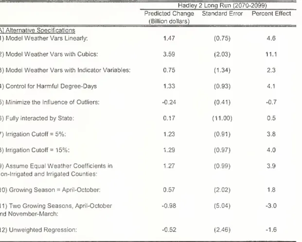
biased.

Figures

1A

and

IB

summarize

the paper's primary findings.

These

figures

show

the fitted

quadratic relationships

between

aggregate agricultural profits,the value ofthe corn harvest,andthe value of the soybean harvest with

growing

season degree-days (1A)

and

total precipitation (IB). (These

measures

of temperature

and

precipitation are the standard in the

agronomy

literature.)

The

key features

oftheseestimates are that they areconditioned

on

county fixedeffects, so the relationships are identified

from

the

presumably

random

variation in weatheracross years within a county.

The

estimating equations

also include state

by

year fixedeffects.

The

vertical linescorrespond tothe national averagesof

growing

season degree-daysandprecipitation.

The

average county ispredictedto

have

increasesof roughly 1,200

degree-days

and

3.0inches duringthe

growing

season

The

striking finding is that all ofthe response surfaces are flat over the ranges ofthe predicted

changes in degree-days

and

inches. If anything, climate change appears to be slightly beneficial for profitsandyields. This qualitativefindingholdsthroughoutthebatteryoftestspresented below.

Using

long-run climate

change

predictions

from

the

Hadley

2

Model,

the preferred estimates indicate that climate

change

will lead to a $1.3 billion (2002$) or

4.0%

increase in annual agricultural

sectorprofits.

The

95%

confidence intervalranges

from

-$0.5 billion to $3.1 billion so large negative or positive effects are unlikely.

The

basic finding of an economically andstatistically small effect is robust

to a

wide

variety of specification checks including adjustment for the rich set of available controls,

and implementing a procedure that

minimizes

the influence of outliers. Additionally, the analysis indicates that the predicted increases in temperature and precipitation will have virtually

no

effect on

yields

among

the

most

important crops (i.e., corn for grain and soybeans).

These

crop yield findings

suggestthatthesmall effectonprofits isnotduetoshort-run price increases.

Although

the overall effect is small, there is considerable heterogeneity across the country.

The

most

striking finding isthat Californiawill be substantially

harmed by

climatechange. Its predicted loss in agricultural profits is

$750

million,

and

this is nearly

15%

of current annual profits in California.

Nebraska

(-$670 million), North Carolina (-$650 million) are also predicted to havebig losses, while the

two

biggestwinners are South

Dakota

($720million) and Georgia ($540million). It is importantto note

thatthese state-level estimatesare

demanding

ofthe dataandtherefore lessprecisethanis ideal.

The

paper also re-examines the hedonic approach that is predominant in the previous literature.

We

find that estimates ofthe effect ofthe

benchmark

doubling of greenhouse gasses on the value of agricultural land range

from

-$200 billion (2002$) to

$320

billion (or

-18%

to

29%), which

is an even wider range than has been noted in the previous literature. This variation in predicted impacts results

from

seemingly

minor

decisionsabout the appropriate control variables, sample,

and

weighting. Despite

itstheoreticalappeal,

we

conclude thatthe hedonic

method

may

beunreliable in this setting.3

The

paper proceeds as follows. Section I provides the conceptual

framework

for our approach.

Section II describes the data sources

and

provides

summary

statistics. Section III presents the

econometric approach and Section

IV

describes the results. Section

V

assesses the

magnitude

of our

estimates ofthe effect ofclimate

change

and

discusses a

number

of important caveats to the analysis.

Section

VI

concludes thepaper.

I.

Conceptual

Framework

A.

A

New

Approach

to ValuingClimate

Change

In this paper

we

propose a

new

strategy to estimate the effects ofclimate change.

We

use a county-levelpaneldatafile constructed

from

the Censuses ofAgricultureto estimatethe effectof weather on agricultural profits, conditional on county and state

by

year fixed effects. Thus, the weather parameters are identified

from

the county-specific deviations in weather about the county averages after adjustment forshocks

common

to all counties in a state. This variation is

presumed

tobe orthogonal to

unobserved determinants ofagricultural profits, so it offers a possible solution to the omitted variables bias

problems

thatappeartoplaguethehedonic approach.

3

Recent research demonstrates thatcross-sectional hedonic equations appear misspecified in a variety ofcontexts

This approach differs

from

the hedonic

one

in a

few key

ways. First, under an additive separability assumption, its estimated parameters are purged of the influence of all

unobserved

time

invariant factors. Second, it is not feasible to use land values as the dependent variable oncethe county

fixed effects are included. This is because land values reflect long run averages of weather, not annual

deviations

from

theseaverages,

and

there isno timevariationinsuchvariables.

Third, although the dependent variable is not land values, our approach can be used to

approximatethe effectofclimate

change on

agricultural land values. Specifically,

we

estimate

how

farm profitsareaffected

by

increases intemperature

and

precipitation.

We

then multiplytheseestimates

by

the predictedchanges inclimateto inferthe impact onprofits. Since thevalue ofland is equal tothe present

discounted stream ofrental rates, it is straightforward to calculate the

change

in land values

when

we

assume

thepredicted

change

inprofits is

permanent and

make

an assumption aboutthediscountrate.

B.

The

Economics of Using Annual

Variation in

Weather

toInfer theImpacts

of

Climate

Change

There are

two economic

issues that could

undermine

the validity of using the relationship

between

short run variation in weather

and

farm profits to infer the effects ofclimate change.

The

first

issue is that shortrunvariation in weather

may

leadto temporary changes in prices thatobscure the true long-run impact of climate change.

To

see this, consider the following simplified expression for the

profits ofarepresentative fannerthat is producing agiven crop andis unable to switch crops in response to shortrun variationin weather:

(1

)

n

=

p(q(w))q(w)

-

c(q(w)),

where

p, q,andc,denoteprices,quantities,

and

costs, respectively. Prices

and

totalcostsare afunction of quantities. Importantly, quantities are a function of weather, w, because precipitation and temperature directly affect yields.

Since climate

change

is a

permanent

phenomenon,

we

would

like to isolatethe longrun

change

in profits. Consider

how

the representativeproducer'sprofitsrespond toa

change

in weather:

(2)

dn

I

dw

=

(dpIdq) (dqI

dw)

_q

+

_(p

-

5c/dq)(Sq/dw).

The

first term is the

change

in prices due to the weather shock (through weather's effect

on

quantities) multiplied

by

the initial level ofquantities.

When

the

change

in weather affects output, the

firstterm is likely to differ inthe short

and

longruns. Consider aweathershock thatreduces output(e.g., (i.e.,

dq

I

dw

<

0). In the short run supply is likely to be inelastic

due

to the lag

between

planting and

harvests, so (dp I _{3q)short Run}

<

0. This increase in prices helps to mitigate the representative farmer's losses

due

tothe lowerproduction.

However,

the supply ofagricultural

goods

is

more

elastic in the long

run as other farmers (or

even

new

fanners) will respond to the price

change

by

increasing output.

Consequently, itis sensible to

assume

that(dp I _<3q)Lon

to-zero.

The

result isthat thefirstterm

may

bepositiveintheshortrun but small, or zerointhelongrun.

The

second term in equation (2) is the difference

between

price and marginal cost multiplied by

the

change

inquantities duetothe

change

inweather. Thistermmeasuresthe

change

inprofits

due

tothe

weather-induced

change

in quantities. It is the longrun effect ofclimate

change

on

agricultural profits

(holding constantcrop choice),andthis isthetermthat

we

would

like to isolate.

Although

our empirical approach relies

on

short run variation in weather, there are several

reasonsthat it

may

bereasonableto

assume

thatourestimates are largely

purged

ofthe influence ofprice

changes (i.e., the first term in equation (2)).

Most

importantly,

we

find that the predicted changes in

climate will

have

a statistically and economically small effecton crop yields(i.e., quantities) ofthe

most

important crops. This finding

undermines

much

ofthe basisforconcerns about shortrun price changes.

Further the preferred econometric

model

includes a full set of state

by

year interactions, so it

non-parametrically adjusts forall factors that are

common

across counties within astate

by

year, such ascrop

price levels.

4

Thus, the estimates will not be influenced

by

changes in state-level agricultural prices. Interestingly,thequalitative results aresimilarwhether

we

control foryearorstate

by

yearfixed effects.5

The

second potential threat to the validity of ourapproach is that fanners cannot undertake the

full range of adaptations in response to a singe year's weather realization. Specifically,

permanent

climate

change

might cause

them

to alter the activities they conduct on their land. For example, they

might switch crops becauseprofits

would

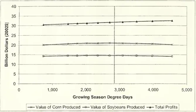
behigherwith analternativecrop.

Figure 2 illustrates this issue. Profitsper acre are

on

the y-axis and temperature is on thex-axis. Forsimplicity,

we

assume

that the influence ofprecipitation andall other

exogenous

determinants (e.g., soil quality)ofprofitsperacrehave been successfully controlled oradjusted for.

The

Crop

1

and

Crop

2 Profit Functions reveal the relationship

between

profits per acre and temperature

when

these crops are chosen. It is evident that crop-specific profits vary with temperatures. Further, the profit-maximizing crop varies with temperature. For example,

Crop

1

maximizes

profits

between

T)

and

Ti,

Crops

1

and

2

produce identical profits at Ti

where

the profit functions cross (i.e., point B), and

Crop

2 is optimal at

temperatures

between

T

2and

T

3.

The

hedonic equilibrium is denoted as the broken line and it represents the equilibrium

4

If production in individual counties affects the overall price level, which would be the case ifa few counties

determine crop prices, or there are segmented local (i.e., geographic units smaller than states) markets for

agricultural outputs,then thisidentificationstrategywill notholdprices constant. Production ofthemostimportant

crops isnotconcentratedina small

number

ofcounties,so

we

thinkthisisunlikely. For example,

McLean

County,

Illinois and

Whitman

County,Washington are the largest producersof cornand wheat, respectively, but they only accountfor

0.58%

and 1.39%oftotalproduction ofthese cropsintheUS.

5

We

explored whether itwaspossible to directlycontrolfor local prices. The

USDA

maintainsdatafiles oncrop

prices at the state-level, but unfortunately these data files frequently have missing values and limited geographic

coverage. Moreover,thestatebyyear fixedeffectsprovideamoreflexible

way

tocontrolfor state-levelvariationin price,becausethey controlforallunobservedfactors thatvaryatthestatebyyearlevel.

relationship

between

temperature andprofits. Inthe longrun

when

farmers can freelyswitchcrops, they will choose to operate along the hedonic equilibrium because it reveals the crop choices that

maximize

their profits. It is

formed

by

the regions of each crop's profit function

where

that crop produces the highestprofitsoverallpotential usesofthatland.

Consider a

permanent

increase in temperature

from

T) to

T

₃. If farmers are able to switch

production

from

crop 1 to crop 2, then their profits can be read off the y-axis at point C.

However,

farmersthatare unabletoswitch crops willearn profitsof

C.

Thus, the long-run

change

inprofits is

C

-A,

but in the short run the difference is

C

-

A,

which

is a

downward

biased estimate ofthe long-run effect. Itisnoteworthythat ifthe

new

temperatureis

>

T| and

<

T

2,then the farmer's short-run

and

long-runprofitsareequal becausethe hedonic equilibriumandthecrop 1 profitfunction areidentical.

This paper's empirical strategy relies

on

year-to-year variation in weather

and

thus it is unlikely

that farmers are able to switch crops

upon

a year's weather realization.

The

import forthe subsequent

analysis is that our estimates ofthe impact ofclimate

change

may

be

downward

biased, relative to the preferred long-run effect that allows for all

economic

substitutions. Ifthe degree ofclimate

change

is "small," however, our estimates are equal to the preferred long-run effect.

One

final note is that in response to year-to-year fluctuations, farmers are able to adjust their

mix

ofinputs (e.g., fertilizer

and

irrigatedwaterusage), so thesubsequent estimates are preferableto productionfunction estimates that

do

notallowforanyadaptation.

II.

Data

Sources

and

Summary

Statistics

To

implement

the analysis,

we

collected the

most

detailed

and comprehensive

data available

on

agriculturalproduction, temperature, precipitation, andsoilquality. This section describes these data

and

reports

some

summary

statistics.

A.

Data

Sources

AgriculturalProduction.

The

data

on

agricultural production

come

from

the 1978, 1982, 1987,

1992, 1997,

and

2002 Censuses

of Agriculture.

The

operators of all farms and ranches

from which

$1,000 or

more

ofagricultural products are

produced and

sold,ornormally

would

have

been

sold, during

the census year are required to respond to thecensus forms. For confidentialityreasons, counties are the

finestgeographicunitof observation inthesedata.

In

much

of the subsequent regression analysis, county-level agricultural profits per acre of farmland is the dependent variable.

The

numerator is constructed as the difference

between

the market value of agricultural products sold and total production expenses across all farms in a county.

The

2002-dataarethebasisforthe analysis.

The

denominatorincludes acresdevotedtocrops, pasture,

and

grazing.

The

revenues

component

measuresthe grossmarket value before taxes ofall agriculturalproducts sold or

removed

from

the farm, regardless of

who

received thepayment. Importantly, it doesnot include

income

from

participation in federal farm

programs

, labor earnings off thefarm (e.g.,

income from

harvesting a

differentfield),or

nonfarm

sources. Thus,itisa

measure

oftherevenue

produced

withtheland.

Total production expenses are the

measure

of costs. It includes expenditures

by

landowners,

contractors, and partners in the operation ofthe farm business. Importantly, it covers all variable costs

(e.g., seeds, labor,

and

agricultural chemicals/fertilizers). It also includes measures of interest paid on

debts

and

the

amount

spent on repair and maintenance ofbuildings,

motor

vehicles,

and

farm

equipment

used forfarm business. Itschieflimitation is that itdoes not account forthe rental rate ofthe portionof

the capitalstock thatisnotsecured

by

a loan, soitisonly a partial

measure

offarms' costofcapital. Just

aswith therevenue variable,the

measure

of expensesis limitedto thosethatare incurred inthe operation

ofthefarmso,forexample, any expenses associatedwith contract

work

forotherfarms isexcluded.7 This

measure

ofprofits per acre is asubstitute forthe ideal

measure

oftotalrent peracre, soitis

instructiveto

compare

the two. Since separate information on rental land isunavailable in the Censuses,

we

used tabulations

from

the 1

999

Agricultural

Economics

and

Land

Ownership Survey

to estimate the

mean

rent per acre (calculated as the "cash rent for land, buildings,

and

grazing" divided

by

the "acres rented with cash"8) as roughly

$35

(2002S).

The

mean

of agricultural profits per acre in the

Census

sample

is about

$42

(2002$), soagricultural profits per acre appear tooverstate the rental rate modestly. Consequently, it

may

be appropriate to multiply thepaper's estimates oftheimpact ofclimate

change

on profits

by

0.83 (i.e.,theestimatedratioofrent to profits) to obtain awelfare measure.

In our replication of the hedonic approach,

we

utilize the variable

on

the value of land and

buildingsasthedependent variable. Thisvariable isavailablein allsixCensuses.

Finally,

we

usethe

Census

datato

examine

the relationship

between

the

two

most

important crops

(i.e., corn for grain and soybeans) yields and annual weather fluctuations.

Crop

yields are

measured

as

totalbushels of productionper acres planted.

SoilQualityData.

No

study ofagricultural productivity

would

be complete withoutdata on soil

6

An

exception is that it includes receipts from placing commodities in the

Commodity

Credit Corporation loan

program. Thesereceiptsdifferfromother federalpaymentsbecause farmersreceive theminexchangeforproducts.

7

TheCensuses contain separate variables forsubcategoriesof revenue (e.g.,revenuesduetocrops and dairysales),

but expenditures are not reported separately for these different types ofoperations. Consequently,

we

cannot provideseparatemeasures ofprofitsbythese categoriesandinstead focus ontotal agricultureprofits.

8

The

estimate ofacresrentedwith cashincludes someacreswheretherentisa combination of cashanda shareof

the output. Consequently, the measure ofrental rate per acre is an underestimate, because the cash rent variable

does not account forthe valueofpayments in crops. Kirwan (2005) reports that

among

rental land where at least

part ofthe rent is paid in cash, roughly

85%

ofthe rental contracts are all cash with the remainder constituting

quality, and

we

rely on the National Resource Inventory

(NRI)

forour

measures

ofthese variables.

The

NRJ

is a massive survey of soil samples

and

land characteristics

from

roughly 800,000 sites that is

conducted in

Census

years.

We

follow the convention in the literature and use a

number

ofsoil quality variables as controls in the equations for land values, profits, and yields, including

measures

of susceptibility to floods, soil erosion (K-Factor), slope length, sand content, irrigation,

and

permeability.

County-level measures are calculated as weighted averages across sites used for agriculture,

where

the

weight is the

amount

ofland the

sample

represents in the county.

Although

these data provide a rich

portrait ofsoil quality,

we

suspect that they are not comprehensive.

Our

approach is motivated

by

this

possibility of

unmeasured

soil quality

and

otherdeterminantsofproductivity.

Climate

and

Weather

Data.

The

climate data are derived

from

the Parameter-Elevation Regressions on Independent Slopes

Model

(PRISM).

9 This

model

generates estimates of precipitation

and

temperature at 4 x 4 kilometers grid cells for the entire

US.

The

data that are used to derive these estimates are

from

the National Climatic

Data

Center's

Summary

ofthe

Month

Cooperative Files.

The

PRISM

model

isused

by

NASA,

the

Weather

Channel,

and

almostallprofessional weatherservices. It is

regardedasone ofthe

most

reliableinterpolation proceduresforclimaticdataon asmallscale.

This

model

anddata areusedtodevelop

month

by

year

measures

ofprecipitation

and

temperature forthe agriculturalland ineachcounty forthe

1970

-

2000

period. This

was accomplished by

overlaying

a

map

ofland uses on the

PRISM

predictions for each grid cell

and

then

by

taking the simple average

across all agricultural land grid cells.

To

replicate the previous literature's application ofthe hedonic approach,

we

calculated the climate normals as the simple average of each county's annual

monthly

temperature and precipitation estimates

between

1970 and

two

years before the relevant

Census

year. Furthermore,

we

followthe convention inthe literature andinclude the January, April, July,

and

October

mean

asindependent variables intheanalysis

(Mendelsohn

et. al 1994

and

1999;

SHF

2005).

Although

the

monthly

averages

may

be appropriate for a hedonic analysis of property values, there are better

methods

for

modeling

the effect of weather on annual agricultural profits.

Agronomists

have

shown

that plant

growth

depends

on the cumulative exposure to heat and precipitation during the

growing

season.

The

standard

agronomic

approach for

modeling

temperature is to convert daily

temperatures into degree-days,

which

represent heating units

(Hodges

1991; Grierson 2002).

The

effect ofheat accumulation is nonlinear since temperature

must

be

above

a threshold for plants to absorb heat

and

below

a ceilingasplants cannot absorb extraheat

when

temperature istoo high.

These

thresholds or

bases vary across crops, but

we

join

SHF

(2006)

and

follow Ritchie and

NeSmith's

(1991) suggested

characterization forthe entire agricultural sector

and

use a base of 46.4° Fahrenheit (F) and a ceiling of

PRISM

was developed by the Spatial Climate Analysis Service at Oregon State University for the National.

Oceanic andAtmosphericAdministration. Seehttp://www.ocs.orst.edu/prism/docs/przfact.html forfurtherdetails.

89.6°

F

(or 8°and 32° C). Ritchie

and

NeSmith

also discuss the possibility ofatemperaturethreshold at

93.2°

F

(34°C),

above

which

increases intemperature areharmful.

We

explore thispossibility below.

We

use daily-level dataon temperatures to calculate

growing

season degree-days

between

April

1 st

and

September

30lh. This period covers the

growing

season for

most

crops, except winter

wheat

(USDA,

NASS

1997).

The

degree-days variable is calculated so that a day with a

mean

temperature:

below

46.4°

F

contributes degree-days;

between

46.4°

F and

89.6°

F

contributes the

number

of

degrees F

above

46.4 degree-days;

above

89.6°

F

contributes 43.2 degree-days.

The

growing

season degree-day

variableisthen calculated

by

summing

the dailymeasures overthe entire

growing

season.

Unfortunately, the

monthly

PRISM

data cannot beusedto directly developa

measure

of

growing

season degree-days.

To

measure

these degree-day variables,

we

used daily-level data on

mean

daily

temperature

from

the approximately 8,000 operational weather stations located in the U.S. during our

sample

period.

These

data

were

obtained

from

theNational Climatic

Data

Center "Cooperative

Summary

ofthe

Day"

Files.

The

construction ofthe sample used is described with

more

details in the appendix.

Our

use ofdaily datato calculate degree-days is an important

improvement

over previous

work

that has

estimated

growing

season degree-days with

monthly

data and distributional assumptions (Thorn 1966;

SHF

2006). Finally, in the specifications that use the degree-days measures of temperature, the precipitationvariable istotal precipitationin the

growing

season,

which

is

measured

with the

PRISM

data

asthe

sum

ofprecipitationacross the

growing

season

months

inthe relevant year.

Climate

Change

Predictions.

We

relyon

two

setsofpredictionsabout climate

change

todevelop our estimates of its effects on

US

agricultural land.

The

first predictions rely on the climate

change

scenario

from

the l sl

IPCC

report associatedwith adoubling of atmosphericconcentrationsofgreenhouse gases

by

the end ofthe 21s1 century

(IPCC

1990;

NAS

1992). This

model assumes

uniform increases (across

months and

regions ofthe

US

andtheir interaction) of5°

F

intemperature

and

8%

in precipitation

andhasbeen usedextensively in theprevious literature

(Mendelsohn

et al. 1994

and

1999;

SHF

2005).

The

second set of predictions is

from

the

Hadley

Centre's 2nd

Coupled Ocean-Atmosphere

General Circulation

Model, which

we

refer to as

Hadley

2 (T. C. Johns et al. 1997). This

model

of

climate is comprised ofseveral individually

modeled components

—

the atmosphere,the ocean, and sea

ice

—

which

are equilibratedusinga"spinup"process.

The Hadley

2

model

and an emissions scenario are

used to obtain daily state-level predictions for January

1994

through

December

2099.

The

emissions

scenario

assumes

a

1%

per year

compounded

increase in both carbon dioxide and

IS92A

sulphate aerosols,

which

implies an increase in greenhouse gas concentrations to roughly 2.5 times current levels by the

end

ofthe21s'_{century. Thisemissions assumption}

isstandard andtheclimate changepredictionis in themiddle ofthe range ofpredictions.

From

these daily predictions,

we

calculate predicted

growing

further details).

10

We

focus onthe

"medium

term"

and

"long run" effects

on

climate,

which

are defined

as averagesof

growing

seasondegree-days

and

precipitationover

2020-2049 and

2070-2099.

B.

Summary

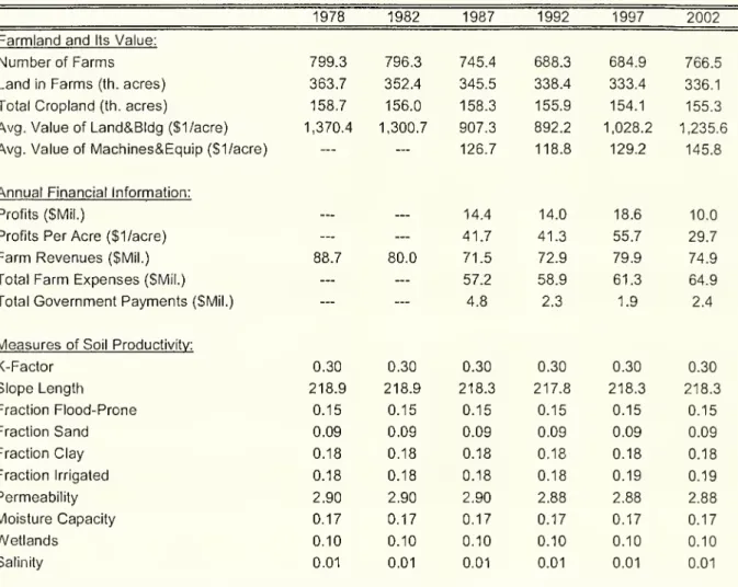
Statistics

Agricultural Finances, Soil,

and

Weather

Statistics. Table 1 reports county-level

summary

statistics

from

the three data sources for 1978, 1982, 1987, 1992, 1997,

and

2002.

The sample

is

comprised

of a balanced panel of 2,268 counties."

Over

the period, the

number

of farms per county

varied

between 680

and 800.

The

total

number

ofacres devotedto farming declined

by

roughly 7.5%.

At

the

same

time, theacreage devotedto cropland

was

roughlyconstantimplying thatthedecline

was

dueto reducedland forlivestock, dairy,

and

poultry farming.

The

mean

average valueofland

and

buildingsper

acre ranged

between

$892 and

SI, 370 (2002$), with the

peak and

trough occurring in 1978

and

1992, respectively.12 (All subsequentfigures arereportedin

2002

constantdollars, unlessnotedotherwise.)

The

second panel details annual financial information about farms.

We

focus

on

1987-2002,

since complete data is only available for these fourcensuses.

During

this period the

mean

county-level

salesofagricultural productsranged

from $72

to

$80

million.

Although

itis not reported here, the share

ofrevenue

from

crop products increased

from

43.7%

to

47.9%

inthis period with the remainder

coming

from

the sale oflivestock

and

poultry.

Farm

productionexpenses

grew from $57

million to

$65

million.

The

mean

countyprofits

from

farmingoperations

were

S14.4million, $14.0million, $18.6million, $10.0

million or $42, $41,

$56 and

$30

per acre in 1987, 1992, 1997,

and

2002

respectively.

These

profit

figures

do

not include

government

payments,

which

are listed atthe

bottom

ofthispanel.

The

subsequent

analysis ofprofits also excludes

government

payments.

The

third panel lists the

means

of the available

measures

of soil quality,

which

are key determinants oflands' productivity in agriculture.

These

variablesare essentially

unchanged

across years since soil

and

land types at a given site are generally time-invariant.

The

small time-series variation in

these variables is due to changes in the composition ofland that is used forfarming. Notably, the only

measure

ofsalinityis

from

1982, so

we

usethis

measure

forall years.

Climate

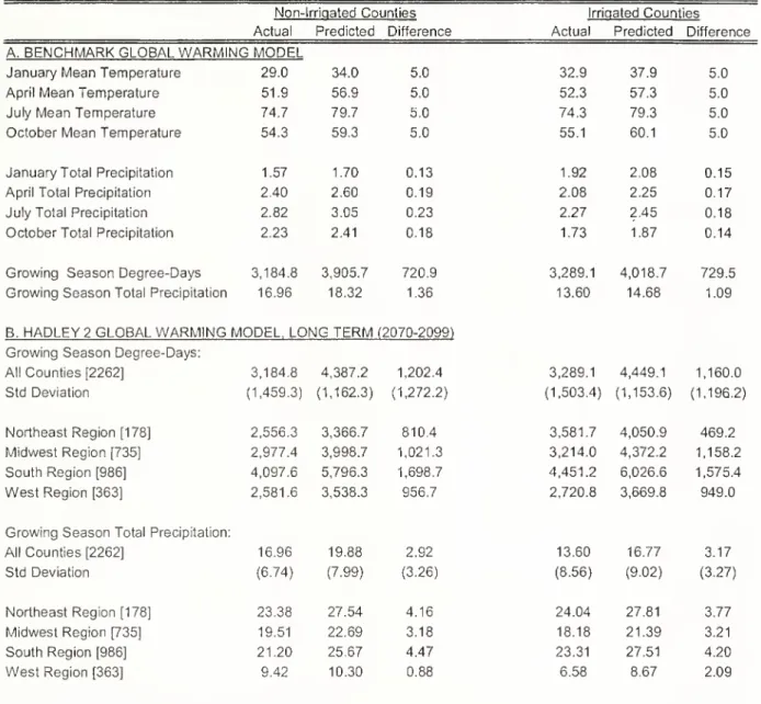
Change

Statistics. Panels

A

and

B

of Table 2 report

on

the predictions of

two

climate

change

models. All entries are calculated as the weighted average across the fixed sample of 2,268

The

Hadley Centre has released a 3rd climate model, which has

some

technical improvements overthe 2nd one.

We

do notuseit for thispaper's predictions, becausedaily predictions are notyetavailable on a subnational scale

overthecourseoftheentire21s'_centuryto

make

_state-level

predictionsaboutclimate.

" Observations from Alaska and Hawaii were excluded.

We

also dropped all observations from counties thathad

missing valuesforoneormoreyearsonany ofthesoilvariables,acres offarmland, acres ofirrigated farmland,per

capita income, population density, and latitude at the county centroid. The sample restrictions were imposed to

provideabalancedpanelofcountiesfrom 1978-2002 forthesubsequentregressions.

All entries are simple averages over the 2,268 counties, except "Average Value ofLand/Bldg (1$ acre)" and,

"ProfitperAcre(l$/acre)",whichareweightedbyacresoffarmland.

counties,

where

the weight is the

number

ofacres offarmland.

The

"Actual"

column shows

the

1970-2000

averages of each ofthe listed variables. There are also

columns

for the predicted values ofthe variables and the difference

between

the actual

and

predicted values. Finally, all ofthe information is

provided separately for non-irrigated

and

irrigated counties.

We

define a county as irrigated if at least

10%

ofitsfarmlandisirrigated, andthisdefinition isused throughoutthe remainder ofthepaper.

Panel

A

reportson the

benchmark

global

wanning

model from

the l sl

IPCC

report,

which

predicts

uniform (acrossseasonandspace) increases of5°

_F

_and

_8%

inprecipitation.

We

mimic

previousresearch

and

focus on January, April, July, and October. There are also entries for

growing

season degree-days

and

totalprecipitation.

Panel

B

reports on the longrun predicted effects

from

the

Hadley

2 Global

Warming

model

for

growing

season degree-days and precipitation. This information is listed forthe country as a

whole and

for each ofthe

Census

Bureau's four regions.

The

model

predicts a

mean

increase in degree-days of roughly 1,200

by

the end of the century (i.e., the

2070-2099

period).

The most

striking regional difference isthe dramatic increase in temperature in the South. Its longrun predicted increase in

degree-days of roughly 1,700

among

non-irrigated counties greatly exceeds the approximate increases of810, 1,000,

and

960

in the Northeast,

Midwest,

and West, respectively.

The

overall average increase in

growing

season precipitation in the long run is approximately 3.0 inches, with the largest predicted increase in the South

and

smallest increase in the West. There is also substantial intra-regional (e.g., at

the state level) variation in the climate

change

predictions, and thisvariation is used in the remainder of

the paperto inferthe

economic

impacts ofclimatechange.

Weather

Variation Statistics. In our preferred approach,

we

aim

to infer the effects ofweather

fluctuations on agricultural profits.

We

focus on regression

models

that include county and year fixed

effects and county and state by year fixed effects. It

would

be ideal ifafter adjustment forthese fixed

effects, the variation in the weather variables that remains is as large as those predicted

by

the climate

change models

usedin thisstudy. In thiscase,ourpredicted

economic

impacts willbeidentified

from

the

data, ratherthan by extrapolationdue tofunctional

form

assumptions.

Panel

C

ofTable 2 reports on the

magnitude

ofthe deviations

between

counties' yearly weather realizations

and

theirlongrun averages after taking out year(row 1) and state-by-year fixed effects(row

2). Therefore, it provides an opportunity to assess the

magnitude

ofthe variation in

growing

season degree-days

and

precipitation after adjustment for

permanent

county factors (e.g.,

whether

the county is usually hot orwet)

and

national time varying factors(e.g.,whether it

was

ahot or

wet

yearnationally) or

state-specific time-varyingfactors (e.g.,whether it

was

ahot or

wet

yearin aparticularstate).

Specifically, the entriesreport the fraction of county

by

yearobservations withdeviations at least as largeas the

one

reported in the

column

heading, averaged overthe years 1987, 1992, 1997,

and

2002.

For example, the

"Removed

State*YearEffects" degree-days

row

indicates that

24.5%,

9.3%,

and

2.2%

of county by year observations haddeviations larger than 400, 800, and 1,200 degree-days, respectively.

The

corresponding

row

for

growing

season precipitation reports that

62.3% 35.3%

and

18.1%

of the

county

by

yearobservations

had

deviations larger than 1.0,2.0,and3.0 inches, respectively.

Temperature

and

precipitation deviations of the magnitudes predicted

by

the climate

change

models

occurinthe data. This is especially true ofprecipitation

where

more

than 1

8%

ofcounty

by

year

observations

have

a deviation larger than 3 inches,

which

roughly equals the predicted increase

from

the

longrun

Hadley

2 scenario.

The

impactofthescenario's

mean

increaseof about 1,200degree-days could be non-parametrically identified, although it

would

come

from

just

2.2%

ofobservations.

However,

5%

of annual county observations have deviations as large as 1,000 degree-days. Finally, it is noteworthy

that differencing out stateweather shocks does not substantially reducethe frequency oflarge deviations, highlightingthatthere areimportantregional patternstoweathershocks.

III.

Econometric

Strategy

A.

The

Hedonic

Approach

This section describes the econometric

framework

that

we

use to assess the consequences of

global climatechange.

We

initiallyconsiderthe hedoniccross sectional

model

thathas been

predominant

in the previous literature

(Mendelsohn

et. al, 1994, 1999;

SHF

2005, 2006). Equation ₍₃₎ provides a

standardformulationofthismodel:

(3) yct

=

X

ct_'P

+

£j 0i f(

W

ic)

+

sct, sct

= a

c

+

uct,

where

yc, isthe value ofagricultural landperacrein countyc inyeart.

The

tsubscript indicates that this

model

could be estimated in

any

year for

which

data is available.

X

ct is a vector of observable

determinants of farmland values,

some

of

which

are time-varying.

The

last term in equation (3) is the stochastic error term, ect, that is comprised of a permanent, county-specific

component,

a

c,

and

an

idiosyncraticshock,ucl.

W

icrepresents aseriesofclimate variables forcountyc.

We

follow

Mendelsohn

etal.(1994) and let iindicate one ofeight climaticvariables. In particular,thereare separate

measures

of temperature

and

total precipitation in January, April, July, and October, so there is one

month

from

each quarter ofthe

year.

The

appropriate functional

form

for each of the climate variables is

unknown,

but in our

replication ofthe hedonic approach

we

follow the convention in the literature

and

model

the climatic

variables with linear and quadratic terms.

As

emphasized by

SHF

(2005), it is important to allow the

effect of climate to differ across non-irrigated and irrigated counties. Accordingly,

we

include interactions ofall theclimate variablesandindicators fornon-irrigated andirrigatedcounties.

The

coefficient vector 9 is the 'true' effect ofclimate on farmland values and its estimatesare usedto calculate the overall effect ofclimate

change

associated with the

benchmark

5-degree Fahrenheit

increase in temperature and eight percent increase in precipitation. Since the total effect

of

climate

change is a linear function of the

components

of the 9 vector, it is straightforward to formulate

and

implement

tests ofthe effects ofalternative climate

change

scenarios

on

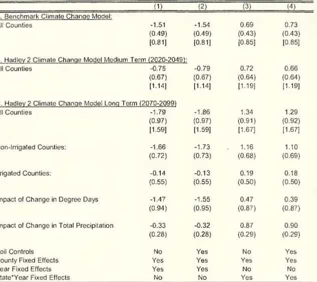
agricultural land values.13

We

will report the standard errors associated with the overall estimate of the effect of climate change.

However,

the total effect of climate change is a function of 32 parameter estimates

when

the climate variablesare

modeled

withaquadratic,soitisnot surprisingthatstatistical significance iselusive.

Consistent estimation ofthe vector 9, and consequently ofthe effect ofclimate change, requires

that

E[f,(W

ic) ec,|

X

ct ]

=

for each climate variable i. This assumption will be invalid if there are

unmeasured permanent

(ac) and/or transitory (ucl ) factors that covary with the climate variables.

To

obtain reliable estimates ofG,

we

collected a

wide

range ofpotential explanatory variables including all

thesoil quality variables listed inTable 1, aswell asper capita

income

and populationdensity. 14

We

also

estimate specificationsthatinclude statefixedeffects.

There are three further issues about equation (3) that bearnoting. First, itis likely that theerror terms are correlated

among

nearby geographical areas. For example, unobserved soil productivity is

spatially correlated, so the standard

OLS

formulas for inference are likely incorrect. In the absence of

knowledge on

the sources

and

the extentofresidual spatial

dependence

in land value data,

we

adjustthe

standard errors for spatial

dependence

of an

unknown

form

following the approach of

Conley

(1999).

The

basic idea is that the spatial

dependence

between

two

observations will decline as the distance

between

the counties increases.15

Throughout

the paper,

we

present standard errors calculated with the

Eicker-

White

formula that allows for heteroskedasticity of an unspecified nature. In addition

we

also

13

Since

we

use a quadratic model for the climate variables, each county's predicted impact is calculated as the

discretedifference in agricultural land values at thecounty's predicted temperatures and precipitationafterclimate

change anditscurrentclimate(i.e.,theaverage overthe 1970-2000period).

14

Previous research suggests that urbanicity, population density, the local price ofirrigation, and air pollution concentrations areimportantdeterminantsofland values (Cline 1996; Plantinga,Lubowski, andStavins2002;

SHF

2005, 2006;

Chay

and Greenstone 2005). Comprehensive data on the price of irrigation and air pollution concentrations are unavailable.

15

More

precisely, theConley(1999) covariancematrix estimatorisobtainedbytakingaweighted average ofspatial

autocovariances. The weights are given by the product ofBartlett kernels in two dimensions (north/south and

east/west), which decline linearly from 1 to 0. The weights reach

when

one ofthe coordinates exceeds a

pre-specified cutoff point. Throughout

we

choose the cutoff points to be 7 degrees of latitude and longitude,

correspondingtodistancesof about500miles.

present the

Conley

standarderrors forourpreferred fixed-effectmodels.

Second, it

may

be appropriate to weight equation (3). Since the dependent variable is

county-level farmland values per acre,

we

think there are

two complementary

reasons to weight

by

the square

root of acres of farmland. First, the estimates of the value of farmland

from

counties with large

agricultural operations will be

more

precise than the estimates

from

counties with small operations,

and

this weight corrects for the heteroskedasticity associated with the differences in precision. Second, the

weighted

mean

ofthedependent variableis equaltothe

mean

valueof farmland peracre inthecountry.

Mendelsohn

et al. (1994, 1999)

and

SHF

(2005) both use the square root ofthe percent ofthe

county in cropland and the square root oftotal revenue

from

crop sales as weights.

We

elected not to

report theresultsbased

on

these approaches in the

main

tables, since the motivation forthese weighting

schemes

is less transparent. For example, it is difficult to justify the assumptions about the

variance-covariance matrixthat

would

motivatetheseweights asasolutiontoheteroskedasticity. Further, although

theseweights

emphasize

the counties that are

most

important to total agricultural production, they

do

so

in an unconventional

manner-B.

A

New

Approach

One

ofthis paper's primary points is that the cross-sectional hedonic equation is likely to be

misspecified.

As

a possible solutionto thisproblem,

we

fit:

(4) yc,

=

a

c

+

y,

+

X

c/p

+

1| 8; fi(Wict)

+

u

ct.

There

are a

number

of important differences

between

equations (4)

and

(3). For starters, the equation

includes afull setof countyfixed effects,

a

c.

The

appealofincluding thecounty fixed effects isthatthey

absorb all

unobserved

county-specific time invariant determinants of the dependent variable.16

The

equationalso includes yearindicators,_yt,that controlforannual differences inthe dependentvariable that

are

common

across counties.

Our

preferred specification replaces theyear fixedeffects withstate

by

year

fixed_{effects (y}st).

The

inclusion ofthe county fixed effects necessitates

two

substantive differences inequation (4),

relative to (3). First, the dependentvariable, _yct, is

now

county-level agricultural profits, instead ofland

values.17 This isbecause land valuescapitalize longruncharacteristicsofsites and, conditional

on

county

fixed effects,annual realizations of weather shouldnot affectlandvalues.

However,

weather does affect farm revenuesand expenditures

and

theirdifferenceis equalto profits.

Second, it is impossible to estimate the effect ofthe long run climate averages in a

model

with

6

Interestingly, the fixed effects model was first developed by

Hoch

(1958 and 1962) and

Mundlak

(1961) to

accountforunobserved heterogeneityinestimatingfarm productionfunctions.

17

Kellyetal. (2005)estimate the cross-sectional relationshipbetween agricultural profitsandclimate.

county fixed-effects,becausethere is

no

temporalvariationin

W

jc

. Consequently,

we

replace the climate

variables with annual realizations of weather,

W,

ct.

We

follow the standard

agronomic

approach and

model

temperature

by

using

growing

season degree-days, defined with abase of 46.4°

F

and

aceiling of

89.6° F. Similarly,

we

model

the effect ofprecipitationon agricultural profitsper acre

by

using

growing

season precipitation.

Once

again,

we

let the effects ofthese variables differ across irrigated and non-irrigated counties. Further,

we

model

them

withquadratics.

The

validity of any estimateofthe impactofclimate

change

basedon equation(4) rests crucially

on

the assumption that its estimation will produce unbiased estimates of the 6vector. Formally, the consistency of each 0, requires E[f,(Wict)

u

ct|

X

ct,

a

c, yst]= 0.

By

conditioning on the county

and

state by

year fixed effects, the 0,'s are identified

from

county-specific deviations in weather about the county averages aftercontrolling forshocks

common

to all counties in a state. This variation is

presumed

tobe orthogonal to unobserved determinants ofagricultural profits, so it provides a potential solution to the omitted variables bias problems that appear to plague the estimation of equation (3).

A

shortcoming of this approach is thatall the fixed effects are likely to

magnify

the importance ofmisspecification due to

measurement

error,

which

generally attenuates the estimated parameters.

IV.Results

Thissection isdivided into threesubsections.

The

firstprovides

some

suggestive evidence on the validity ofthe hedonic approach and then present results

from

that approach.

The

second subsection presents results

from

the fitting of equation (4) to estimate the impact of climate

change

on the

US

agricultural sector. It also probes the distributional consequences ofclimate

change

across the country.

The

third andfinal subsection estimates theeffect ofclimate

change on

cropyieldsforcorn for grainand soybeans, the

two most

important cropsinthe agricultural sectorinterms ofvalue.

A. Estimates ofthe

Impact

of Climate

Changes

from

the

Hedonic Approach

Does

Climate Varywith Observables?

As

theprevious section highlighted, thehedonicapproach relies on the assumptionthatthe climate variables are orthogonal to the unobserved determinants ofland values.

We

begin by

examining

whether these variables are orthogonal to observable predictors offarm

values.

While

this is not aformal testofthe identifyingassumption, there areat least

two

reasons that it

may

seem

reasonable to

presume

that this approach will producevalid estimates ofthe effects ofclimate

when

the observables are balanced. First, consistent inference will not

depend

on functional

form

assumptions on the relations

between

the observable confounders and farm values. Second, the

unobservables

may

be

more

likely tobe balanced (Altonji,Elder, and

Taber

2000).

Table 3

shows

the association

between

theJulytemperature

and

precipitationnormals (calculated

from

1970-2000) and selected determinants offarm values. Tables with the full set of determinants of

farm

values and the temperature and precipitation normals of other

months

are reported in the online

appendix. Panel

A

(B) reports the

means

of county-level farmland values, soil characteristics,

and

socioeconomic

and

locational attributes

by

quartile ofthe July temperature (precipitation) normal.

The

means

are calculated with data

from

the six

Censuses

but are adjusted foryear effects. For temperature (precipitation), quartile 1 refers to the counties with the coldest temperature (least precipitation).

The

fifth

column

reports F-statistics

from

tests that the

means

are equal across the quartiles. Since there are

sixobservations per county, thetest statisticsallows forcounty-specific

random

effects.

A

value of2.37 (3.34) indicates that the null hypothesis can be rejected at the

5%

(1%)

level. Ifclimate

were randomly

assignedacross counties, there

would

be very

few

significantdifferences.

It is immediately evident that the observable determinants of farmland values are not balanced

across the quartiles of weather normals: All ofthe F-statistics

markedly

reject the null hypothesis of

equality across quartiles. In fact, in our extended analysis reported in the online appendix, the null hypothesis ofequalityofthe

sample

means

oftheexplanatory variables across quartiles canberejected at

the

1%

level in 11 1 ofthe 112 cases considered.

18

In

many

cases the differences in the

means

are large, implying that rejection ofthe null is not

simply due tothe

sample

sizes. For example, the fractionofthe land that is irrigated

and

the population

density (a

measure

ofurbanicity or ofthe likelihood of conversion to residential housing) in the county

are

known

tobe important determinants ofthe agriculturalland values,

and

their

means

vary dramatically across quartiles ofthe climate variables. In fact, the finding that population density is associated with agricultural land values

undermines

the validity ofthe hedonic approach to

leam

about climate

change

because density has

no

direct impact

on

agricultural yields. Overall, the entries suggest that the

conventional cross-sectional hedonic approach

may

be biased

due

to incorrect specification of the functional

form

oftheobserved variables

and

potentiallydueto

unobserved

variables.

Replication of

SHF

(2005)

Hedonic Approach.

With

these results in mind,

we

implement

the hedonic approach outlined in equation (3).

We

begin

by

replicating the analysis of

SHF

(2005) using theirdatabased

on

the 1982

Census

of Agriculture

and

programs,

which

they provided.

We

follow their proposed approach and use a quadratic in each ofthe 8 climate variables.

Although

the point oftheir paper is that pooling irrigated

and

non-irrigated counties can lead to biased estimates of climate

parameters inhedonic models, they onlyreport estimatesbased

on

specifications that constrain theeffect

18

We

also divided the sample into non-irrigated and irrigated counties,where a county is definedas irrigated if at least

10%

ofthe farmland is irrigated and the other counties are labeled non-irrigated.

Among

the non-irrigated

(irrigated)counties, the nullhypothesisofequalityofthesamplemeansoftheexplanatoryvariablesacross quartiles.

canberejectedatthe

1%

levelfor 111 (96)ofthe 112covariates.

ofclimate to be the

same

in both sets ofcounties.

Based

on

this approach, the aggregate impact ofthe

benchmark

scenario increases of 5 degrees Fahrenheit in temperatures and

8%

in precipitation on farmland values is -S543.7 billion (2002S) with cropland weights or $69.1 billion with crop revenue

weights. Exceptfor a

CPI

adjustment, these estimatesare identical tothosein

SHF

(2005).

To

probe therobustness ofthese results,

we

re-estimate the hedonic

models

using

two

alternative

sets ofcovariates.

The

first dropsallcovariates, exceptthe climate variables, whilethe second adds state

fixed effects to the specification used

by

SHF.

The

state fixed effects account for all

unobserved

differences acrossstates (e.g., soil quality and stateagriculturalprograms).

The

simple specificationthat only controls for the climate variables produces an estimate of-$98.5 billion with the cropland weights

and

$437.6billionwith thecrop revenueweights.

The

specificationthatadds state fixedeffects produces

estimatesof -$477.8billion

and

$1,034.0 billion.

The

latterfigure

seems

implausible, sinceitis nearly as

largeastheentirevalueofagriculturallandandbuildingsinthe

US, which

was

$1,115billionin 2002.

As

discussedpreviously, our

view

isthatthese

two

sets of weights have

no

clearjustification. In our opinion, the appropriate approach is to weight

by

acres of farmland. Re-estimation ofthe

SHF,

climate variables only, and

SHF

plus state fixed effects specifications with the reconstructed version of

the

SHF

data fileproduces estimatesof $225.1 billion, -$315.4 billion, and-$0.6 billion. Consequently,

the

SHF

findings appearto also berelated tothe choice ofweights. It

seems

reasonable toconclude that

the application ofthe hedonicapproachto the

SHF

datafailsto producerobust estimates ofthe impact of

climate

change

even with a single year of data. In our view, the fragility or non-robustness of this approachisnot

conveyed

adequately intheir article orin

Mendelsohn

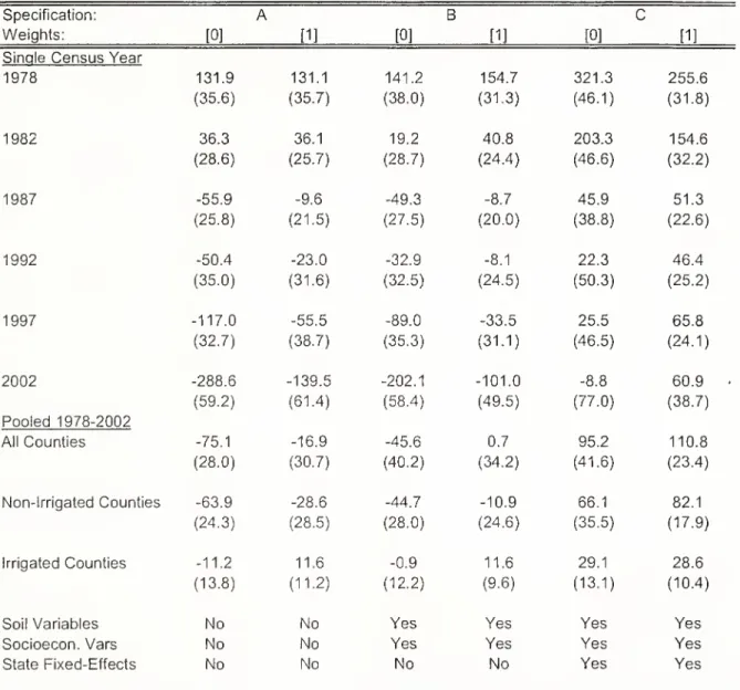
et al.(1994).19

New

Hedonic

Estimates. Table 4 furtherinvestigates the robustness ofthe hedonic approach

by

conducting our

own

broader analysis.

To

this end,

we

assemble our

own

samples

from

the

1978-2002

Censuses

ofAgriculture.

We

maintain the

same

quadratic specificationin each ofthe 8 climatevariables.

There

are

some

important differences

between

our approach

and SHF.

First,

we

fit regressions

that allow the effects ofclimate

on

farmland values to vary in irrigated and non-irrigated counties. In addition, the regressions allow for intercept differences across irrigated and non-irrigated counties but constrain all other parameters to be equal in the

two

sets ofcounties. Second,

we

report standard errors fortheestimatedimpacts. Third,

we

do not truncate the county-specific estimatedimpactsatzero.

The

entries inTable 4 reportthepredicted changes in land values inbillions of

2002

dollars (and their standard errors in parentheses) from the

benchmark

increases of 5 degrees Fahrenheit in

temperatures and

8%

in precipitation.

These

predicted changes are based on the estimated climate

parameters

from

the fitting of equation (3).

The

42

different estimates ofthe national impact on land