A digital spectral analysis technique and its application to radio astronomy.

DOCUMENT ROM, id , -

f

-RESn,:ARCH LA{lRAT':RY OF E,ECTRONICS MA,,ACH ',IU;,r:; i' STI TUTE OF TECHNLOGy

CA.B'd'IRDI G , ,8A':,.SCUSETTS 'U.SA,,

A DIGITAL SPECTRAL ANALYSIS TECHNIQUE AND

ITS APPLICATION TO RADIO ASTRONOMY

SANDER WEINREB

/ a

(

AUGUST 30, 1963

MASSACHUSETTS INSTITUTE OF TECHNOLOGY

RESEARCH LABORATORY OF ELECTRONICS

CAMBRIDGE, MASSACHUSETTS

I

7pL

I _ ___ _ __ _

The Research Laboratory of Electronics is an interdepartmental laboratory in which faculty members and graduate students from numerous academic departments conduct research.

The research reported in this document was made possible in part by support extended the Massachusetts Institute of Tech-nology, Research Laboratory of Electronics, jointly by the U.S. Army (Signal Corps), the U.S. Navy (Office of Naval Research), and the U.S. Air Force (Office of Scientific Research) under Sig-nal Corps Contract DA36-039-sc-78108, Department of the Army Task 3-99-25-001-08; and in part by Signal Corps Grant DA-SIG-36-039-61-G14; additional support was received from the National. Science Foundation (Grant G-13904).

Reproduction in whole or in part is permitted for any purpose of the United States Government.

MASSACHUSETTS INSTITUTE OF TECHNOLOGY RESEARCH LABORATORY OF ELECTRONICS

Technical Report 412 August 30, 1963

A DIGITAL SPECTRAL ANALYSIS TECHNIQUE AND ITS APPLICATION TO RADIO ASTRONOMY

Sander Weinreb

Submitted to the Department of Electrical Engineering, M.I.T., February 1963, in partial fulfillment of the requirements for the degree of Doctor of Philosophy.

(Manuscript received May 23, 1963)

Abstract

An efficient, digital technique for the measurement of the autocorrelation function and power spectrum of Gaussian random signals is described. As is well known, the power spectrum of a signal can be obtained by a Fourier transformation of its autocor-relation function. This report presents an indirect method of computing the autocorre-lation function of a signal having Gaussian statistics which greatly reduces the amount of digital processing that is required.

The signal, x(t), is first "infinitely clipped"; that is, a signal, y(t), where y(t) = 1 when x(t) > 0, and y(t) = -1 when x(t) < 0, is produced. The normalized autocorrelation function, py(T), of the clipped signal is then calculated digitally. Since y(t) can be coded into one-bit samples, the autocorrelation processing (delay, storage, multiplication, and summation) can be easily performed in real time by a special-purpose digital machine - a one-bit correlator. The resulting p y(T) can then be corrected to give the normalized autocorrelation function, px(T), of the original signal. The relation is due to Van Vleck and is px(T) = sin [rpy(T)/2].

A review of the measurement of power spectra through the autocorrelation function method is given. The one-bit technique of computing the autocorrelation function is presented; in particular, the mean and variance of the resulting spectral estimate have been investigated.

These results are then applied to the problem of the measurement of spectral lines in radio astronomy. A complete radio-astronomy system is described. The advantages of this system are: 1) It is a multichannel system; that is, many points are determined on the spectrum during one time interval; and 2) since digital techniques are used, the system is very accurate and highly versatile. This system was built for the purpose of attempting to detect the galactic deuterium line. Results of tests of this system, the attempt to detect the deuterium line, and an attempt to measure Zeeman splitting of the 21-cm hydrogen line are described.

TABLE OF CONTENTS

Glossary vi

I. INTRODUCTION 1

1.1 Statistical Preliminaries 1

1.2 Definition of the Power Spectrum 4

1.3 General Form of Estimates of the Power Spectrum 6

1.4 Comparison of Filter and Autocorrelation Methods

of Spectral Analysis 7

1.5 Choice of the Spectral-Measurement Technique 10

1.6 The One-Bit Autocorrelation Method of Spectral

Analysis 15

II. THE AUTOCORRELATION FUNCTION METHOD OF MEASURING

POWER SPECTRA 17

2.1 Introduction 17

2.2 Mean of the Spectral Estimate 18

a. Relation of P (f) to P(f) 18

b. The Weighting Function, w(nAT) 20

c. Some Useful Properties of P*(f) 23

2.3 Covariances of Many-Bit Estimates of the Autocorrelation

Function and Power Spectrum 23

a. Definitions: Relation of the Spectral Covariance to the

Autocorrelation Covariance 24

b. Results of the Autocorrelation Covariance Calculation 25

c. Results of the Spectral Covariance Calculation 27

2.4 Normalized, Many-Bit Estimates of the Spectrum and

Autocorrelation Function 28

a. Mean and Variance of the Normalized Autocorrelation

Estimate 29

b. Mean and Variance of the Normalized Spectral Estimate 30

III. THE ONE-BIT METHOD OF COMPUTING AUTOCORRELATION

FUNCTIONS 32

3.1 Introduction 32

3.2 The Van Vleck Relation 34

3.3 Mean and Variance of the One-Bit Autocorrelation

Function Estimate 35

3.4 Mean and Variance of the One-Bit Power Spectrum

Estimate 37

CONTENTS

IV. THE RADIO-ASTRONOMY SYSTEM 40

4.1 System Input-Output Equation 40

4.2 Specification of Antenna Temperature 42

a. Correction of the Effect of Receiver Bandpass 42

b. Measurement of T 44

av

c. Measurement of Tr(f+fo ) 44

d. Summary 45

4.3 The Switched Mode of Operation 45

a. Motivation and Description 45

b. Antenna Temperature Equation 48

4.4 System Sensitivity 49

V. SYSTEM COMPONENTS 51

5.1 Radio-Frequency Part of the System 51

a. Front-End Switch and Noise Source 51

b. Balance Requirements 53

c. Shape of the Receiver Bandpass, G(f+fo) 53

d. Frequency Conversion and Filtering 55

5.2 Clippers and Samplers 56

5.3 Digital Correlator 58

VI. SYSTEM TESTS 64

6.1 Summary of Tests 64

6.2 Computer Simulation of the Signal and the Signal-Processing

System 65

a. Definitions and Terminology 65

b. Computer Method 67

c. Results and Conclusions 69

6.3 Measurement of a Known Noise-Power Spectrum 75

a. Procedure 75

b. Results 77

6.4 Measurements of Artificial Deuterium Lines 78

6.5 Analysis of the RMS Deviation of the Deuterium-Line Data 81

a. Theoretical RMS Deviation 81

b. Experimental Results 82

VII. THE DEUTERIUM-LINE EXPERIMENT 85

7.1 Introduction 85

7.2 Physical Theory and Assumptions 86

7.3 Results and Conclusions 90

CONTENTS

VIII. AN ATTEMPT TO MEASURE ZEEMAN SPLITTING OF THE 21-cm HYDROGEN LINE

8.1 Introduction

8.2 Experimental Procedure 8.3 Results and Conclusion

Appendix A

Appendix B

Appendix C

Appendix D

Equivalence of the Filter Method and the Autocorrelation Method of Spectral Analysis

The E1B Method of Autocorrelation Function Measurement

Calculation of the Covariances of Many-Bit Estimates of the Autocorrelation Function and Power Spectrum

Computer Programs

D. 1 Doppler Calculation Program

D.2 Deuterium and Zeeman Data Analysis Program D.3 Computer Simulation Program

Acknowledgment References v 93 93 93 97 98 100 103 106 106 109 113 117 118

GLOSSARY

Symbol Definition

Time Functions

x(t) A stationary, ergodic, random time function having Gaussian statistics.

y(t) The function formed by infinite clipping of x(t). That is, y(t) = 1 when x(t) > 0, and y(t) = -1 when x(t) < 0.

Frequency and Time

Because of their standard usage in both communication theory and radio astronomy, the symbols T and T symbolize different quantities in different sections of this report.

In Sections I-III, T is a time interval and T is the autocorrelation function delay

var-iable. In Sections IV-VIII, T is temperature, and T is either optical depth or

obser-vation time. Some other frequency and time variables are the following: At, k, K, ft

AT, n, N, fs

S

The time function sampling interval is At. A sample of the time function x(t) is x(kAt), where k is an integer. The total number of samples is K. The sampling frequency is ft = 1/At. In most cases At and ft will be chosen equal to

AT and f s, respectively.

The autocorrelation function sampling interval is AT. The samples of the autocorrelation function are R(nAT), where n is an integer going from 0 to N-1. The reciprocal of AT

is f.

The frequency resolution of a spectral measurement (see sec-tion 1.3). It is approximately equal to 1/NAT.

B1 1B2 0 The -db and 20-db bandwidths of a radiometer. The spectrum

is analyzed with resolution Af in the band B1. The sampling

frequencies ft and fs are often chosen equal to 2B2 0.

A known combination of local oscillator frequencies. f

o

Autocorrelation Functions

The true autocorrelation function of x(t).

A statistical estimate of R(T) based upon unquantized or many-bit samples of x(t).

R(T)

GLOSSARY (continued)

Symbol Definition

p(r) or px (T) The true normalized autocorrelation function; P(T) = R(T)/R(O).

t"(T) A statistical estimate of p(¶) based upon unquantized or

many-bit samples of x(t).

p'(T) or pX(T) A statistical estimate of p(T) based upon one-bit samples of y(t). Py(T) The true normalized autocorrelation function of y(t).

p'(T) A statistical estimate of py(T) based upon one-bit samples of y(t).

Power Spectra

The power spectrum is defined in section 1.2.

P(f) The true power spectrum of x(t).

P"(f) A statistical estimate of P(f) based upon unquantized or many-bit samples of x(t).

P (f) The expected value of P"(f).

p(f) The true normalized power spectrum; p(f) = P(f)/R(O).

p"(f) A statistical estimate of p(f) based upon many-bit or unquan-tized samples of x(t).

p'(f) A statistical estimate of p(f) based upon one-bit samples of y(t). p* (f) The expected value of p'(f) and p"(f).

Pc (f) The normalized spectral estimate produced by a one-bit auto-correlation radiometer when its input is connected to a

com-parison noise source.

p' (f) A normalized estimate of the receiver power transfer function, G(f). It is the spectral estimate produced by a one-bit auto-correlation radiometer when the input spectrum and receiver noise spectrum are white.

Sp'(f) The estimate of the difference spectrum that is determined by a switched radiometer; 6p'(f) = p'(f) - p' (f)._c

GLOSSARY (continued)

Symbol Definition

Temperature

Ta(f) The power spectrum available at the antenna terminals

expressed in degrees Kelvin.

Tr(f) The receiver noise-temperature spectrum.

T(f) The total temperature spectrum referred to the receiver input. T(f) = Ta(f) + Tr(f).

Tc(f) The spectrum of the comparison noise source.

Tav The frequency-averaged value of Ttf). The average is weighted with respect to the receiver power-transfer function, G(f).

Ta av The frequency-averaged value of Ta(f).

Tc av The frequency-averaged value of Tc(f) + Tr(f).

Tr av The frequency-averaged value of Tr(f).

ST _av The unbalance temperature; ST _av = T _av - T_{c av}

RMS Deviations

A - with two subscripts will be used to denote an rms deviation of a statistical esti-mate. The first subscript will be a P, R, p or p, and indicates the variable to which the rms deviation pertains. The second subscript will be a 1 or an m, and indicates whether the statistical estimate is based upon one-bit or many-bit samples. Thus, for example, pl is the rms deviation of p'(f), the one-bit estimate of p(f). Statistical esti-1

mates of rms deviations will have a single subscript and a prime or double prime to indicate whether one-bit or many-bit samples are referred to. For example, r' (f) is a statistical estimate of pl(f).

Other Functions

w(T) The function that is used to weight the autocorrelation function

(see section 2.2).

W(f) The spectral scanning or smoothing function. It is the Fourier transform of w(T) (see Fig. 9).

G(f+f ) The receiver power-transfer function. The spectrum at the clipper input, P(f), is equal to G(f+fo ) times the input

temper-ature spectrum, T(f+fo).

GLOSSARY (continued)

Symbol Definition

Special Symbols

x(t) A line over a variable indicates that the statistical average is taken (see Eq. 1).

P (f) An asterisk on a spectrum indicates that it has been smoothed and is repeated about integer multiples of the sampling fre-quency. This operation is discussed in section 2.2.

Tt(f) The one-bit autocorrelation radiometer produces a statistical estimate of an input temperature spectrum such as T(f). The statistical average or expected value of this estimate is equal to Tt(f). The relationship between T(f) and Tt(f) is discussed in section 4.2a. Under proper conditions such as a sufficiently fast sampling rate, Tt(f) is simply a smoothed version of T(f).

I. INTRODUCTION

This report has three main divisions which will be outlined briefly.

1. In Sections I-III, a technique for the measurement of the power spectrum and autocorrelation function of a Gaussian random process is presented. This technique, which will be referred to as "the one-bit autocorrelation method," has the property that it is easily performed digitally; hence the accuracy and flexibility associated with digital instrumentation is achieved. The technique is a multichannel one; that is, many points on the spectrum and autocorrelation function can be determined at one time. A limitation is that the analyzed bandwidth must be less than 10 mc for operation with present-day digital logic elements.

2. The above-mentioned technique is applied, in Sections IV and V, to the problem of the measurement of spectral lines in radio astronomy. In Section IV the composition and theoretical performance of a practical radio astronomy system utilizing the one-bit digital autocorrelation technique is presented. The design of components of this system is discussed in Section V.

3. The system was constructed and extensive experimental results are given in Sections VI-VIII. These results are from laboratory tests of the system, an attempt to detect the galactic deuterium line, and an attempt to measure Zeeman splitting of the 21-cm hydrogen line.

The reader who is interested in the radio astronomy aspects of this report may wish to skip Sections II and III; the results are summarized in radio astronomy terms in Sec-tion IV.

We shall now give some background material, a comparison of filter and autocorre-lation methods of spectral measurement, a classification of spectral measurement prob-lems, and finally, a brief description of the one-bit autocorrelation method.

1.1 STATISTICAL PRELIMINARIES

A brief presentation of some of the statistical techniques and terminology used in this report will now be given. Some assumptions will be stated regarding the statis-tical nature of the signals of interest. For an introduction to statisstatis-tical communication theory techniques, the reader is referred to Davenport and Root, or Bendat.2

The type of signal that is of interest here is the random time function; that is, a signal whose sources are so numerous, complicated, and unknown that exact prediction or description of the time function is impossible. Our interest is in the study of aver-ages of functions of the signal, in particular, the power spectrum, which is defined in

section 1.2.

A random variable, x, is the outcome of an experiment that (at least theoretically) can be repeated many times and has a result that cannot be exactly predicted. The flipping of a coin or the measurement of a noise signal at a given time are two such experiments. The outcome of a particular experiment is called a sample of the random

variable; it is implied that there is a large number of samples (although many samples may have the same value).

The random variable is described by a probability density function, p(x). The statistical average (this will sometimes be called the "mean") of a random variable is denoted by a bar over the quantity that is being averaged such as x. In terms of the probability density function, the statistical average of x is given by

X= x p(x) dx. (1)

-oO

In most signal-analysis cases the random variable is a function of a parameter, such as frequency or time. Thus, there is an infinite number of random variables, one for each value of the parameter. For each random variable there is a large number of samples. This two-dimensional array of sample functions is called a random process.

The concept of a random process with time as the parameter is shown in Fig. 1. For each value of time a random variable, xt , is defined. Each random

var-O (1) (2)

iable has an infinite number of samples, xt , t ... , t The random proc-ess can also be described as having an infinite number of sample functions, x(l)(t), x(2)(t), ... , x(o)(t). (The superscripts will be dropped when they are not needed for clarity.)

Statistical averages, such as xt , are taken vertically through the random-process

o

array, and may or may not be a function of time. Time averages such as I T x(t) dt x()(t) x(2)(t) , , '~~~~~~~~~~~~~~~~ x ()) (t) I I t 0

Fig. 1. A random process.

are taken across the array, and may or may not depend on the sample function chosen. It will be assumed that signals whose power spectra we wish to measure are

2

stationary and ergodic. By this it is meant that statistical averages such as xt, xt ,

o o

and xt xt +T are independent of the time, to, and are equal to the infinite time aver-O o

ages, which, in turn, are independent of the particular sample function. That is,

1 0 T Xt = lim -T x(t) dt (2) o T-oo T 1 T xt = lim T x2(t) dt (3) o T-0oo -T xt xt + = lim - x(t) (t+T) dt. (4) o o Too T

These assumptions imply that the power spectrum does not vary with time (at least over the period of time during which measurements are made). This is the usual situation in radio astronomy except in the case of solar noise.

Under the stationary and ergodic assumptions, the sample functions of the random process have a convenient interpretation, each sample function is a "record" or length of data obtained during different time intervals. The statistical average then is inter-preted as the average result of an operation repeated on many records.

The quantity, xt xt +, is called the autocorrelation function of the signal. From o o

Eq. 4 we see that under the stationary and ergodic assumption the autocorrelation func-tion can also be expressed as an infinite time average. Because of the stationary assumption, xt xt +T is not a function of to, and the notation R(T) or R(T) will be

o o

used to signify the autocorrelation function.

In greater detail, the autocorrelation function is the (statistical or infinite time) average of the signal multiplied by a delayed replica of itself. Rx(0) is simply the

2 -2

mean square, x , of the signal, while Rx(oo) is equal to the square of the mean, x It is easily shown that Rx(0) > R(T) = RX(-T). The normalized autocorrelation function, px(T), is equal to Rx(T)/Rx(0) and is always less than or equal to unity.

2

The variance, ,x' of a random variable is a measure of its dispersion from its mean. It is defined as

- (x-i)2 (5)

x

2 -2

=x -x (6)

The positive square root of the variance is the rms deviation, x. The statistical

uncertainty, Ax, of a random variable is the rms deviation divided by the mean, a'

A x (7)

x

-x

As is often the case in the analysis of random signals, it will be assumed that the signal has Gaussian statistics in the sense that the joint probability density function, p(xt,xt+), is the bivariate Gaussian distribution,

p~(Xtt+ =t - 2Px(T) XtXt+T + t+T (8)

P(Xt'Xt+21) R () [-P ] exp() (

This assumption is often justified by the central limit theorem (see Bendat2) which states that a random variable will have a Gaussian distribution if it is formed as the sum of a large number of random variables of arbitrary probability distribution. This is usually true in the mechanism that gives rise to the signals observed in radio astron-omy.

1.2 DEFINITION OF THE POWER SPECTRUM

The power spectrum is defined in many ways that are dependent on: (a) the mathe-matical rigor necessary in the context of the literature and application in which it is discussed; (b) whether one wishes to have a single-sided or double-sided power spec-trum (positive and negative frequencies, with P(-f) = P(f)); (c) whether one wishes P(f) Af or 2P(f) Af to be the power in the narrow bandwidth, Af.

In this report, the double-sided power spectrum will be used because it simplifies some of the mathematical equations that are involved. The negative-frequency side of the power spectrum is the mirror image of the positive-frequency side; in most cases it need not be considered. In accordance with common use by radio astronomers and physicists, P(f) Af (or P(-f) Af) will be taken to be the time-average power in the band-width, Af, in the limit Af - 0 and the averaging time, T - o. Thus, the total average power, PT' is given by

PT

5

or

PT 2- P(f) df. (10)

oo

(If an impulse occurs at f = 0, half of its area should be considered to be at f > 0 for evaluation of Eq. 9.)

The statements above are not a sufficiently precise definition of the power spectrum because: (a) the relationship of P(f) to the time function, x(t), is not clear; (b) the two

limiting processes (Af-. 0, T - oo) cause difficulty, for example, What happens in the limit to the product, TAf?

A more precise definition of the power spectrum is obtained by defining P(f) as twice the Fourier transform of the autocorrelation function, R(T), defined in the previous section. Thus we have

P(f) =2 S R(T) - ej2rf dT (11)

-00

1 T

R(T) = lim 2T

j

T-co -T

The inverse Fourier transform relation gives

R(T) = P(f) cos 2rfT df (13)

00

This definition of the power spectrum gives no intuitive feeling about the relation of P(f) to power. We must prove, then, that this definition has the properties stated

above. Equations 9 and 10 are easily proved by setting T = 0 in Eqs. 12, 13, and 14. We find I T 2 R(0) = lim 2T x (t) dt (15) T-oo -T R(0) = P(f) df. (16) 0

The right-hand side of Eq. 15 is identified as PT' the total average power. Power is used in a loose sense of the word; PT is the total average power dissipated in a -ohm

resistor if x(t) is the voltage across its terminals; otherwise a constant multiplier is needed.

The proof that P(f) Af is the time-average power in the band Af, Af - 0 and T - oo is not as direct. Suppose that x(t) is applied to a filter having a power transfer function, G(f). It can be shown by using only Eqs. 1 1 and 12 that the output-power spectrum, Po(f), is given by (see Davenport and Root 1)

P (f) = G(f) P(f). (17)

If G(f) is taken to be equal to unity for narrow bandwidths Af, centered at +f and -f, and zero everywhere else, we find

Po(f) df = P(f) Af, (18) Af - 0. The left-hand side of Eq. 18 is simply the average power out of the filter (with the use of Eqs. 15 and 16), and hence P(f) Af must be the power in the bandwidth Af.

1.3 GENERAL FORM OF ESTIMATES OF THE POWER SPECTRUM

The power spectrum of a random signal cannot be exactly measured by any means (even if the measurement apparatus has a perfect accuracy); the signal would have to be available for infinite time. Thus, when the term "measurement of the power spec-trum" is used, what is really meant is that a statistical estimate, P'(f), is measured.

The measured quantity, P'(f), is a sample function of a random process; its value depends on the particular time segment of the random signal that is used for the meas-urement. It is an estimate of P(f) in the sense that its statistical average, P'(f), is equal to a function, P*(f), which approximates P(f). The statistical uncertainty of P'(f) and the manner in which P (f) approximates P(f) appear to be invariant to the partic-ular spectral-measurement technique, and will now be briefly discussed.

The function, P*(f), approximates P(f) in the sense that it is a smoothed version of P(f). It is approximately equal to the average value of P(f) in a bandwidth Af, centered at f,

P*)

1

P*(f) f Af/2 P(f) df. (19)

The statistical uncertainty, Ap, of P'(f), will be given by an equation of the form

[p' (f)_p*(f)]2

_ a (20)

P p*(f) /Tdf '

where T is the time interval during which the signal is used for the measurement, and a is a numerical factor of nearly unity, the factor being dependent on the details of the measurement.

Equations 19 and 20 are the basic uncertainty relations of spectral-measurement theory, and appear to represent the best performance that can be obtained with any

measurement technique (see Grenander and Rosenblatt3). Note that as the frequency resolution, Af, becomes small and thus makes P *(f) a better approximation of P(f), the statistical uncertainty becomes higher [P'(f) is a worse estimate of P*(f)].

Opti-mum values of Af, with the criterion of miniOpti-mum mean-square error between P'(f) and P(f) are given by Grenander and Rosenblatt.3 a In practice, Af is usually chosen somewhat narrower than the spectral features one wishes to examine and T is chosen, if possible, to give the desired accuracy.

1.4 COMPARISON OF FILTER AND AUTOCORRELATION METHODS OF SPECTRAL ANALYSIS

Two general methods have been used in the past to measure the power spectrum. These are the filter method, illustrated in Fig. 2a and the autocorrelation method, illus-trated in Fig. 2b. First, these two methods will be briefly discussed. Then, a

filter-method system that is equivalent to a general autocorrelation-filter-method system will be found.

This procedure serves two purposes: it helps to answer the question, "Which method is best?"; and it makes it possible to achieve an intuitive understanding of the filter-method system, which is not easily done for the autocorrelation-filter-method system. There-fore, it is often helpful to think of the autocorrelation-method system in terms of the

equivalent filter-method system.

The filter-method system of Fig. 2a is quite straightforward. The input sig-nal is applied in parallel to a bank of N bandpass filters that have center

fre-th

quencies spaced by 6f. The power transfer function of the i bandpass filter (i = 0 to N-l) is Gi(f) [impulse response, hi(t)], which has passbands centered at i6f. The N outputs of the filter bank are squared and averaged to give N numbers, PF(if), i = 0 to N-1, which are estimates of the power spectrum, P(f),

at f = if.

The relation of the filter-method spectral estimate, PF(i6f), to the input signal, x(t), is given by

N BAN DPASS yi (t) N Yi (t) N P (f)

x W) FILTERS 0AVERAGERS _ F (iSf)

Yi (t)= If x (r) h (t - dr PF (iof) = -T f y (t dt (a) R' (nAr)w (nAr) PA (iof) i-0, N-I x (t) T

R' (nAr) = 1 x ()x(t+nAr)dt PA(i8f) = 2ArR' (0)w(0)

O N-i

+4A-r R' (nAr) w (nA) cos 2iSfnAr n=l

(b)

Fig. 2. Methods of spectral measurement.

PF(if) T- [s x(t) hi(X-t) dt dX (21)

which is the time average of the square of the convolution integral expression for the filter output in terms of the input. It is assumed that x(t) is available for only a finite interval, T, and that the filter input is zero outside of this interval. The relation of PF(i6f) to the true spectrum is of the form of Eqs. 19 and 20, where Af is simply the filter bandwidth.

The autocorrelation method of spectral analysis is based upon the expression (called the Wiener-Khintchin theorem) giving the power spectrum as a Fourier transform of the autocorrelation function, R(T). Indeed, this is the way we defined the power spectrum in section 1.2 (Eq. 11). The autocorrelation function can be expressed as a time aver-age of the signal multiplied by a delayed replica of itself,

,f

R(T) = lim -f

C

T-co -T

The operations indicated in Eqs. 11 and 22 cannot be performed in practice; an infi-nite segment of x(t) and an infiinfi-nite amount of apparatus would be required. An estimate of R(T) at a finite number of points, T = nAT, can be determined by a correlator that computes

T

R'(nAT) =T x(t) x(t+nAT) dt. (23)

A spectral estimate, P(i6f), can then be calculated as a modified Fourier transform of R'(nAT).

N-1

Pk(i6f) = 2AT R'(O) w(O) + 4AT E R'(nAT) w(nAT) COS (2Tri6fnAT). (24)

n= 1

The numbers, w(nAT), which appear in Eq. 24 are samples of a weighting function, w(T), which must be chosen; the choice is discussed in Section II. The weighting func-tion must be even and have w(T) = 0 for T NAT; its significance will soon become

apparent. In order to use all of the information contained in R'(nAT), f should be chosen equal to 1/[2(N-1)AT]. This follows from application of the Nyquist sampling theorem; P(i6f) is a Fourier transform of a function bandlimited to (N-1)AT.

The relation of P(i6f) to the true power spectrum will again be of the form of Eqs. 19 and 20, where Af, the frequency resolution, is approximately equal to 1/[(N-1)AT]. The calculation of the exact relation between P (iff) and P(f) will be the major topic of Section II. Our major concern now is to relate PF(i6f) and P(i6f).

x(t), provided that the filter responses and the autocorrelation weighting function, W(T), are related in a certain way. The only significant assumption that was required for this proof is that the duration of the data, T, be much longer than the filter time constants (or equivalently, NAT). This requirement must be satisfied in practice in order to obtain a meaningful spectral estimate, and thus it is not an important restriction.

The required relation between the filter response and the autocorrelation weighting function can be most easily stated in terms of Gi(f), the power transfer function of the

.th

i filter and W(f), the Fourier transform of the weighting function.

W(f) = 2 w (T) cos 2rrfT dT. (25)

The relation is

oo

Gi(f) = E W(f-iBf-kfs) + W(f+iSf+kf ), (26)

k=-oo

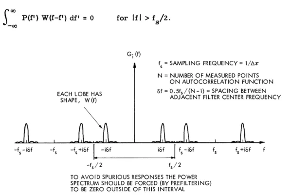
where fs = 1/AT. This result is illustrated in Fig. 3; Gi(f) consists of narrow band-pass regions, each having the shape of W(f), centered at i6f, fs ± i6f, 2fs ± i6f, and

so forth.

It is thus obvious that the autocorrelation spectral measurement system has many spurious responses. It can be seen that these spurious responses will have no effect if the input-power spectrum is restricted (by prefiltering) so that

S

If

I

-O

G; (f)

EACH LOBE HAS

SHAPE, W(f)

J L JLJ

ts = AMILIN, I-KLtLUtN(Y = I/AZ

N = NUMBER OF MEASURED POINTS

ON AUTOCORRELATION FUNCTION 8f = 0.5fs/(N-1) = SPACING BETWEEN

ADJACENT FILTER CENTER FREQUENCY

_lL,

-fs sf -fs -fS+ifL isf isf -Ifs-if fs fs +if f

-f/ 2 fs /2

TO AVOID SPURIOUS RESPONSES THE POWER SPECTRUM SHOULD BE FORCED (BY PREFILTERING) TO BE ZERO OUTSIDE OF THIS INTERVAL

Fig. 3. Filter-array equivalent of the autocorrelation system.

This requirement, a necessary consequence of sampling of the autocorrelation function, is, of course, not required with the filter-method system, since filters without spurious response are easily constructed.

If the requirement of Eq. 27 is met, the terms in which k 0 in Eq. 26 have no effect, and an equivalent set of filter power transfer functions is given by

Gi(f) = W(f-i6f) + W(f+i8f). (28)

Furthermore, if we consider only positive frequencies not close to zero, we obtain

Gi(f) - W(f-i5f). (29)

To summarize, we have shown that the estimation of N points on the autocorrela-tion funcautocorrela-tion (Eq. 23) followed by a modified Fourier transform (Eq. 24) is equivalent to an N-filter array spectral measurement system if Eq. 26 is satisfied. Each method estimates the spectrum over a range of frequencies, B = (N-1)6f = fs/2, with f spacing between points. If the autocorrelation method is used, the spectrum must be zero out-side of this range.

Note that the Gi(f) that can be realized with practical filters is quite different from the equivalent Gi(f) of an autocorrelation system (to the advantage of the filter system). The restriction on W(f) is that it be the Fourier transform of a function, w(T), which must be zero for T > NAT. This restriction makes it difficult to realize an equivalent

Gi(f) having half-power bandwidth, Af, narrower than 2/(NAT) 26f (high spurious lobes result). No such restriction between the bandwidth, Af, and the spacing, 6f, exists for the filter system.

In most filter-array spectrum analyzers, f is equal to Af; that is, adjacent filters overlap at the half-power points. This cannot be done with the autocorrelation method;

6f will be from 0.4 to 0.8 times Af, the value being dependent upon the spurious lobes that can be tolerated. This closer spacing gives a more accurate representation of the spectrum, but is wasteful in terms of the bandwidth analyzed, B = (N-1)6f, with a given resolution, Af. For this reason, it appears that 2 autocorrelation points per equivalent filter is a fairer comparison.

1.5 CHOICE OF THE SPECTRAL-MEASUREMENT TECHNIQUE

We have compared the filter and autocorrelation methods of spectral analysis on a theoretical basis. The major result is that if we desire to estimate N points on the spectrum during one time interval, we may use either an N filter array as in Fig. 2a or a 2N point autocorrelation system as in Fig. 2b. The estimates of the power spec-trum obtained by the two methods are equivalent; there is no theoretical advantage of one method over the other.

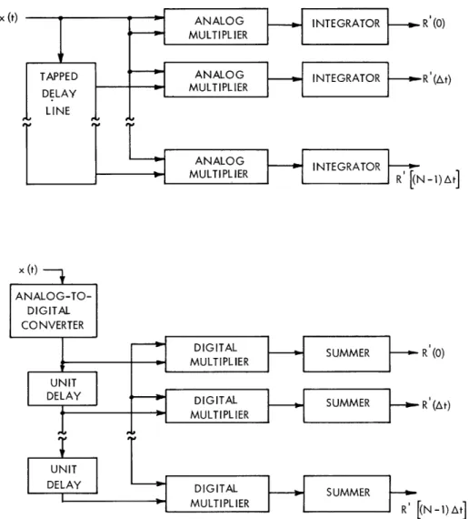
Both methods of spectral analysis can be performed with both analog and digital instrumentation as is indicated in Figs. 4 and 5. In addition, if digital instrumentation is chosen, a choice must be made between performing the calculations

x (t) (0) (At) -1) At] I. I,\ R (0) R (At) (N -1) At] L J

Fig. 4. Analog and digital autocorrelation methods of spectral measurement.

in a general-purpose digital computer or in a special-purpose digital spectrum analyzer or correlator.

The digital filter method4 b shown in Fig. 5 deserves special mention because it is not too well known. The procedure indicated in the block diagram simulates a single-tuned circuit; the center frequency and Q are determined by a and P. The digital simulation of any analog filter network is discussed by Tou.4 The digital filter method will be compared with the digital autocorrelation method below.

A way of classifying spectral measurement problems into ranges where various techniques are applicable is indicated in Fig. 6. The ordinate of the graph is N, the number of significant points that are determined on the spectrum, and the abcissa is the percentage error that can be tolerated in the measurement.

The error in a spectral measurement has two causes: (1) the unavoidable statistical fluctuation resulting from finite duration of data; and (2) the error caused by equipment inaccuracy and drift. The statistical fluctuation depends, through Eq. 20, on the

BANDPASS SQUARE

-x (t) - FILTER LAW INTEGRATOR P (f,)

fo Af DEVICE

_~BADPS

DIGITAL BANDPASS FILTER

r-… - -

-P*(fo )

Fig. 5. Analog and digital filter methods of spectral measurement.

N- B/a NUMBER OF SIGNIFICANT POINTS DETERMINED ON SPECTRUM DURING ONE TIME INTERVAL 1C 1 LINE ANALOG RANGE WITH FEEDBACK OR COMPARISON TECHNIQUE GOOD HYDROGEN-LINE RADIOMETER X 4 108 4x 106 4 x 104 400 REQUIRED Tf PRODUCT

Fig. 6. Ranges of application of several spectral-measurement techniques.

12 x (t) COMPUTER RANGE COMMERCIAL WAVE ANALYZERS 4 x 1010 J

frequency resolution-observation time product, TAf. The value of TAf that is required for a given accuracy is plotted on the abscissa of Fig. 6.

The error caused by equipment inaccuracy and drift limits the range of application of analog techniques, as is indicated in Fig. 6. These ranges are by no means rigidly fixed; exceptions can be found. However, the line indicates the error level where the analog instrumentation becomes exceedingly difficult.

The range of application of digital-computer spectral analysis is limited by the amount of computer time that is required. The line that is drawn represents one hour of computer time on a high-speed digital computer performing 104 multiplications and

10 additions in 1 second. It is interesting that the required computer time is not highly dependent on whether the autocorrelation method or the filter method is programmed on the computer. This will now be shown.

Examination of Fig. 4 reveals that one multiplication and one addition are required per sample per point on the autocorrelation function. The sampling rate is 2B, and 2N autocorrelation points are required for N spectrum points; thus 4NB multiplications and additions per second of data are required. A similar analysis of the digital-filter method illustrated in Fig. 5 indicates that three multiplications and three additions per sample per point on the spectrum are required. This gives 6NB multiplications per second of data. The number of seconds of data that is required is given by solving Eq. 20 for T in terms of the statistical uncertainty, Ap, and the resolution, Af. This gives T = 4/(ApAf) in which the numerical factor a has been assumed to be equal to 2. We then find 16N2/Ap and 24N2/Ap to be the total number of multiplications and

addi-p p

tions required with the autocorrelation method and filter method, respectively. Because of the square dependence on N and Ap, the computer time increases very rapidly to the left of the -hour line in Fig. 6.

Some other considerations concerning the choice of a spectral-analysis technique are the following.

1. If analog instrumentation is used, the filter method is the one that can be more easily instrumented, and, of course, it does not require the Fourier transform. The bandpass filter, squarer, and averager can be realized with less cost and complexity than the delay, multiplier, and averager required for the autocorrelation system. Ana-log correlation may be applicable to direct computation of autocorrelation functions and crosscorrelation functions, but not to spectral analysis.

2. Analog instrumentation is not suited for spectral analysis at very low frequencies (say, below 1 cps), although magnetic tape speed-up techniques can sometimes be used to advantage.

3. Digital instrumentation cannot be used if very large bandwidths are involved. At the present time, it is very difficult to digitally process signals having greater than

10-mc bandwidth.

4. If digital instrumentation, or a computer, is used for the spectral analysis, there seems to be little difference between the autocorrelation and the filter methods if the

RESTRICTIONS ON THE INPUT SIGNAL, x(t): x(t) 1) MUST BE A GAUSSIAN RANDOM SIGNAL

2) MUST HAVE A B.ND-LIMITED POWER SPECTRUM, P(f).O for Ifll B

CLIPPING OPERATION DEFINED AS: CLIPPER

y(t) 1 when x(t O y(t) -1 when x(t) 4

SAMPLING RATE 2 2B * 1/t

SAMPLER

EACH SAMPLE IS A ONE-BIT DIGITAL NUMBER

y(k -t)

ONE-BT FUNCTION OF CORRELATOR DESCRIBED BYt DIGITAL

CORELATOR

j'(n

n.O. Nu-1 -f;(nat)

I

CORRELATION TAKES PLACE FOR T SECONDS.

, (nat) IS THEN READ OUT OF THE CORRELATOR AD IS FED INTO A COMPUTER WHERE THE

FOLLIOWING TAKES PLACE:

NG IS REMOVED BYt (nat] t), IS GIVEN BYt L I'(n&t)w(n&t) I' cos2rTfnAl .~

CORRECTION I(nt) a 8in [P

-P(nat)

-THE SPECTRAL ESTIMATE, p'(:

FOURIER

N-TRANSFORM p'(f) 2at[f(o)(O)+2ZE

THE RESULT, p'(f), IS A S'

p'(f) OF THE POWER SPECTRUM, P(:

HAVE UNIT AREA AND CONVOLVED WITH A FUNCTION

OF BANDWIDTH, f -2B/N.

Fig. 7. The 1-bit autocorrelation method of spectral analysis.

same degree of quantization (the number of bits per sample) can be used. This is evident from the computation of the required number of multiplications and additions. If the autocorrelation method is used, however, only 1 bit per sample is necessary, and the multiplications and additions can be performed very easily. This method will now be discussed.

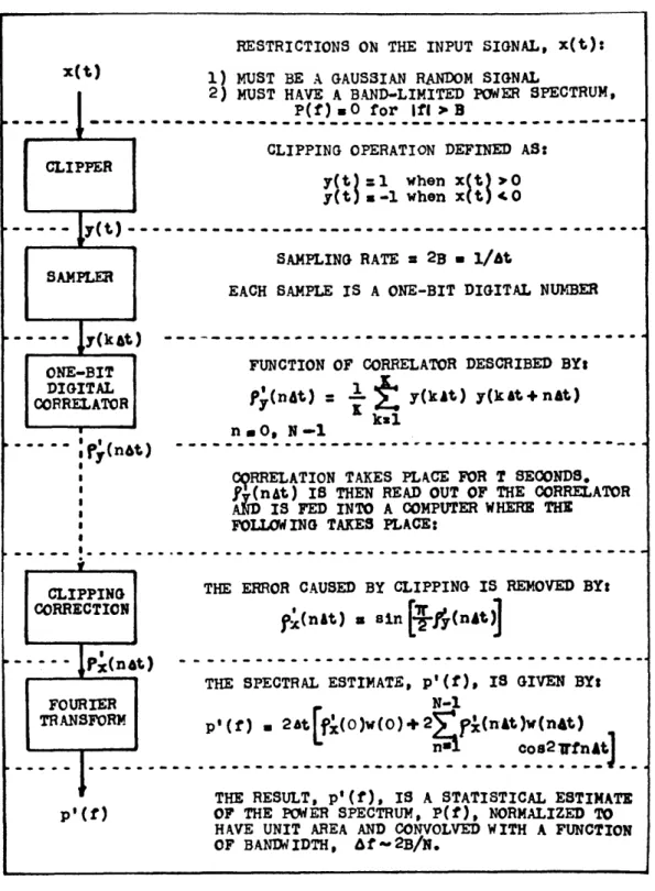
1.6 THE ONE-BIT AUTOCORRELATION METHOD OF SPECTRAL ANALYSIS The one-bit autocorrelation method of spectral analysis as used here is presented with explanatory notes in Fig. 7. Most of the rest of this report will be concerned with the analysis of this system, its application to radio astronomy, and the experimental results obtained with this system.

The key "clipping correction" equation given in Fig. 7 was derived by Van Vleck,5 in 1943. At that time, before the era of digital data processing, the present use of this relation was not foreseen; it was then simply a means of finding the correlation function

at the output of a clipper when the input was Gaussian noise. Its use for the measure-ment of correlation functions has been noted by Faran and Hills,6 Kaiser and Angell,7 and Greene.8 The principal contributions of the present report are: the investigation of the mean and statistical uncertainty (Eq. 20) of a spectral estimate formed as indi-cated in Fig. 7, and the application of this technique to the measurement of spectral lines in radio astronomy.

It should be understood that the spectral-measurement technique as outlined in Fig. 7

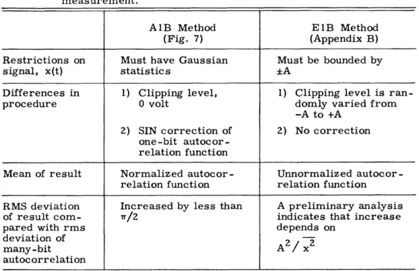
Table I. Comparison of two one-bit methods of measurement.

autoc orrelation-function

A1B Method E1B Method

(Fig. 7) (Appendix B)

Restrictions on Must have Gaussian Must be bounded by

signal, x(t) statistics +A

Differences in 1) Clipping level, 1) Clipping level is

ran-procedure 0 volt domly varied from

-A to +A 2) SIN correction of 2) No correction

one-bit autocor-relation function

Mean of result Normalized autocor- Unnormalized autocor-relation function relation function

RMS deviation Increased by less than A preliminary analysis

of result com- rT/2 indicates that increase

pared with rms depends on

deviation of 2

many-bit A/ x

autocorrelation

applies only to time functions with Gaussian statistics (as defined by Eq. 8). Further-more, only a normalized autocorrelation function and a normalized (to have unit area) power spectrum are determined. The normalization can be removed by the measure-ment of an additional scale factor (such as fo P(f) df). These restrictions do not ham-per the use of the system for the measurement of spectral lines in radio astronomy.

Recently, some remarkable work, which removes both of the above-mentioned restrictions, has been done in Europe by Veltmann and Kwackernaak, 9 and by Jespers, Chu, and Fettweis.1 0 These authors prove a theorem that allows a 1-bit correlator to measure the (unnormalized) autocorrelation function of any bounded time function. The proof of the theorem and the measurement procedure are summarized in Appendix B. A comparison of this procedure with that illustrated in Fig. 7 is outlined in Table I.

It is suggested (not too seriously) that the above-mentioned method of measurement of autocorrelation functions be referred to as the E1B (European 1-bit) method, and the procedure in Fig. 7 as the AIB (American 1-bit) method. Any hybrid of the two pro-cedures could be called the MA1B (mid-Atlantic 1-bit or modified American 1-bit)

method.

II. THE AUTOCORRELATION FUNCTION METHOD OF MEASURING POWER SPECTRA

2.1 INTRODUCTION

The theory of measuring the power spectrum through the use of the autocorrelation function will now be presented. We shall start with the defining equations of the power

spectrum, P(f), of a time function, x(t):

P(f) =2 R(T) e-j2f dT (31)

-00

1 T

R(T) = lim 2T S x(t) x(t+T) dt (32)

T-oo -T

If these equations are examined with the thought of measuring P(f) by directly per-forming the indicated operations, we reach the following conclusions.

1. In practice, the time function is available for only a finite time interval, and thus the limits on T and t cannot be infinite as in Eqs. 31 and 32. Both the time function and the autocorrelation function must be truncated.

2. If the operation of Eq. 32 is performed by a finite number of multipliers and inte-grators, then T cannot assume a continuous range of values. The autocorrelation func-tion, R(T), must be sampled; that is, it will be measured only for = nTr, where n is

an integer between 0 and N-1.

3. If digital processing is used, two more modifications must be made. The time function will be sampled periodically and will give samples x(kZt), where k is an integer

between 1 and (K+N), the total number of samples. Each of these samples must be quantized. If its amplitude falls in a certain interval (say, from xm - A/2 to xm + A/2)

a discrete value (xm) is assigned to it. It will be shown in Section III that the quantiza-tion can be done extremely coarsely; just two intervals, x(kAt) < 0 and x(kAt) > 0, can be used with little effect on the spectral measurement.

These considerations lead us to define the following estimates of the power spectrum and autocorrelation function,

00

P"(f) 2 R"(nAT) w(nAT) e- j2fn AT (33)

n=-oo

K

R"(nA) x(kAt) x(kAt+ nl AT) (34)

k=l

The function, w(nAr), is an even function of n, chosen by the observer, which is zero for Inl > N, and has w(0) = 1. It is included in the definition as a convenient method of handling the truncation of the autocorrelation function measurement; R" (nAT) need

not be known for Inl > N. The choice of w(nAT) will be discussed in section 2.2b. The estimates given by Eqs. 33 and 34 contain all of the modifications (sampling and truncation of the time function and autocorrelation function) discussed above except for quantization of samples which will be discussed in Section III. We shall call these esti-mates the many-bit estiesti-mates (denoted by a double prime) as contrasted with the one-bit estimates (denoted by a single prime) in Section III.

The main objective now will be to relate the many-bit estimates, P"(f) and R"(nAT), to the true values, P(f) and R(nAT). Many of the results will be applicable to the dis-cussion of the one-bit estimates; other results were found for the sake of comparison with the one-bit results.

It is assumed that x(t) is a random signal having Gaussian statistics. The estimates P" (f) and R"(nAT) are therefore random variables, since they are based on time aver-ages (over a finite interval) of functions of x(t). The particular values of P"(f) and R(nAT) depend on the particular finite-time segment of x(t) on which they are based.

The mean and variance of P"(f) and R"(f), for our purposes, describe their prop-erties as estimates of P(f) and R(nAT). The mean, R"(nAT), of R"(nAT), is easily found to be

K

R"(nAT) = - x(kAt) x(kAt+ nlAT) (35)

k= 1

R" (nAT) = R(nAT). (36)

Here we have made use of the fact that the statistical average of x(kAt) x(kAt+lnl T) is simply R(nAT). R" (nAT) is called an unbiased estimate of R(nAT).

The mean of P"(f) is also easily found by taking the statistical average of both sides of Eq. 33 and using Eq. 36. Defining P *(f) as the mean of P"(f), we find

00

P *(f) P"(f) = 2AT

£

n=-oo

If it were not for the sampling and truncation of R(T), P (f) would simply be equal to P(f), and hence P" (f) would be an unbiased estimate of P(f). The relationship of P *(f) to P(f) is discussed below. The variances of P" (f) and R" (nAT) will also be found.

Much of the material presented here is contained in a different form in a book by Blackman and Tukey. 11 For the sake of completeness this material has been included here. An extensive bibliography of past work in this field is listed in this book.

2.2 MEAN OF THE SPECTRAL ESTIMATE a. Relation of P *(f) to P(f)

It has been shown that the mean, P *(f), of the many-bit spectral estimate is given (Eq. 37) as the Fourier transform of the truncated and sampled autocorrelation function.

In Section III we shall find that the mean of the one-bit spectral estimate is equal to P *(f) divided by a normalization factor. It is thus quite important that the relationship between P *(f), the quantity that we estimate, and P(f), the true power spectrum, be well understood.

This relationship is found by substituting the following Fourier transform relations for R(nAT) and w(nAT) in Eq. 37.

R(nT) = P(a) eZra j nA da (38) -00 w(nAT) = W(P) e d[ (39) -00o The result is oo

P (f) = , a P(a) W(f-a-ifs) da, (40)

i=-00 00

where fs = /AT, and we have made use of the relation

00 co

Ar Ej jzT2nAT(a+p-f) = 6(a+p-f+ifs).

n=-oo i=-oo

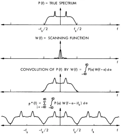
Equation 40 not only specifies P *(f) in terms of P(f), but it should also be con-sidered as the general definition of the * operator which will be used in this report. This operation is described in Fig. 8. Two modifications of P(f) are involved; the first is a consequence of truncation of the autocorrelation function and the second is a conse-quence of sampling of the autocorrelation function:

1. The spectrum is convolved with W(f), a narrow-spike function of bandwidth, f fs/N. This convolution should be considered as a smoothing or scanning operation. Features in the spectrum narrower than Af are smoothed out.

2. The smoothed spectrum is repeated periodically about integer multiples of fs If the convolution of P(f) and W(f) is zero for If I > fs/2, then Eq. 40 simplifies to

p*(f) =

S

In practice fs will be chosen to be twice the frequency at which the smoothed spectrum is 20 db below its midband value. In this case, little error (<1 per cent in the midband region) occurs because of sampling, and P (f) can be considered as a smoothed version of P(f). If P(f) does not change much in a band of width Af, then

P *(f) P(f). (42)

P (f) = TRUE SPECTRUM

-fS/2 fs/2 f

W(f)= SCANNING FUNCTION

f

co

CONVOLUTION OF P(f) BY W(f) = P(a) W(f-a)da

-co

f

aO D

p*(f) = C P(a) W(f-a- fs)da i = -c -O

f_S/2 fs

Fig. 8. Effect of sampling and truncation of the autocorrelation function. The quantity P (f) is the mean of a spectral measurement performed with an autocorrelation system.

The relationship between P (f) and P(f) should be quite familiar to those versed in the theory of antenna arrays (or multiple-slit diffraction theory). The function

00

2 W(f-ifs) is analogous to the antenna field pattern of a line array of N point sources

i=-oo

with amplitudes weighted by w(nAT). b. The Weighting Function, w(nAT)

The shape of the spectral scanning function, W(f), is determined by the choice of

its Fourier transform, the autocorrelation weighting function, w(nA-r). The weighting function can be arbitrarily chosen except for the following restrictions:

w(O) = 1 =

-00

w(nA-r) = w(-nTr)

w(nA-) = 0 for Inl > N.

The choice of w(nAT) is usually a compromise between obtaining a W(f) with a narrow

W(f) df (43)

(44) (45)

- v~~~~~~ w | b

I I I I i UNIFORM WEIGHTING C \/WG HTN CS WEIGHTING , 11I I~.., -10 -20 -30 0 0.5 1 N f/f 0.1 0,01 0.001 1.5 2 2.5

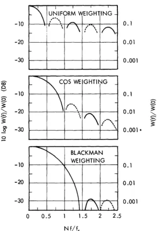
Fig. 9. Three scanning functions that result from the uniform and cosine weighting functions (after Blackman and Tukeyl 1) . The broken lines indicate that W(f) is negative. See also Table II.

main lobe and high spurious lobes, or a W(f) with a broadened main lobe and low spu-rious lobes.

This problem is a common one in antenna theory and optics. The "optimum" w(nAT) obviously depends on some exact specification of the performance of W(f). This crite-rion will usually depend on the particular measurement that is being made. Some weighting functions that appear to be optimum in some sense are: the uniform weighting function (to be discussed below) which gives a narrow main lobe; the binomial weighting function (Kraus 2 ) which gives no spurious lobes; and the Tchebycheff weighting function (see Dolph 1 3) which gives equal spurious lobes.

It appears that little can be gained by making a very careful choice of w(nAT). Blackman and Tukey 1 describe five weighting functions; three of these should be adequate for most applications and are given in Table II and Fig. 9. The cos weighting function appears to be a good compromise for most spectral-line observations in radio astronomy; the uniform weighting function gives sharper resolution, whereas the Blackman weighting function gives low (-29 db) spurious lobes. -10 -20 -30 0.1 0.01 0.001 0.1 vO 0.01 \ 0.001· S o -10 -20 -30

I 's4 aP _ c

A

0b

-'

a

4

I

-z

IL

II

4

17

f

i

I

I

'

Ib

I

j

i

c. Some Useful Properties of P *(f)

Some useful relations between P *(f) and R(nAT) can be obtained by using conven-tional Fourier techniques. These relations are all derived from Eq. 37:

oo

P*(f) = 2AT R(nAT) w(nAT) e j if nAT

n=-oo

This equation, with P (f) and R(nAr) replaced by different quantities, will often occur, and hence, the results of this section will also apply to the following quantities which replace P *(f) and R(nAT):

P"(f) and R"(nAT) The many-bit estimates of P *(f) and R(nAT)

p"(f) and p"(nAT) Normalized many-bit estimates that will be discussed below p*(f) and p(nAT) Normalized quantities analogous to P *(f) and R(nAT)

p'(f) and p'(nAT) Normalized one-bit estimates that will be defined in Section III. If Eq. 37 is multiplied by e j2rf kAT and the result is integrated from zero to fs/2,

we find

R(nAT) w(nAT) = §s P*(f) cos 2f nAT dT. (46)

This is analogous to the inverse transform relationship (Eq. 14) between R(T) and P(f). Setting n = 0 in Eq. 46 and T = 0 in Eq. 14 gives

R(0) = s / 2 P*(f) df (47)

and

R(0) = P(f) df, (48)

where R(O) is the total time average power.

The Parseval theorem for P (f) can be derived by substituting Eq. 37 for one P *(f) in the quantity f/2 P (f) P* (f) df. The result is easily recognized if Eq. 46 is used. The result is

0 /2 00

, [P*(f)] df = 2AT E R 2(nA) w (nAT) (49)

n=-oo

which is sometimes useful.

2.3 COVARIANCES OF MANY-BIT ESTIMATES OF THE AUTOCORRELATION FUNCTION AND POWER SPECTRUM

2 2

We shall examine the covariances pm(flf2) and arRm(n,m) of estimates P"(f) and R"(nAT) (defined in Eqs. 33 and 34), of the power spectrum and autocorrelation function,

respectively. These estimates are based on many-bit (or unquantized) samples of the time function as opposed to estimates based on one-bit samples that are the major topic of this report. The calculations of the covariances in the many-bit case are included for the sake of comparison. The following discussion applies to both many-bit and one-bit cases.

a. Definitions: Relation of the Spectral Covariance to the Autocorrelation Covariance

The covariance of the power spectrum estimate is defined as

Pm(f lf ) [P (fl)_p*(fl)][P (f2)p*(f) ] (50)

crm(1 ) P"(fl) P"(f2) - P (fl) P(f2 ) (51)

A special case arises when fl = f2 = f and the covariance becomes the variance, 2pm(f) .

The positive square root of the variance is the rms deviation, arpm(f). The variance and rms deviation specify the way in which P"(f) is likely to vary from its mean, P *(f). The covariance also specifies how the statistical error at one frequency, fl, is corre-lated with the statistical error at another frequency, f2.

The definition of the autocorrelation covariance is quite similar. 2

(r,(nm) [R(nAT)- R(n T)][R " I(nAT)-R(nAT)] (52)

2

a'Rm(n,m) = R"(nAT) R"(nAT) - R(nAT) R(nAT) (53)

and the meaning of the autocorrelation variance and rms deviation follow accordingly. The spectral covariance or variance can be expressed in terms of the autocorrelation covariance by substitution of Eqs. 33 and 37 in Eq. 51. This gives

22 2 -j 2 AT(nfl+mf2)

pm(flf2)= 4AT 2 a '2 (nm) w(nAT) w(mAT) e

*

PMf = 1, 2 Rm

n=-oo n=-oo

Our first step will be to calculate the autocorrelation covariance. This is not only needed for the calculation of the spectral covariance, but is also of interest on its own

accord.

Note that the autocorrelation covariance is required to calculate the spectral vari-ance or covarivari-ance; the autocorrelation varivari-ance is not sufficient. The integrated (over frequency) spectral variance can be expressed in terms of the autocorrelation variance

summed over the time index, n. This relation is found by integrating both sides of Eq. 54 (with f2 = f1) from 0 to fs/2. The result is

s 2 2

$

)

n=-co

b. Results of the Autocorrelation Covariance Calculation 2

The covariance, orRm(n,m), of the many-bit autocorrelation function estimate is cal-culated in Appendix C; the results will be discussed here.

The covariance, expressed in terms of the autocorrelation function, is found to be K

a'R2(n,m) = 1 E [R(iAt+ I n I AT- I m l AT) R R(iAt+ n

I

A plot of a typical autocorrelation function and its rms deviation, Rm(n), is given in Fig. 10.

It is informative to investigate the autocorrelation variance (n=m) in two limiting cases:

Case 1

Suppose that At is large enough so that

R(iAt) = 0 for i 0. (57)

Equation 56 then reduces to

2 R2(0) + R(nAT)

Rm(n) = K (58)

The condition of Eq. 57 implies that successive products, x(kAt) x(kAt+ InAT ), which go into the estimate of the autocorrelation function, are linearly independent. There are K such products and the form of Eq. 58 is a familiar one in statistical estimation problems.

In order to minimize the variance, K should be made as large as possible. If the duration, T, of the data is fixed, then the only recourse is to reduce At = T/K. As At

is reduced, a point will be reached where Eq. 57 is not satisfied. The minimum value of At which satisfies Eq. 57 is equal to 1/2B if x(t) has a rectangular power spectrum extending from -B to B, and if AT is set equal to 1/2B. The variance at this value of At is

2 R2(0) + R (nAT)

ORm(n) = 2BT '

where R(nAT) = 0, n 0 for the rectangular spectrum with AT = 1/2B.

The next example will illustrate the point that the variance cannot be reduced further by reduction of At beyond the point required by Eq. 57.

R(O)

I

i

I

Fig.B 10. An autocorrelation function and its transform, the power

Fig. 10. An autocorrelation function and its transform, the power spectrum. The form of the rms deviation is indicated. Note that -pm(f) is proportional to P(f) (except near f = 0), whereas Rm(T) is nearly constant.

Case 2

Suppose that At - 0 and K - o in such a manner that KAt = T is constant. The case of continuous data (analog correlation) is approached and Eq. 56 (with n = m) becomes

rR2 T() [R2(t)+R(t+nAT) R(t-nAT)] dt. (60)

Rm - T

If again we take the case of a rectangular spectrum between -B and B, Eq. 60 gives

2 R 2(0) + R2(0) (sin 4TB nAT)/(4rBnAT)

aRm(n) = 2BT (61)

This result, with AT = 1/2B, agrees exactly with Eq. 59. Thus, reducing the time-function sampling interval At from 1/2B to 0 has had no effect on {Rm(n) for the case of a rectangular spectrum.

Examinations of Eqs. C. 8 and C. 11 in Appendix C give more general results. These equations show that both the autocorrelation variance and the spectral variance do not change for values of At less than 1/2B if P(f) = 0 for f > B.

c. Results of the Spectral Covariance Calculation 2

The spectral covariance, pm(fl f2), is calculated in Appendix C with the following result.

Pm ₂ ,f )

--- n

fPm('f2) T P (f) W(f+fl) [W(f+f2)+W(f-f 2)] df. (62)

It has been assumed that: (a) the signal has Gaussian statistics; (b) both P(f) and W(f) are smooth over frequency bands of width /T; (c) the spectrum smoothed by [or convolved with] W(f) is zero for frequencies greater than B; (d) both the time-function sampling interval, At, and the autocorrelation-function sampling inter-val, AT, have been chosen equal to 1/2B; and (e) Eq. 62 is valid only for If l and If2 less than B.

The manner in which the spectral estimate covaries is observed in Eq. 62. If f and f2 are such that W(f+f1) and W(f±f2) do not overlap, then pm(fl f2) = 0. In other

words, the statistical errors at two frequencies separated by more than Af, the band-width of W(f), are uncorrelated. This result might have been expected from the analogy with the filter-array spectrum analyzer discussed in Section I.

The spectral variance (fl = f2) can be put in a simpler form if some further

approxi-mations are made. It can be seen that at fl = f2 = 0 the variance becomes

2 2 2 2

G Pm - rT _ p2 (f) W2(f) df, (63)

-00

while, for fl = f2 >>Af, we obtain

Pm(f1) = p(f) W2 (f+f1) df. (64)

00

In the following discussion we shall assume that f is positive and not close to zero so that Eq. 64 applies.

If the spectrum is smooth over bands of width f, then P(f) can be taken out from under the integral sign in Eq. 64 to give