A dynamic model of competition

(1)

A Dynamic Model of Competition

by

Matthew George Escobido

M.S. Mechanical Engineering, Toyohashi University of Technology, 1998 B.S. Physics, University of the Philippines, 1993

Submitted to the System Design and Management Program

in partial fulfillment of the requirements for the degree of

Master of Science in Engineering and Management

at the

MASSACHUSETTS INSTITUTE OF TECHNOLOGY

January 2009

JUN 0 3 2009

(2)

(3)

A Dynamic Model of Competition

by

Matthew Escobido

Submitted to the System Design and Management Program on January 16, 2008 in partial fulfillment of the requirements for the degree of Master of Science in Engineering and Management

Abstract

The Lotka-Volterra competition model has been extensively used in the study of tech-nology interaction. It looks at the growth rate of a certain parameter of the interacting technologies through coupled nonlinear differential equations. The interaction is then modeled as a competition with a constant competition coefficient that adversely af-fects the growth rate. Various studies, however, have suggested that the interaction is not only pure competition and that other interactions are possible. These suggestions have remained mostly conceptual and descriptive - lacking a definite mathematical form of the interaction that can accommodate the suggested variations and the specif-ic implspecif-ication of those variations.

This thesis presents a specific form of the competition coefficient that depends on the cost and benefit of the competition to a particular technology. The cost and benefit functions are patterned after density-dependent (size) interactions in ecology. The re-sulting competition coefficient is not a constant but varies as the density of the com-peting technologies changes. Based on the variable coefficient, we extracted steady states and derived conditions of stability to analyze the dynamics of the competition. Results show that the model can provide a richer set of possibilities compared to the constant coefficient. It accommodates different modes of interactions such as symbi-osis and predator-prey aside from pure competition in the steady state coexistence be-tween technologies. It allows for shifts from one mode to another during the evolution of the technologies. Lastly, it provides modifications to strategies meant to achieve "winner-take-all" scenario coveted in business.

Thesis Supervisor: James M. Utterback

Title: David J. McGrath jr (1959) Professor of Management and Innovation and Professor of Engineering Systems

(4)

(5)

Acknowledgments

"If I have been able to see further, it was only because I stood on the shoulders of giants."

- Isaac Newton

This thesis would not be possible without the support, encouragement, and construc-tive suggestions of Prof. James Utterback. His expertise in management and technol-ogy dynamics and willingness to help have kept me on course - ably guiding as I thread unknown paths, and gently prodding when the course runs dry.

I was fortunate to have resources that satiated my curiosity in nonlinear phenome-na and ecological models. The books by Prof. Steven Strogatz (nonlinear dyphenome-namics) and Prof. James Murray (mathematical biology) stood out for being comprehensive and readable. It is rare that books of these types could teach by just reading them!

Deepest gratitude also goes to the people behind the System Design and Manage-ment (SDM) program: Pat Hale for providing the opportunity to be part of the 2008 cohort; Bill Foley, Amy Jordan, Dave Schultz and Chris Bates for always looking out for us; fellow cohorts notably Sy, Cynthia, Dev, Amar and Ben for the long hours working together and the priceless friendship!

I want to acknowledge as well the grants provided by SDM and PAEF (Philippine-American Foundation) and the support of my family and friends that made studying at MIT a little affordable. The efforts of my parents and siblings, Eileen Valdecanas, Dr. Esmeralda Cunanan, and Naoko Ito are greatly appreciated.

Last but definitely not the least, I want to thank my wife Eileen and son Kyle for their sacrifices while I'm away and their incessant encouragement that made all these possible. This thesis is dedicated to them.

(6)

List of Figures

Figure 2-1. Equilibrium values for N as a function of the competition coefficient c ..23

Figure 2-2. Basin of attraction for (N1, 0) ... ... 24

Figure 2-3. Evolution of the competing technologies for different initial conditions Nlo and N2o. (Parameter values: r =r2=0O.1, K1 =K2=2, c12=C21=0.15) ... 25

Figure 2-4. Competition coexistence steady state value. (a) Time evolution (b) Phase plane nullclines. (Parameter values: rl=r2=0.1, K =K2=2, c12=c21=0.05)...26

Figure 2-5. Strategy options and resulting steady state values for technologies T1 and T2 based on fractional growth rate f, and carrying capacityfk... 28

Figure 3-1. Predator-prey sample dynamics: (a) Technologies coexisting; (b) Only N1 Survives. Parameter values: ri=r2=0.1, K₁=K2=2, c12=C21=C ... 35

Figure 3-2. Predator-prey coexistence steady state value. (a) Time evolution (b) Phase plane nullclines. (Parameter values: rl =r2=0.1, K=K2 =2, c12=C21=0.05)...36

Figure 3-3. Symbiosis sample dynamics: (a) Technologies coexisting ( c12c21 < rlr2); (b) Unbounded growth. Parameter values: rl=r2=O.1, K1=K2=2, C12= C21= C ... ... ... . ... .. 38

Figure 3-4. Symbiosis coexistence steady state value. (a) Time evolution (b) Phase plane nullclines. (Parameter values: r]l=r2= 0.1, K =K2=2, cl2=C21= 0.05) .... 38

Figure 4-1. Varying competition coefficient (solid line) and constant coefficient (dashed line)...43

Figure 4-2. Benefit function and associated parameters ... 47

Figure 4-3. Cost function and associated parameters ... ... 48

(10)

Figure 4-5. Comparison of Winner-Take-All scenario: (a) Constant coefficient (b) Variable coefficient (c) Variable coefficient - modified. Parameter values:

rl=r2=0.1, K=K2=2 ... 53

Figure 4-6. Sample nullclines and coexistence steady states for variable coefficient .55 Figure 4-7. Lotka-Volterra interaction framework coexistence steady states for constant coefficient ... 56

Figure 4-8. Sample of possible modes of coexistence for the variable coefficient ... 57

Figure 4-9. Evolution of the competition coefficient. Parameter values: rI=r2=0.1, K1=K2=2, c =C2 = 1, 31=132=0.5, y7=2=6.9 . .... . . . .. . . 58

Figure 4-10. Multi-mode interactions in the evolution of competition. Parameter values: rl=r2=0.1, K1=K2=2, a1=z2= 1, 31=132=1.5, 71=72=5 ... 59

Figure A -0-1. N ullclines... ... 67

Figure A-0-2. Stability classification of equilibrium points... ... ... 68

Figure A-0-3. Phase portrait ... 69

(11)

List of Tables

Table 2-1. Equilibrium points and stability conditions: Competition model ... 22

Table 2-2. Competition equilibria and stability: rl = r2 = r; K1 = K2 = K; c12 = c21 = c ... 23

Table 2-3. Stability condition for mature technology -new technology competition .27 Table 3-1. Mode of interaction based on the combination of the signs preceding the interaction coefficient... .. ... ... 31

Table 3-2. Equilibrium points and stability conditions: Predator-prey interaction ... 34

Table 3-3. Equilibrium points and stability conditions: Symbiosis ... 37

Table 3-4. Lotka-Volterra classification framework based on the sign of the com petition coefficient... ... 39

Table 4-1. Equilibrium points and stability conditions: Variable Competition ... 51

Table 4-2. Comparison of Winner-Take-All Conditions ... 52

Table 4-3. Comparison of Coexistence Steady States ... 54

(12)

(13)

Chapter 1 Introduction

"It is not the strongest of the species that survives, nor the most intelligent... but the one most responsive to change."

-Attributed to Charles Darwin

1.1 Competition Between Technologies

The dynamics of interaction between or among technologies have been discussed ex-tensively in the literature .The details of the dynamics can be overly complicated

-with numerous players, each able to pursue unique strategies at different time frames. Different models have explained certain aspect of the dynamics of interaction. These models range from linear ordinary differential equations to coupled nonlinear partial differentials equations, discrete to continuous models and have yielded analytical and computational results.

Many of these models treat the interaction as competition where two or more technologies compete for the same general market and in the process inhibit each oth-er's growth. Prominent among these models is the Lotka-Volterra competition model which will be the subject of this thesis. It considers the growth rate of a particular va-riable describing the evolution of the technology. This vava-riable can be the number of

See for instance (Abernathy & Utterback, 1978), (Utterback & Suarez, 1993), (Christensen, Innovator's Dilemma: When New Technologies Cause Great Firms to Fail, 1997), (Weil & Utterback, 2005)

(14)

units of the technology sold or the market size of the technology among other things. The diffusion of the technology as denoted by the growth rate of this variable is dri-ven by its intrinsic growth rate (or growth rate in the absence of competition) but li-mited by its finite carrying capacity and by the extent of competition with other tech-nologies. The interplay among these parameters is presented as coupled differential equations. The solution to these Lotka-Volterra equations synthesizes the dynamics of the interaction between or among the technologies.

The Lotka-Volterra competition model has been shown to be sufficiently general to encompass different kinds of models. Linear, exponential, Pearl, Gompertz, substi-tution models and oscillatory behaviors can all be matched by the competition model2. It is capable of depicting a wide range of dynamic behaviors such as the S-curve, network effects and oscillatory behaviors. It has been used to model different technol-ogies replacing or substituting another technology - lead-free cans replacing soldered cans, tufted carpets replacing woolen carpets, ball point pens replacing fountain pens and nylon tire cord replacing rayon tire cord3

For all its successes, the model has been criticized by ecologists for the constancy of the competitive interaction as given by its constant coefficient4. An effort towards addressing this shortcoming is the introduction of the functional response in the inte-raction depending on the density (size of the population) of the competitors5. While acceptable in ecology, the modification, however, fall short in explaining certain technology interactions and business developments. The functional response can ad-dress the extent of competition but does not change the nature of interaction (e.g. still pure competition or predator-prey). This makes sense from the perspective of ecology where the lions eat the zebras and never vice-versa. It is, however, limiting in under-standing technology interactions where the roles in the competition may change in time.

2 _{(Porter, Roper, Mason, Rossini, Banks, & Wiederholt, 1991)} 3 (Farrell, 1993)

4 (Abrams, 1980)

(15)

Several researchers have presented examples where interaction between technolo-gies is not necessarily purely competitive. Instances where one technology has a posi-tive effect on the growth rate of another technology (symbiosis), or one technology benefits at the expense of the other (predator-prey) have been cited6. The symbiotic interaction between computer software and hardware is a classic example of the for-mer. The substitution of the bias ply-tires by radial-ply tires illustrates the latter.

Within the context of the Lotka-Volterra equations, the interactions can be classi-fied to different modes depending on how it affects the growth rates of the interacting technologies. This classification is facilitated by changing the sign before the interac-tion term (which is assumed to be always positive). Pure competiinterac-tion would have negative signs for both (negative effect on both); predator-prey has a positive

(preda-tor - positive effect) - negative (prey - negative effect) combination; and symbiosis

has both positive signs (positive effect for both)7.

Not only are there different interactions possible aside from pure competition, these interactions can change from one mode to another in time. These temporal shifts can manifest in the technologies themselves, in the structure of the companies or in the industries for which these technologies are a part of. Take for instance the devel-opment of the hard disk drive for the personal computer markets_{. The incumbent}

5.25-inch disk technology offered higher capacity while the 3.5-inch alternative was smaller and more energy efficient. The former was used in the mainstream desktop segment while the latter served the emerging market for portable computers. Thus, the two technologies were initially growing together but each limited to serving consum-ers in a different market segment. In time, however, the performance of the 3.5-inch drives had expanded from the portable segment to capture the low-end of the desktop segment.

Within the Lotka-Volterra context, such development can be modeled as symbiosis and later predator-prey. The mechanism of switching from one mode to another, for example from initially symbiotic relationship to eventually predator-prey, is, however,

6 _{See for instance (Pistorius & Utterback, A Lotka-Volterra Model for Multi-mode Technological} 7 This classification scheme is borrowed from ecology (Odum, 1953)

(16)

lacking. What is needed is a definite mathematical form of the interaction that can ac-commodate the suggested transition.

Efforts have been made to consider variations in the Lotka-Volterra model. Varia-tions of the parameters by considering sinusoidal dependency have been implemented to approximate phenomenological substitution models9. Effects of stochastic exten-sions of the equations were also studied1o. These variations, though important, are confined to a particular mode. Examples beyond periodic variations or random fluctu-ations have been made to suggest a more dynamic pattern of shifts in the relation be-tween two technologies from one mode of interaction to another' 1

This thesis provides a mechanism that would allow for the shifting of the relation between competing technologies. It presents a specific form of the competition coef-ficient that depends on the cost and benefit of the competition to the technologies in-volved. The cost and benefit functions are patterned after density-dependent (size) interactions in ecology. The resulting competition coefficient is not a constant but va-ries as the density of the competing technologies changes.

Based on the variable coefficient, we derived conditions of stability to analyze the dynamics and the implications of the competition. We compare the results to the case of constant coefficients. The results indicate that the model can provide a richer set of possibilities and a more dynamic model of competition. It presents different modes of coexistence and accommodates coexisting steady states with values larger than its car-rying capacity. It allows for different forms of interactions such as symbiosis and pre-dator-prey aside from pure competition during the evolution of the technologies. Last-ly, it provides modifications to strategies meant to achieve "winner-take-all" scenario coveted in business12

9 (Bhargava, 1989)

10 (Solomon, Richmond, Biham, & Malcai, 2004)

" See for instance (Pistorius & Utterback, Multi-mode Interaction among Technologies, 1997), (Modis, 1997)

(17)

1.2 Organization of the Thesis

Modeling the dynamics of a system of competing technologies involves three main tasks: defining the mathematical functions that govern the appropriate variables of the system; (2) collecting experimental data on these variables of the system; and (3) de-ciding on the values for the adjustable parameters in the mathematical functions of the model. The first two tasks are independent and would be sufficient for a separate the-sis. They set the stage for the third task to provide specific predictions that can be ex-tracted from the given mathematical formalism and the collected data set.

Given the time constraint within the SDM program, a conscious effort was made to focus on the first task - defining the mathematical form of the model that would best illustrate the competition between technologies. To go about this, we present the results of the current competition model to highlight the need for a new model and compare the results later. Chapter 2 presents the dynamics of the Lotka-Volterra com-petition model and its steady state (long-term) implications. The Lotka-Volterra framework, however, allows other interactions aside from pure competition. Chapter 3 discusses these interactions and serves as a reference of possible behavior that can be covered in our new competition model.

The gist of the thesis is in Chapter 4 where we define the specific form of the competition coefficient that can accommodate different types of interactions. The re-mainder of the chapter attempts to deduce the dynamics of the resulting model. It compares and contrast the results derived in Chapter 2 and Chapter 3. Chapter 5 con-cludes the thesis with a summary of the results and implications of the model. An ef-fort was exerted to cover in general terms the possible next steps that need to be taken for the remaining tasks.

(18)

(19)

Chapter 2 Lotka-Volterra Competition Model

"Winning isn't everything; it's the only thing."

- _{Henry Russell ("Red") Sanders}

In this chapter, we are going to present the Lotka-Volterra competition model and re-view the implications of the model. We will highlight the attributes of the model that we would modify later, and cast the results of the model in a form that would facili-tate comparison in succeeding chapters.

2.1 Competition Model

The Lotka-Volterra competition model looks at two or more technologies competing for the same general market and inhibiting each other's growth' 3. It considers the growth rate of a particular variable N1 describing the evolution of the technology T1.

This variable can be the number of units of the technology sold or the market size of the technology. In the absence of competition, it is assumed that N1 grows

exponen-tially with intrinsic growth rate rl. The increase, however, is limited by its carrying

(20)

capacity denoted by K1 resulting in a logistic growth'4. The competition with another technology T2 decreases further the growth by an amount proportional to the

interac-tion of the defining variable of T1 with T2, i.e. oc N1N2. The proportionality constant is

denoted as the competition coefficient c12 on N1 due to N2. As such c12 is the rate at

which N1 loses in the competition with N2.

Similarly, T2would be described by the growth rate of N2 with intrinsic growth

rate of r2, carrying capacity K2 and inhibited by competition with T1 at a rate of c21.

With these attributes and parameters, the competition model then takes the form:

dN 1 N C12 dN1 = r Nj -- N) NN2 dt K, K1 (2.1) dN2 = N2 C21 dt K2 K2

As originally presented, the parameters ri, Ki, cij (i,j = 1,2) are positive constants. In

Chapter 4 we will make the case that the competition coefficient is not a constant, and specifically present a form that can shift from negative to positive values and vice-versa.

N.

Note that it is possible to rescale the parameters in (2.1) (e.g. ni = , i = rit) to

reduce the number of parameters and simplify the equations 15. However, we purposely retained the explicit form of the equations since the parameters involved have real physical significance as can be seen in the succeeding discussion. Note also that the competition coefficient is scaled by the carrying capacity (i.e. K) so that the results

would be dimensionally consistent with the growth rate.

14 _{(Verhulst, 1838)}

(21)

2.2 Critical Dynamics

The Lotka-Volterra competition model is a nonlinear differential equation with no simple closed-form analytic solution. However, one can completely understand the dynamics of the model by investigating its evolution in the phase plane. To go about this, we introduce some concepts that would be needed in our analysis. These con-cepts would be used again when we present other models of technology interactions. The details of these concepts are given in Appendix A.

These concepts include the equilibrium point, steady state, eigenvalues and sta-bility. The points where there is no change in the growth rates of the pertinent varia-ble N correspond to a steady state solution. These equilibrium points can be obtained by equating the Lotka-Volterra equations to zero (i.e. Nl = 0, N2 = 0) to yield the

equilibrium. One can think of the equilibrium points as the pay-offs and the steady state solution as the long-term end state of the competition. Stability (or asymptotic stability)16 is a characteristic of a system where small perturbations around the equili-brium points have only small effects and vanishes for long periods of time. The ei-genvalue (denoted by the symbol 2) provides a means of classifying the stability of our system given the equilibrium points. For our purpose, we look for pay-offs of sta-ble, lasting end states as opposed to transitory states. A necessary and sufficient con-dition for stability is that the real part of the eigenvalue Re(A) < 0.

For the competition model, the equilibrium points, eigenvalues and conditions for stability are given in Table 2-1:

16 _{We differentiate stability (asymptotic stability) with neutral stability. In the former, the perturbations}

vanish and the system is attracted back to the equilibrium point after long time period. In the latter, the per-turbations permanently disturbed the system, remaining close to the original equilibrium point but not at-tracted to it.

(22)

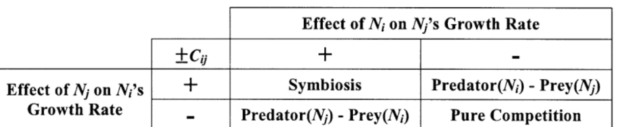
Table 2-1. Equilibrium points and stability conditions: Competition model

Equilibrium Points Eigenvalues Stable if

(N*, N2) (0,0) A1,2 = 1, r2 Never (K, 0) c2 1K1 C21 > 2K2 ;12 =2 K2 Kr /1 = -r2 (0, K2) c1 2K2 C1 2 > LK 12 =r 1 K2 -B + VB 2 - 4C r2(Kr 1-cz1 2K2) 1 2 2 rTir2 - C12C21

B=

r 2 N ri(K2r2 - c2 1K1) K K2 2 C1 2C2 1 < r2 rl 2 - C12C21 C= 1 2 - C1 2C21 NN

2.2.1 Case 1: Technologies are Similarly Situated

To understand the dynamics, let us consider the case where the competing technolo-gies are similarly situated. This would correspond to two competing technolotechnolo-gies with similar growth attributes and capacity potential. This means that ri = r2 = r; K1 =

K2 = K and the competition coefficient is symmetric17 i.e. c12 = c21 = c. We want to

examine now their dynamics as their competitive interaction increases. The equilibrium points and stability conditions are given by Table 2-2:

17 In general, the competition coefficient is asymmetric, i.e. cyij cji. For example, with their difficulty in adapting threatening technology, established technologies do not threaten emerging technologies as much as other emerging technologies would.

(23)

Table 2-2. Competition equilibria and stability: r, = r2 = r; K1 = K2 = K;c12 = C21 = C

Equilibrium Points Stable if

(NI , N2*) (0,0) Never (K, 0) _{c > r} (0, K) c 2 r C Kr _Kr c<r r + c'r + c)

For a given intrinsic growth rate r and competition coefficient c, the stability of the equilibrium points would require the competition coefficient c to be less than or greater than the growth rate r. It can be that for small values of c, c < r which would

(Kr Kr \

make the equilibrium point r+c , stable. This means that both technologies

coex-\r+c r+c' Kr

ist with equal steady state values --. As the competition heats up, c increases,

even-tually becoming greater than the growth rate r. This makes the equilibrium points

(K, 0) and (O,K) stable. These equilibrium points, however, meant the extinction of the

other technology. This behavior is shown in the graph below:

I

V

orN2

N, and2

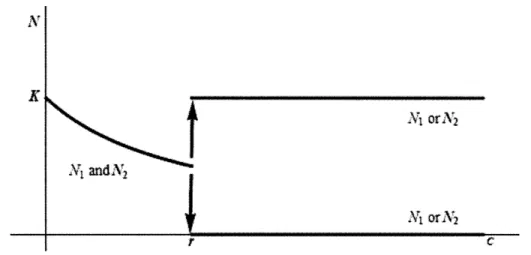
Figure 2-1. Equilibrium values for N as a function of the competition coefficient c

As Figure 2-1 shows, there is a sudden discontinuous transition at c = r. For low

(24)

Howev-er, for high competition, the market transitions into a "winner-take-all market"18

con-dition in which one competitor grabs all market share, whereas the other gets nothing. Though we have presented only two competing technologies here, the condition has been shown to persist also for the model with more competitors19_.

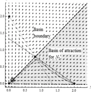
Since there are two possible stable equilibria (i.e. (K,O) or (0,K)) in the "winner-take-all market" above, the initial conditions determine which technology emerges the victor and which ends up the vanquished. To determine which conditions result in which scenario, a phase portrait can be constructed showing the trajectories for the different initial conditions2 . To assist in the sketching of the trajectories, vector fields are drawn to indicate whether the flow is along the N1 axis or N2 axis. The trajectories

for the different initial conditions would be tangent to the vector fields. The set of ini-tial conditions where the trajectory ends in common equilibrium point is called its b a-sin of attraction. Figure 2-2 below plots the trajectories and the baa-sin of attraction for the conditions to a winner-take-all market with N1 as the winner:

Fio r . asi f at A# or (N , 0

I: 4' '4'" 0 '0 PP:.VO e

# (Frank & Cook, 1995)

(Maurer _{& Huberman, 2003)ounda}

20 See Appendix A for details on how to create the phase pfor trait

.0,

(25)

The figure shows two distinct regions (demarcated by the dashed-line) for which initial conditions lead to a different stable equilibrium (N1 or N2). In this situation, the

demarcation (called basin boundary) is a 450 line embodying the similarity of the pa-rameters of the competing technologies. In general, however, this demarcation is a curve owing to the differences in the parameters2 1

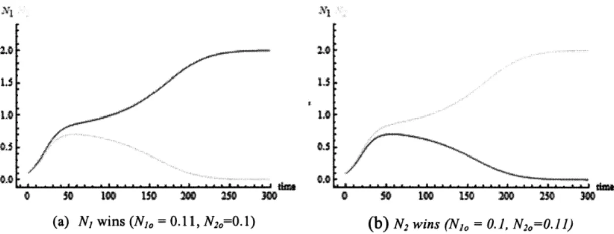
For this case, the better the initial condition is, the better it would fare in the com-petition. This is akin to the maxim that says "whoever has the deeper pocket wins". Examples of the time evolution of N1(t) and N2(t) (red for N1 and green for N2) for

different initial conditions are illustrated in Figure 2-3:

2.0 o 20

1.5 ...

1.0 1. . .

(a) N, wins (N,o = 0.11, N2=0.1) (b) N2 wins (No = 0.1, N2o=0.11) Figure 2-3. Evolution of the competing technologies for different initial conditions

No. and Nz. (Parameter values: rl=r2=O.1, KI=K2 2=2, C12=c21=0.15)

An implication of the model is that the coexistence steady state is independent of the initial conditions. The detailed evolution may differ in time, but the end state would only depend on the carrying capacity and intrinsic growth rate. The initial con-ditions would only matter for winner-take-all scenarios but is not a factor if the tech-nologies are going to coexist. In Chapter 4 we are going to present a model where there are different coexistence steady states and where the system would fall depends on the initial conditions.

(26)

Another implication of the model that is worth capturing is that the steady state values would never be higher than their respective carrying capacity. Figure 2-4 (a) illustrates the time evolution of N1(t) and N2(t) along with the carrying capacity

(dashed line). Note that the values for any time are less than their respective carrying capacity. The coexistence steady state value is also less than its carrying capacity.

This can also be observed by looking at the nullclines for the Lotka-Volterra equa-tions. The nullclines are the curves where either Nl = 0 or N2 = 0 and indicates

whether the flow is along the N1 axis or N2 axis. From Figure 2-4 (b), the nullclines

are lines slanted with negative slopes. Their intersection would provide the steady state value for the coexistence of the two technologies. This intersection would be at

(Nj, N*) which would have values less than their respective carrying capacity (i.e. Nj* < K1,N2* < K2). Later, we will encounter interactions that would result in higher

steady state value than the initial carrying capacity of all or one of the technologies.

3i 0 10 £2 = 2 00 1

L1

13

(a) Time evolution (b) Nullclines

Figure 2-4. Competition coexistence steady state value. (a) Time evolution (b) Phase plane nullclines. (Parameter values: rl=rz=0.1, KI=K2=2, C12=c21=0.05)

(27)

2.2.2 Case 2: Mature and New Technologies

Let us now consider a more general case where the incumbent technology T1 is

al-ready a mature technology with larger carrying capacity K1 = K but slower growth

rate ri = fr .fr is the fraction of the growth rate r2 = r of the incoming new

tech-nology T2. T2 has only a fraction fk of T1's carrying capacity, i.e. K2 = fkK. Let us

again assume that the competitive interaction is symmetric. The results of Table 2-1 reduces to:

Table 2-3. Stability condition for mature technology - new technology competition

Equilibrium Points Stable if

(NI*, N2*) (0,0) Never (K, 0) _c_>_rfk (0, fkK) c > fr fk

rK(fr

-

cfk)

fr2

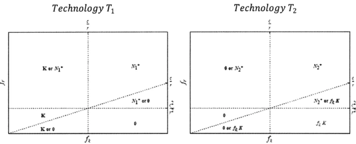
- C2 frrK(fk - c) C < T frr2 - C2

The strategies one can implement would be based on fr and fk. The combinations of these parameters would result in different steady state outcomes. The options and the corresponding pay-off(s) in terms of steady state values are illustrated in Figure 2-5. The N{ and N' shown in the diagram correspond to the non-trivial equilibrium

S rK(frr-cfk) frrK(fk-c)2

fractional intrinsic growth rate fr while decreasing the fractional carrying capacity fk (or increasing its carrying capacity K) would increase its chances of coveting the "winner-take-all" scenario. Conversely, the new entrant technology T2 would benefit

from a smaller fr (or increased growth rate) and a large fk (or increased carrying ca-pacity K2).

(28)

Technology T Technology T2

K 0

Figure 2-5. Strategy options and resulting steady state values for technologies T1 and

T2 based on fractional growth ratef, and carrying capacityfk

As can be seen in the diagrams, there is at least one stable equilibrium, but there are never more than two. If there are two stable equilibria, the initial conditions de-termine into which of the two the system will fall.

An observation however, is that competitive dynamics need not drive competitors out of the market. Examples are available that show established technologies not nec-essarily completely destroyed but surviving - albeit in niche markets or a market dis-tinct from that threatened. The competition between the mainframes and the personal computer did not result in the extinction of the mainframes22_. _{It has been driven}

to-wards a niche market coexisting with the much larger personal computer market. This attribute is something that a new model has to capture.

(29)

(30)

Chapter 3 Lotka-Volterra Interaction

Framework

"If people do not believe that mathematics is simple, it is only because they do not realize how complicated life is."

- John von Neumann

There are different models on the interaction of technologies23 _{and the Lotka-Volterra}

competition model is just but one of them. Implicit however, in the form of the Lotka-Volterra model is a simple framework to define consistently other modes of interac-tions. This chapter covers these modes of interactions and their representative dynam-ics. The results will serve as a reference when we consider the variable competition coefficient in the succeeding chapter.

23 See for instance (Agarwal, Sarkar, & Echambadi, 2002), (Lenox, Rockart, & Lewin, 2007) and the refer-ences cited in there.

(31)

3.1 Classification of Interactions

A classification of the interactions possible can be made based on the effect of the in-teraction on the growth rates of the interacting technologies. Implicit in this frame-work is the positive nature of the coefficients c12 and c21 in the Lotka-Volterra

coupled differential equations. This assumption will be relaxed later when we develop the variable competition coefficient in the succeeding chapter. Within this framework, the effect can be readily discerned by noting the combination of the signs preceding the interaction coefficients c12 and c21 (which were previously confined to competition

interaction), i.e.: N = r1N1 1 _K,-I C2 _K,N1N2 (3.1) ( N2) C21 N₂= 2 N₂ I - NN₂ K2 K₂

For example, pure competition mode would just be one of the interactions possible wherein each technology has negative effect on the other's growth rate. This will be

shown in (3.1) as - c12 and - C21 respectively with C12, C21 > 0. A summary of the

possible modes of interactions is illustrated in Table 3-1:

Table 3-1. Mode of interaction based on the combination of the signs preceding the interaction coefficient

Effect of Ni on Nj's Growth Rate

+cj +

Effect of Nj on N,'s + Symbiosis Predator(Ni) -Prey(Nj)

Growth Rate - Predator(N) - Prey(Ni) Pure Competition

Different dynamics can be obtained from the different modes of interactions24_{. We}

will review these dynamics to provide a reference for the results we are going to ob-tain later.

(32)

3.2 Predator-Prey

3.2.1 Original Predator-Prey

One of the earliest ecological models used in the study of technological evolution were inspired by the works of Volterra2 5. Volterra proposed differential equations for the growth of predators and prey. He assumed that the absence of any prey for susten-ance results in an exponential death rate of the predator. The presence of preys contri-butes to the predator's growth rate by an amount proportional to the available prey as well as to the size of the predator population. Denoting as NJ the population of the predators and N2 that of the prey, this leads to the predator equation:

N1 = - rPN1 + C12N1N2, rl, C1 2 > 0 (3.2)

where rl is the death rate and c12 is a measure on the effect of the presence of the prey

N2 to the predator NI.

For the prey, Volterra considered an unbounded growth in a Malthusian26 way go-verned by its intrinsic growth rate. The presence of predators reduces the growth rate of the prey by an amount proportional to the predator's and prey's population. This leads to the prey equation:

N2 = r2N2 - C2 1N1N2, r2, C2 1 > 0 (3.3)

where r2 is a constant corresponding to the intrinsic growth rate and c21 is measure of

the effect of the predator N1 on the prey N2. The equations were also studied by

Lotka27 in the context of chemical kinetics and hence are called Lotka-Volterra model for predator-prey interactions.

25 (Volterra, 1931)

26 _{(Malthus, 1798)}

(33)

3.2.2 Modified Predator-Prey

The original predator-prey equations as given by (3.2) and (3.3) were a model for predator sharks and prey fishes. This analogy has serious limitations as a long-term model for technological interactions28.For one, the predator is dependent on the exis-tence of the prey. For technology interactions, this is more of an exception than the rule29. What is more prevalent is that technologies exist independent of other compet-ing technologies though their growth may benefit or be inhibited by the interaction with other technologies.

Another limitation is the neutral stability of the results30_{. The results imply an}

os-cillatory interaction where perturbations to the interaction would just move the system to another orbit. This orbit can have larger or smaller amplitude than the original one but in phase with it. If we are going to consider the growth of a technology in terms of the number of units, this would be limited by the number of its eventual users. Data on interaction between technologies have failed to provide an example of long-term oscillations between technologies. It does not have the regularity of the oscillations or the permanence of the interaction.

These limitations are addressed by considering positive intrinsic growth rates but limited by their respective carrying capacities Kland K2. The resulting equations then

become:

(

1 "N C1 2 N1 = r1N1 + -NN 2 (3.4)

(

N2 C2 1 2N N2 = r2N2 -1 2 (

S

K2 I K2

From here on, predator-prey interaction would mean the modified predator-prey inte-raction as given by (3.4). Evident from the form of the coupled differential equations is that the predator technology T1 benefits from the interaction by an amount

28 _{(Samuelson, 1971)}

29 One can cite the case for infrastructure vs. services base competition (Hayashi, 2005). In this case, ser-vice providers use the infrastructure provided by the infrastructure providers while competing with them on the delivery of services.

(34)

C-2NIN₂ . The growth of prey technology T₂on the other hand is inhibited by an K₁

amount - NN 2 .

3.2.3 Critical Dynamics

Given the coupled differential equations in (3.4), we extract the general dynamics for predator-prey interactions. The equilibrium points and stability conditions are tabu-lated in Table 3-2:

Table 3-2. Equilibrium points and stability conditions: Predator-prey interaction

Equilibrium Points Eigenvalues _{Stable if}

(NI*, N2*) (0,0) 11,2 = r, r2 Never (Kj, O) c21K1 c21 > TK2 12 rz _K

K

2 A1 = -r2 (0, K2) C12K2 Never K1 -B + /B2 _{- 4C} r2 (r1K+cl12K2) 1,2 2 Tir2 + C12C2 1 B = r N + r 2 r2 K2 rl(r2K2 - c21K) K K22C2 K Tir2 + C12 C21 = TC 2 +C12C21 NN K K2

From Table 3-2 there are only two stable steady states: the extinction of prey tech-nology T2 or the coexistence of both technologies. Comparison of the predation coef-ficient c21 to the combination of the parameters r2, K2 and K1 determines which

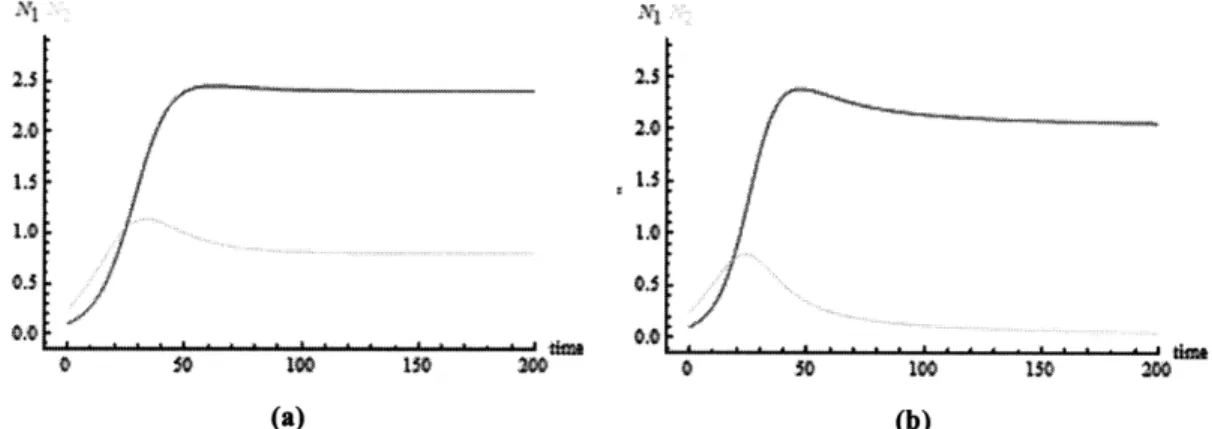
steady state the system would fall into. This result is independent of the initial condi-tions of the technologies.

(35)

Examples of the dynamics are shown in Figure 3-1. The first case (a) depicts the time evolution of the coexistence of both technologies provided that the predation coefficient c21 on T2 is less than _K . The second case (b) illustrates the instance

1

where the predator technology extinguishes the prey technology.

2.0 2.0

0. 0.5

0.0 001 0 go...1 0 00...

$ Mo 0 50 100 ISO 200

(a) (b)

Figure 3-1. Predator-prey sample dynamics: (a) Technologies coexisting; (b) Only

N1 Survives. Parameter values: r1=rz=0.1, KI=K2=2, C12=c21=c

The coexistence steady state for the predator-prey interaction provides a behavior different from the competition model. Compared to the competition model, the nullclines have opposite orientation of the slopes (positive for the red N1 and negative

for the green N2). The intersection of these nullclines is the coexistence steady state

value. Since each nullcline needs to pass through its carrying capacity, the intersec-tion results in a value higher than the carrying capacity for the predator technology (i.e. Nj > K₁) but less than for the prey technology (i.e. N2 < K₂). This is illustrated

in Figure 3-2 where the dashed line correspond to the carrying capacity (in this case

K1 = K2 = 2) which is less than the steady state value of 2.4. This means that the ben-efit to the predator technology in the interaction with the prey technology accrues re-sulting in greater carrying capacity than if there were no interaction present.

(36)

XI = K2 = 2.0 t I" I t "... , .

(a) Time Ion (b) Nullines

(a) Time evolution (b) Nuliclines

Figure 3-2. Predator-prey coexistence steady state value. (a) Time evolution (b) Phase plane nullclines. (Parameter values: r1=r2=0.1, K1=K2=2, C12=C21=0.05)

3.3 Symbiosis

Symbiosis results when both technologies benefit from the relation. This means that the respective growth rates of the interacting technologies are enhanced by the rela-tion. If one looks at the context of mature and emerging technologies, mature technol-ogies are often optimized with regard to its key parameters after a new technology emerges. This "sailing-ship" effect has been observed in different instances and result in the growth of the mature technology31_{. The emerging technology on the other hand,}

may benefit from the infrastructure that was built for the mature technology or from the efforts that have been made to open the market.

The Lotka-Volterra equations for the symbiotic interaction are given by:

N₁_{=iNI(1- )}₁ ₊ _NN ₂

(3.5)

(N 2 C2 1 N2 = r2N2 +

N1

N2

( f K2 K2 31

(37)

3.3.1 Critical Dynamics

The equilibrium points and stability conditions for the coupled differential equations given in (3.5) are tabulated in Table 3-3:

Table 3-3. Equilibrium points and stability conditions: Symbiosis

Equilibrium Points Eigenvalues Stable if

(N*, N2* (0,0) A1,2 = r, r2 Never (K, 0) 2 r2 + _{2 1}K1 Never K₂ /1 = -r 2 (0, K2) c12K2 Never K1 -B + VB2 - 4C r2(Krli+C1 2K2) /1,2 = 2 Ti rr₂- C12C21 _{B = -Nj}1 _{+ -N}r2 rl(K2r2 + C21K) K K2 2 C1 2C2 1 < r1r2 rT2 - C1 2 C2 1 l1r2 - C1 2 C2 1 C = KjK2 )N NN ₂

In the case of symbiosis, there is only one stable equilibrium point. This is achieved when the product of the symbiotic coefficients are less than the product of the intrinsic growth rates. When this condition is not met, the technologies grow without bounds. Examples of symbiotic dynamics are shown in Figure 3-3:

(38)

* so 100

(a)

150d 3 Sim

0 s 1o 15 30

Figure 3-3. Symbiosis sample dynamics: (a) Technologies coexisting (

cz1 2c2 < rzr2); (b) Unbounded growth. Parameter values: r=rzO=0.1, K=K2=2,

C12=C21=c

Whereas only one technology benefits in the predator-prey interaction, symbiosis has both technologies enhanced by their interaction. This is represented by nullclines of positive slopes and an intersection at a point larger than their carrying capacity. This results in non-trivial coexistence values greater than their respective carrying capacity when there is no interaction (i.e. Nj > K1, N2 > K2). This is illustrated in

Figure 3-4:

...

40 10 1 140 l0

(a) Time evolution

Si

. . . s . .. t . . . . i . .

(b ulcie

Figure 3-4. Symbiosis coexistence steady state value. (a) Time evolution (b) Phase plane nulclines. (Parameter values: rl=r2=0.1, KI=K2=2, c12=c2]=0.05)

(39)

3.4 Multi-mode Interaction

A multi-mode model has been proposed where the interaction changes from one mode to another32. This can facilitate description of dynamics where say initially the inte-raction between technologies was initially symbiosis and later turned to pure competi-tion. However, as mentioned early on, there was no mechanism presented to model the transition from one mode to another and the proposal remained descriptive.

This thesis extends the competition model to capture different modes in the com-petition between technologies. Instead of constraining the comcom-petition coefficient to a constant, the coefficient can take on positive or negative values depending on some conditions. The different interaction modes identified in the Lotka-Volterra classifica-tion scheme are incorporated based on the combinaclassifica-tion of the sign of the competiclassifica-tion coefficients c12 and C21 in the competition model, i.e.:

S= rN1 C12 C1 2 ) N(1 N2

(3.6)

2 = 1 N2 C21(N) NN2

where 12 (N2) and C21 (N1) can be positive or negative. The competition coefficient cij (Nj) captures the impact of the competition with N on Ni. By comparing the sign

of the competition coefficient, the Lotka-Volterra interaction classification can be modified in the context of competition as tabulated in Table 3-4:

Table 3-4. Lotka-Volterra classification framework based on the sign of the compe-tition coefficient

Sign of C2 1(N1

)

+

+ Pure Competition Predator(N2) - Prey(N)

Sign of C12(N2)

- Predator(N1)- Prey(N2) Symbiosis

32 _{(Pistorius & Utterback, The Death Knell of Mature Technologies, 1995), (Pistorius & Utterback, A} Lotka-Volterra Model for Multi-mode Technological Interaction: Modeling Competition, Symbiosis, and Predator-Prey Modes, 1996), (Pistorius & Utterback, Multi-mode Interaction among Technologies, 1997)

(40)

In the following chapter, we will provide a mechanism that would enable the switching from one mode to another. Specifically, it presents a form of the competi-tion coefficient that can switch from positive to negative values and vice versa de-pending on the size of the variable N. We believe this is the first instance to imple-ment the Lotka-Volterra multi-mode framework within the context of technology inte-raction.

(41)

(42)

Chapter 4 Variable Competition Coefficient

"The only constant is change." Heraclitus

Whereas the previous chapter showed dynamics exclusive to a particular mode of in-teraction, this chapter presents a Lotka-Volterra competition model with variable competition coefficient that integrates the different dynamics. It uses the concept of cost and benefit to model the variation of the competition coefficient. It then utilized the results of the previous chapter to dissect the different modes of interaction possi-ble in the evolution of the competition.

4.1 Variation in the competition

The assumption of a constant coefficient clearly simplifies the dynamics of competi-tion between technologies. We posit that in reality, the competicompeti-tion between technolo-gies changes from one mode to another depending on several drivers. These drivers may include the elaborate strategy to enter a market segment, the constraints within a technology, or the influence of regulation to enforce a particular interaction.

Broadly, what we are after is a competition that can exhibit variations in the inte-raction. For simplicity, we can consider the competition between an incumbent

(43)

tech-nology and an emerging new techtech-nology. We contend that when an emerging technol-ogy has a small size33, the interaction with an incumbent technology is generally symbiotic. However, as the emerging technology grows the interaction eventually shifts to a more intense competition. A possible sketch of the behavior of the competi-tion coefficient is illustrated in Figure 4-1:

COOPERA ~-\E

Figure 4-1. Varying competition coefficient (solid line) and constant coefficient (dashed line)

It is no coincidence that the profile we have sketched is similar to a company life cycle. The characteristic growth patterns of companies correspond to patterns of cash generation and usage. However, instead of using time as the independent variable, we take the size of the technology as the proxy. This has the added benefit of dynamically moving "forward" and 'backward" whereas time can only move forward. We are going to exhaust the analogy to these patterns when we weave the mathematical form of the competition coefficient from the benefits the competition provides and the costs it entails.

33 _{We liberally use "size" to mean any of the pertinent variables describing the evolution of the technology,}

(44)

4.1.1 Cooperative Competition

Figure 4-1 illustrates a case where initially the competition is cooperative but as the size Nj of technology Tj increases, the competition switches to destructive competi-tion. When the competition coefficient is negative, it shows up as a positive interac-tion term in the Lotka-Volterra equainterac-tion. This provides a "cooperative" effect where the relation enhances the growth rate of the particular technology. Cooperative com-petition may manifest when technologies work together for part of technology devel-opment or access to marketplace. The concept has become popular and the new term "co-opetion" has been coined to describe it34

The degree to which the market was expanded by an innovative technology is a factor that affects the variation of the competition. It has been shown that disruptive technologies that expand markets will almost always come from outside the indus-try3 5. In industries where the market is not yet well established, symbiosis is often the initial dominant interaction between technologies. When the market becomes well es-tablished, symbiosis decreases and the companies aligned to a particular technology become more competitive36

It is not uncommon for one proponent of a technology to be initially "cooperative" to another company whose technology may be a competitor if in doing so provides more benefit to it. An example that comes to mind is the relationship of Yahoo! and Google with regards to search technologies. Yahoo was an early investor of Google and used Google's search engine before it bought Inktomi and competed head-on with Google3 7. Many traditional pharmaceutical companies collaborate with new entrants to adapt the technology and build their competencies. The license of Humulin, a hu-man insulin based on recombinant DNA, by Genentech to Eli Lily is an example of this38

34 _{(Brandenburger & Nalebuff, 1996)}

35 (Utterback, Mastering the Dynamics of Innovation, 1994) 36 _{(Tisdell, 2004)}

37 (Iyer, Lee, & Venkatraman, 2006). An aside, though they have been fierce competitors since then, there are rounds of talks for possible partnership in search advertising.

(45)

4.1.2 Destructive Competition

On the other hand, when the competition coefficient is positive, the impact is destruc-tive - it inhibits the growth of the technology. Within the Lotka-Volterra classification scheme, the technology may be the prey in predator-prey interaction or one of the competitors in the pure competition mode. Either scenario inhibits the growth of the technology.

It was mentioned earlier the possibility of a lower performing (in the traditional metric) technology to attack from below before competing head-on with the estab-lished technology in the mainstream market39. Such approach is not limited to an "at-tack from below" (lower performance, lower cost, higher ancillary benefits) but other combinations have resulted in one technology eroding the share of the other technolo-gy40. The substitution of the vinyl album by the compact disc technology (higher per-formance, lower cost, higher ancillary benefits), film camera by digital cameras (low-er p(low-erformance, high(low-er cost, high(low-er ancillary benefits) and the slide rule by the elec-tronic calculator (higher performance, higher cost, lower ancillary benefits) are just but a few of the examples. Taken together, these examples provide a picture of an in-cumbent technology providing a new entrant with a market to grow and later preyed by it in the mainstream market.

Destructive competition does not necessarily end in the complete destruction of the technology. As long as the intrinsic growth rate is higher than its competition rate, the technology will survive. What the previous competition model predicts, however, is that the coexistence of both technologies would always result in a steady state value less than their respective initial carrying capacities. We have shown earlier that in a predator-prey interaction, there would be an "increase" in the carrying capacity of the predator technology accrued from the interaction with the prey technology. The varia-ble competition coefficient reflects this behavior.

39 (Christensen, Innovator's Dilemma: When New Technologies Cause Great Firms to Fail, 1997)

(46)

4.2 Form of the Competition Coefficient

An earlier section has alluded to the company life cycle as a pattern for the competi-tion coefficient. A specific form of the competicompeti-tion coefficient can be obtained base on the cost it entails to compete and the benefits or rewards the competition would bring about. There might be different factors to consider for the cost and benefit but for our purpose we consider the case where the cost and benefit varies depending on the size N of the competing technologies. As in the earlier models, this size attribute can be the number of units sold or the extent of its market share. The analysis follows similar treatment in ecology where shifts from beneficial to detrimental roles in the association between species have been observed based on their population density41

4.2.1 Benefit Function

For purposes of illustration, let us consider an emerging market. In the early stage of an emerging market, the perceived opportunity is large. No technology is dominant and there is substantial uncertainty in the market as well as in the technology. During this fluid phase, the rate of experimentation and innovation grows42. For the compet-ing technologies there is not that much benefit for an intense competition at this early stage. As the uncertainty on the technology and market potential are resolved, the stakes become higher and the benefits clearer. This benefit grows as its size increases reaching a threshold value where all the addressable market of technology T have been captured. A function that would have these attributes is:

a N2

Benefit for T competing with T = + 2 (4.1)

The coefficients ai and yi are properties of T that modulate the impact of competition

with Tj. ai is the maximum extent of the benefit Tj can derive in competing with Ti

while yidictates the value of N where the rate of increase of the benefits are

increas-41 _{(Hernandez, Dynamics of Transitions between Population Interactions: A Nonlinear Interaction} alpha-Function Defined, 1998), (Hernandez & Barradas, Variation in the Outcome of Population Interactions: Bifurcations and Catastrophes, 2003)

(47)

ing the fastest (at i). The behavior of the benefit function and its associated parame-ters are illustrated in Figure 4-2:

Cit

V

x.1

Figure 4-2. Benefit function and associated parameters

Increasing the value of ai results in higher loss to Ti in the interaction with T7. This

redounds to a higher benefit for T. Increasing yi on the other hand delays the full im-pact of the competition at larger value of N.

4.2.2 Cost Function

In conjunction with the benefits, the competing technologies bear the costs of compe-tition for a share in the market. Substantial risks are borne by the companies to ex-plore the technology, develop the market and compete with other players. Relative to the initial size of the technology, the cost of competition is high at its nascent stage. This cost reaches a maximum when the size of the technology is yi. The cost then de-clines as the technology increases its traction with the market. Similar observation has been made where the advantage of size relates to greater market power and efficient

scale43. These attributes can be modeled by the function:

(48)

fli N

Cost for Tj competing with i =2

Yj + N' (4.2)

Similar to the benefit function, the coefficients fli and yjare properties of technology Ti related to competition with technology Tj. fli is proportional to the maximum cost it

would entail to compete with T in the market. yi on the other hand specifies the size

Nj where that cost is maximum. The behavior of the cost function and its associated

parameters are illustrated in Figure 4-3:

kxe .~"

ta ,i

Figure 4-3. Cost function and associated parameters

The larger fli is, the higher the cost impact to Tj the competition would T entails. In-creasing yi would lessen the impact and at the same time delay to higher value of N.

4.2.3 Variable Competition Coefficient

The competition coefficient will be defined as the difference of the benefit and the cost function. The competition would be cooperative as long as the cost to "aggres-sively" compete is much higher than the benefit it provides. The competition coeffi-cient would then take the form:

(49)

ci = Benefit for Tj competing with Ti

- Cost for Tj competing with Ti

yThe behavior of the resulting competition coefficient is given in Figure 4-4: The behavior of the resulting competition coefficient is given in Figure 4-4:

(4.3) beasfit 11 W NIV 2 cost .. ,*c~:* -- Ii -aw~', N.': ,al 3-1

Figure 4-4. Variable competition coefficient

As can be seen from Figure 4-4, the competition coefficient would be equal to the constant c; = ai as N -+ oo or as N grows very large. For N less than -, the impact

a1

of the competition is cooperative. For T the cost of competing with T outweigh the benefits and hence is cooperative to it. Beyond , _{however, the attitude of T shifts to}

destructive knowing that more benefits can be obtained in the competition with Ti. Using the form of the competition coefficient, the Lotka-Volterra competition eq-uations then take the form: