HAL Id: insu-02115602
https://hal-insu.archives-ouvertes.fr/insu-02115602
Submitted on 30 Apr 2019HAL is a multi-disciplinary open access archive for the deposit and dissemination of sci-entific research documents, whether they are pub-lished or not. The documents may come from teaching and research institutions in France or abroad, or from public or private research centers.
L’archive ouverte pluridisciplinaire HAL, est destinée au dépôt et à la diffusion de documents scientifiques de niveau recherche, publiés ou non, émanant des établissements d’enseignement et de recherche français ou étrangers, des laboratoires publics ou privés.
Optimal Estimation Method (OEM)
Ghazal Farhani, R. Sica, Sophie Godin-Beekmann, Alexander Haefele
To cite this version:
Ghazal Farhani, R. Sica, Sophie Godin-Beekmann, Alexander Haefele. Stratospheric Ozone Density Retrieval Using the Optimal Estimation Method (OEM). EPJ Web of Conferences, EDP Sciences, 2018, 176, pp.art. 03006. �10.1051/epjconf/201817603006�. �insu-02115602�
STRATOSPHERIC OZONE DENSITY RETRIEVAL USING THE
OPTIMAL ESTIMATION METHOD (OEM)
Ghazal Farhani1,*, R. J. Sica1, Sophie Godin-Beekmann2,1and Alexander Haefele3,1
1Department of Physics and Astronomy, The University of Western Ontario, Canada ∗[email protected]
2Université de Versailles Saint-Quentin en Yvelines, France 3Federal Office of Meteorology and Climatology MeteoSwiss, Switzerland
ABSTRACT
We use an Optimal Estimation Method (OEM) to retrieve ozone profiles from the CANDAC Stratospheric Ozone Differential Absorption Lidar in Eureka, Canada. The OEM is a well known inverse method in which a forward model (FM) is used to describe the instrument and geophysical situation. We have developed a FM and are testing its validity using synthetic measurements. We will present the advantages of using OEM retrievals over the traditional method, including a full uncertainty budget.
1 INTRODUCTION
Ozone is a minor constituent in the atmosphere but plays an important role by absorbing harm-ful ultraviolet (UV) radiation emitted by the Sun. The bulk of the protective ozone re-sides in the stratosphere (an altitude range of about 12 to 50 km) while a small but signif-icant amount exists near the surface, where it is pollutant. Significant chemical depletion of the ozone during late winter and spring has been observed over both Poles [1]. Ozone holes are linked to the emission of chlorine and bromine compounds (the so-called Ozone De-pleting Substances or ODS). Since the Montreal Protocol came to effect, the emission of ODSs has been decreased. In order to evaluate the re-covery of ozone as a result of this change, con-tinuous measurements of stratospheric ozone is required. Measurements of stratospheric ozone have been carried out using the Differential Ab-sorption Laser technique Lidar (DIAL) in
Eu-reka, Nunavut at the Polar Environment Atmo-spheric Research Laboratory (79.98° N, 85.94° W, 647 m above sea level) for more than 20 years. In the DIAL method, two different laser wavelengths are simultaneously transmitted to the atmosphere. One wavelength is in a spec-tral region with a high absorption by ozone (for stratospheric measurements typically 308 nm) and is called the "on-line" wavelength. The other wavelength has a low absorption by the ozone (typically 353 nm) and is called the "off-line" wavelength.
2 Algorithms to Retrieve Ozone Density for the DIAL System
The lidar equation gives the intensity of the backscattered photons for a monochromatic laser pulse at wavelength λ , in an atmospheric layer located at altitude z, and acquired during an integration time ∆t: N(z,λi) = N0(λi)η(λi) A z2β (λi,z) × exp[−2 z 0 α(z′,λi)dz ′] (1)
where N0(λi) is the emitted number of photons,
η(λi) is the optical efficiency of the
receiv-ing system, A is the telescope area, β (z,λi) is
the atmospheric backscattering coefficient and α(z,λi) is the atmospheric extinction coefficient
and ozone profiles can retrieved as follows: no3(z) = −1 2∆δo3(z) d dzln N(λ1,z) − Nb1 N(λ2,z) − Nb2 + δ no3(z) (2)
where N(λ1, z) and N(λ2, z) are, respectively,
the on-line and off-line signals at altitude z, Nb2
and Nb2 are corresponding background signals,
∆δo3(z) = δo3(λ1) − δo3(λ2) is the differential
absorption cross section, and δ no3(z) is a
cor-rection term. The detailed calculation is pre-sented in [3] and [4].
The Optimal Estimation Method (OEM) is a well known method in the passive remote sens-ing method; however, it has only been recently used to retrieve atmospheric quantities with li-dar measurements (for example [5]). The OEM has many advantages such as providing a full uncertainty budget, including both systematic and statistics errors of the retrieved profiles. In the OEM method, (unlike the traditional method) no pre- or post- filtering of retrievals is required (often digital filters will introduce uncertainties to the final result [3]). Moreover, the sky background correction can be retrieved along wihh the ozone density profile. A brief introduction of the method is covered in the next section. Comprehensive details on the sub-ject can be found in [6].
3 METHODOLOGY
The Optimal Estimation Method (OEM) is a matrix inverse method based on Bayes′ theo-rem. Let x= (x1,x2, ...,xn) be the state vector of the atmosphere and y= (y1,y2, ...,yn) be the corresponding measurement vector. The rela-tionship between x and y is called the forward model (FM):
y= F(x,b) + ε (3)
where b is the model parameter vector andε is the measurement error vector. For non linear
problems, the FM can be linearized: y− F(xa) =
∂ F
∂ y|xa(x − xa)
+O(x2) ≈ K(x − xa)
(4)
where Kx= ∂ F∂ y is the Jacobian matrix and
rep-resents the sensitivity of the observation vari-ables y to the state varivari-ables x [6]. The K represents a linearization of the forward model around x. It initially needs to be calculated for the a priori xa, and then recalculated for the
updated values of x during the iterative conver-gences to the solution. The iteration continues to minimize the cost function J(x):
J(X) = [y − F( x,b)]TS−1y [y − F( x,b)] +[x − x]TS−1a [x − x]. (5) The solution is:
x= xa+ SaKT(KSaKT+ Sa)−1(y − Kxa) (6)
where Saand Sεare the uncertainties associated
with an a priori state and measurements, their diagonal elements are the variances of the indi-vidual elements of the a priori state and mea-surements error.
3.1 Applying the OEM for Ozone Profile
Retrieval
Using two uncorrelated measurements we are producing first ozone retrievals. For the pi-lot study, we are testing the OEM on synthetic measurements. After being confident about the results, we will apply our method to real mea-surements. Determining the appropriate FM is one of the main challenges in the OEM. We are using the lidar equation as our FM.
N(z,λi) = N0(λi)η(λi) A z2β (λi,z) ×exp[−2 z 0 α(z′,λi)dz′] + B. (7)
Here, N(z,λi) represents the detected photons
(without applying any correction). In the DIAL method two wavelengths are simultaneously
Figure 1: Synthetic countrate for 3 hours of DIAL measurements on Feb. 28, 2016. Left panel: high channel (blue curve, real measurements; red curve, synthetic measurements). Right panel: low channel.
transmitted. We only use the on-line wave-length for our calculations for this initial study, but are currently extending the retrieval to use both data channels.
4 RESULTS
Using the US standard atmospheric model ozone profile we made our synthetic measure-ments for both high and low Rayleigh channels at 308 nm (see Figure 1). These profiles are similar to 3 hours of the Eureka DIAL measure-ments on 28 of February 2016. We assumed a constant background in generating our syn-thetic measurements. The assumption provides a good fit for the low channel counts. How-ever, the background count for the high chan-nel above 60 km due to the signal induced noise (SIN) effect is not a constant value. We plan to include the effect of SIN offset on the back-ground counts in the near future.
We used the same ozone profile for our a pri-ori, therefore, we expect to get the optimal so-lution without any iteration. The averaging ker-nel shows the sensitivity of the retrieval to the vector state. As shown in Figure 2, the averag-ing kernel equals 1 below 40 km which means the retrieved profile below this altitude is
inde-pendent of the a priori information. The sen-sitivity of the averaging kernel decreases with increasing altitude.
Figure 2: Averaging kernel for the ozone profile for the measurements shown in Fig.1. The averaging kernel equals 1 below 40 km.
The residuals (see Figure 3) show the difference between the FM and the measurements (here the synthetic data). The residuals (shown in blue) are within the FM uncertainty (shown in red).
Figure 3: Residuals between the forward model and the measurements for the low and high channels (blue). The red lines show the standard deviation of the measurements.
Figure 4 shows the retrieved ozone profile. The retrieval grid is extended from 7 km to 50 km. The retrieved ozone profile tends to fall back
to the a priori ozone profile at altitudes above 40 km which is predictable as the sensitivity of the averaging kernel is decreasing above this height. The cost of this retrieval is 1.03.
Figure 4: Retrieved ozone profile (red curve) using the OEM.The blue curve is the a priori ozone profile used by the OEM.
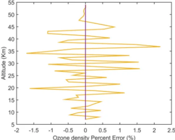
The difference between the retrieved profile and the a priori profile is shown in Figure 5.
Figure 5: The percentage error between the re-trieved ozone profile and the a priori ozone profile.
5 CONCLUSIONS
We use an Optimal Estimation Method (OEM) to retrieve ozone profiles from synthetic mea-surements from 7 km to 50 km. The retrieval
is currently being extended to include back-ground counts and the lidar constants using two data channels. We are also planning to retrieve the aerosol extinction coefficient. We also are analysing real measurements and are validating the retrievals against other measurements.
ACKNOWLEDGEMENTS
We thank the Natural Science and Engineer-ing Research Council (NSERC), the Canadian Space Agency (CSA) and, the Northern Scien-tific Training Program (NSTP).
References
[1] S. Solomon. Stratospheric ozone depletion: A review of concepts and history. Reviews of Geo-physics, 37(3):275–316, 1999.
[2] R. M. Measures. Laser Remote Sensing: Fun-damentals and Applications. Krieger Pub Co; New edition edition (August 1991).
[3] S. Godin, A. Carswell, D .Donovan, H. Claude, W. Steinbrecht, S. McDermid, T. McGee, M. Gross, H. Nakane, D. Swart, et al. Ozone differential absorption lidar algorithm inter-comparison. Applied optics, 38(30):6225– 6236, 1999.
[4] T. Leblanc and F. Gabarrot. Critical assessment and standardized reporting of vertical filtering and error propagation in the data processing al-gorithms of the ndacc lidars. Technical report, NDAAC, 2015.
[5] R. J. Sica and A. Haefele. Retrieval of temper-ature from a multiple-channel rayleigh-scatter lidar using an optimal estimation method. vol-ume 54, pages 1872–1889. OSA, Mar 2015. [6] C. D. Rodgers. Inverse Methods for
Atmo-spheric Sounding: Theory and Practice. World Scientific Publishing, 2000.