HAL Id: hal-00501631
https://hal.archives-ouvertes.fr/hal-00501631
Submitted on 10 Jun 2015
HAL is a multi-disciplinary open access
archive for the deposit and dissemination of
sci-entific research documents, whether they are
pub-lished or not. The documents may come from
teaching and research institutions in France or
abroad, or from public or private research centers.
L’archive ouverte pluridisciplinaire HAL, est
destinée au dépôt et à la diffusion de documents
scientifiques de niveau recherche, publiés ou non,
émanant des établissements d’enseignement et de
recherche français ou étrangers, des laboratoires
publics ou privés.
for very short-lived halogenated species
Ignacio Pisso, P. H. Haynes, Kathy S. Law
To cite this version:
Ignacio Pisso, P. H. Haynes, Kathy S. Law. Emission location dependent ozone depletion potentials
for very short-lived halogenated species. Atmospheric Chemistry and Physics, European Geosciences
Union, 2010, 10 (24), pp.12025-12036. �10.5194/acp-10-12025-2010�. �hal-00501631�
www.atmos-chem-phys.net/10/12025/2010/ doi:10.5194/acp-10-12025-2010
© Author(s) 2010. CC Attribution 3.0 License.
Chemistry
and Physics
Emission location dependent ozone depletion potentials for very
short-lived halogenated species
I. Pisso1,2,*, P. H. Haynes1, and K. S. Law2
1DAMTP, University of Cambridge, Cambridge, UK
2UPMC Univ. Paris 06; Universit´e Versailles St-Quentin en Yvelines; CNRS/INSU; LATMOS/IPSL, UMR 8190,
Paris, France
*now at: Research Institute for Global Change, JAMSTEC, Yokohama, Japan
Received: 20 May 2010 – Published in Atmos. Chem. Phys. Discuss.: 30 June 2010
Revised: 16 November 2010 – Accepted: 20 November 2010 – Published: 17 December 2010
Abstract. We present trajectory-based estimates of Ozone
Depletion Potentials (ODPs) for very short-lived halogenated source gases as a function of surface emission location. The ODPs are determined by the fraction of source gas and its degradation products which reach the stratosphere, depend-ing primarily on tropospheric transport and chemistry, and the effect of the resulting reactive halogen in the stratosphere, which is determined by stratospheric transport and chem-istry, in particular by stratospheric residence time. Reflect-ing the different timescales and physico-chemical processes in the troposphere and stratosphere, the estimates are based on calculation of separate ensembles of trajectories for the troposphere and stratosphere. A methodology is described by which information from the two ensembles can be com-bined to give the ODPs.
The ODP estimates for a species with a fixed 20 d life-time, representing a compound like n-propyl bromide, are presented as an example. The estimated ODPs show strong geographical and seasonal variation, particularly within the tropics. The values of the ODPs are sensitive to the inclu-sion of a convective parametrization in the trajectory cal-culations, but the relative spatial and seasonal variation is not. The results imply that ODPs are largest for emissions from south and south-east Asia during Northern Hemisphere summer and from the western Pacific during Northern Hemi-sphere winter. Large ODPs are also estimated for emissions throughout the tropics with non-negligible values also ex-tending into northern mid-latitudes, particularly in the sum-mer. These first estimates, whilst made under some simpli-fying assumptions, show larger ODPs for certain emission
Correspondence to: I. Pisso
regions, particularly south Asia in NH summer, than have typically been reported by previous studies which used emis-sions distributed evenly over land surfaces.
1 Introduction
It is now well established that long-lived halocarbons (e.g. CFCs, HCFCs, solvents etc.) have contributed to the de-struction of ozone in the stratosphere over at least the last 30 years (WMO, 2007). The impact of halogen containing substances on stratospheric ozone depletion has been quan-tified using Ozone Depletion Potentials (ODPs), which are defined as the time-integrated ozone depletion resulting from unit mass emission of that substance relative to that resulting from a corresponding unit mass emission of CFC-11 (CCl3F)
(Wuebbles, 1983; Solomon et al., 1992; WMO, 2007). ODPs are most easily defined for substances with long atmospheric lifetimes (greater than about 6 months). For these substances, which are well mixed in the troposphere, the ODP is indepen-dent of the emission time and location.
There is now increasing interest in stratospheric ozone de-pletion due to halogen-containing substances with lifetimes of 6 months or less, now conventionally called Very Short-lived Substances (VSLS). These are currently estimated to make a small contribution to the stratospheric chlorine load-ing (WMO, 2007) but a significant contribution to total stratospheric bromine, Bry. This contribution has been
in-ferred from stratospheric BrO data, independent estimates from upper tropospheric measurements of VSLS and mod-eling studies (e.g. Dorf et al., 2008; Kerkweg et al., 2008a,b; Aschmann et al., 2009; Hossaini et al., 2010) and is estimated to be 3 to 8 ppt bromine out of a total Bryloading of 18 to
25 ppt (WMO, 2007). Given that anthropogenic emissions of long-lived brominated halons and methyl bromide appear to be decreasing, the relative contribution of brominated VSLS to total stratospheric bromine, and hence to ozone depleting reactive bromine, is likely to increase in the future. Within the stratosphere reactive bromine destroys ozone more effec-tively, by a factor of 60, than reactive chlorine on an atom-by-atom basis (WMO, 2007). Reactive iodine species would destroy ozone even more effectively but are considered to be less important given current knowledge of emissions and hence of likely stratospheric iodine loading.
At the present time, VSLS emissions are dominated by natural emissions with only 5% or less coming from human sources although these may increase in the future. For exam-ple, n-propyl bromide, (nC3H7Br, hereafter n-PB) is a
non-natural VSLS already used as a fumigant and proposed as a solvent replacement. Other VSLS have also been pro-posed such as iodotrifluoromethane (CF3I) for use as a halon
replacement and phosphoroustribromide (PBr3) for in-flight
aircraft engine fire suppression. Furthermore emissions of natural halogenated VSLS may increase as a result of cli-mate change, e.g. from oceans in response to increasing sea surface temperatures (e.g. Butler et al., 2007).
VSLS are not well-mixed in the troposphere and there-fore estimation of their ODPs needs to take into account the details of the spatial distribution of emissions. This point has been recognized for some time (Solomon and Albritton, 1992) but to date only a limited number of quantitative es-timates exist (e.g. Wuebbles et al., 2001, 2009) since such estimates require the use of global models including both tro-pospheric and stratospheric processes. For each ODP assess-ment several model integrations are required at significant computational cost and due to large uncertainties in the spa-tial and temporal distributions of VSLS emissions, different emission scenarios also need to be evaluated.
A methodology is required which provides VSLS ODPs as a function of surface emission location directly. Here, we present such a methodology based on a trajectory mod-elling approach. The advantage of using trajectories is that transport characteristics from particular locations and their impact on ODPs can be clearly identified without the need to perform multiple integrations as in the case of ODP evalua-tion using global Eulerian models. The ODP depends on the fraction of VSLS, or more precisely the fraction of the total emitted halogen, emitted from a given location reaching the stratosphere and the residence time in the stratosphere, dur-ing which ozone depletion can occur due to the reactive halo-gen arising from the emission. Ensembles of tropospheric trajectories including a representation of total halogen degra-dation are used to quantify the fraction reaching the strato-sphere. Stratospheric trajectories, run for longer time peri-ods, are used to quantify stratospheric residence time. The information from the two sets of trajectories is combined to estimate the VSLS ODP as a function of emission location.
A major goal of this paper is to present the methodology (Sect. 2) and in this first step simplifying assumptions have been made with regard to VSLS processing, loss and impact on ozone. However, we believe that the conclusions are ro-bust to relaxing these assumptions. ODPs are presented in Sect. 3 for a VSLS with a 20 d lifetime, representing a com-pound like n-PB, and compared to previous studies. Conclu-sions are given in Sect. 4.
2 Methodology
The processes controlling VSLS ODPs have been set out in WMO (2003, Chapter 2). As for long-lived species, any halogen-containing source gas (SG) emitted at the surface is exported into the free troposphere and thence potentially transported into the stratosphere. For VSLS in particular, a significant fraction of the SG is expected to degrade pho-tochemically during the transit to the stratosphere, produc-ing halogen-containproduc-ing product gases (PG). The PG may themselves degrade photochemically, or since many are sol-uble, may be removed by rainout or by other cloud processes (WMO, 2007). The total halogen reaching the stratosphere potentially includes contributions from SG and PG.
Motivated by the above, the semi-empirical estimate for the ODP of a long-lived species was extended in WMO (2003) to a VSLS, X, to be: ODPX(xe,te) = (rXSG(xe,te)ζXSG+rXPG(xe,te)ζXPG) ·αnBr+nCl 3 · TXactive(xe,te) TCFCactive-11 ·MCFC-11 MX (1)
where xe and te are, respectively the location and time of
emission. This is essentially the form given in (2.14) of WMO (2003) presented in a notation that is more compat-ible with that for a long-lived species presented in WMO (2007). Here rXSG(xe,te)and rXPG(xe,te)respectively are the
mass fractions of the source and product gases that reach the stratosphere (measured relative to the mass of the emitted source gas). TXactive(xe,te) is the time spent in the
strato-sphere by the active halogen that results from the breakdown of X (and correspondingly for TCFCactive-11). Note that the pos-sible dependence on xe and te is retained in TXactive(xe,te).
WMO (2003) refer to TXactive(xe,te)as a stratospheric
resi-dence time, which can be justified on the basis that the active species that result from breakdown of X are soluble or have short tropospheric lifetimes, so that once the active species leaves the stratosphere and enters the troposphere it will be removed. nBr and nCl are respectively the number of the
bromine and chlorine atoms in one molecule of X and α is an “efficiency factor” for ozone destruction by reactive bromine relative to that by reactive chlorine. The efficiency factors ζXSGand ζXPG are included since the ozone depletion result-ing from the halogen released by breakdown of source gases or product gases will not depend only on the residence time
TXactive(xe,te)but also on details of where exactly the
halo-gen is released and on its subsequent path through the strato-sphere. For the remainder of this paper ζXSG and ζXPG are both taken to be equal to 1 (but they could be estimated more precisely from a suitable model calculation). These factors should also arguably depend on xeand tebut this dependence
has been ignored as a first approximation. Mass fractions are converted into molar fractions by the quotientMCFC−11M
X of molecular masses of CFC−11 and X. Note that the Eq. (1) holds not only for VSLS, but also for a long-lived species, for which rSG=1 and rPG=0. The Eq. (1) highlights that in estimating ODPs for VSLS there are two major and somewhat independent considerations. The first is the path taken through the troposphere, which determines rXSG(xe,te)
and rXPG(xe,te), and the second is the path taken through the
stratosphere, which determines TXactive(xe,te). Given
knowl-edge of ODPX(xe,te), the ODP for an arbitrary emission
dis-tribution in location and time can be calculated by a weighted integral of ODPX(xe,te).
The processes removing SG and PG are distinct, and for detailed calculations of ozone depletion the partitioning of halogen reaching the stratosphere between SG and PG may be important (WMO, 2007). However, in a first-order de-scription, what is important is the total halogen reaching the stratosphere. In the following development of a method for calculating ODPs for VSLS we shall, for simplicity, assume that it is sufficient to consider total halogen, i.e. to regard X as a family that includes the SG and all the resulting halogen-containing PG and degradation products, but it would be straightforward to extend the method and relax this assump-tion.
Consider now the depletion of ozone in the stratosphere, recalling that ODPs are fundamentally a linear concept that quantifies the effect of a unit emission on a given background atmosphere. Therefore, during its passage across the strato-sphere, X can be taken to destroy ozone, measured by mass concentration, at a local rate which is proportional to the lo-cal mass concentration of X, with a constant of proportion-ality equal to KX, so that KX has units of inverse time. KX
encodes information not only on the reactivity, but also on the fraction of X (recall that X is now being regarded as a chemi-cal family) that appears in active form together with the back-ground concentrations of ozone and other species that influ-ence the rate of destruction.
The time integrated depletion of ozone in a region of the stratosphere due to a unit mass emission of X released at location xe and time te in the troposphere can therefore be
written as: 1O3(X,xe,te)= Z ∞ te Z ρX(x,t,xe,te)KX(x,t )dxdt (2)
The integration variables x and t represent positions and times in the stratosphere. ρX(x,t,xe,te)is the density of X
(total halogen) at position x and time t resulting from the pulse emission of X at position xeand time te.
Evaluation of the integral in Eq. (2) requires prediction of the density ρX(x,t,xe,te)through solution of the equations
for transport and chemical reaction given the pulse emis-sion at xe,te. This prediction could be based on an
Eule-rian chemical transport model, but here we follow chemical evolution along trajectories using a Lagrangian approach. In other words we assume that:
ρX(x,t,xe,te) = hrX(t ;X)δ(x − X(t;xe,te))i (3)
where x=X(t;xe,te)describes, as t varies, a trajectory
be-ginning at position xeat time te. δ() is the Dirac delta
func-tion. rX(t ;X) is a number between 0 and 1 representing
the variation of total amount of halogen species X, so that rX(te;xe) =1, with rX(t ;X(t;xe,te))expected to decay as t
increases from te. The brackets hi denote an average over
a suitable ensemble of trajectories emitted at xe,te carrying
initially a unit mass of the species X in SG form. This av-eraging could, for example, reflect the fact that variation of 1O3(X,xe,te)with respect to xeor te is necessarily
coarse-grained – i.e. an ensemble of trajectories with launch position close to xeor launch time close to teis considered and an
av-erage is taken over that ensemble, or it could be that some kind of stochastic parametrization is required in following the trajectory X(t;xe,te), e.g. many realisations of a random
walk representing diffusion (e.g. Legras et al., 2003) or in-deed convective effects, followed by an average over an en-semble of such realisations.
We may substitute Eq. (3) into Eq. (2), to give
1O3(X,xe,te) = h Z ∞ te dt Z dx rX(t ;X)δ(x − X(t ;xe,te))KX(x,t)i = h Z ∞ tin(,X) dt rX(t ;X)KX(X(t;xe,te),t )i (4)
where tin(,X) is the time at which the trajectory X first
en-ters the stratosphere. tout(,X) may be defined
correspond-ingly as the time the trajectory first leaves the stratosphere. Note that if followed long enough the trajectory X will enter and leave the stratosphere many times. However the active part of the halogen will, to good approximation, leave only once since, once it re-enters the troposphere it will be rapidly lost due to rainout.
We can instead write KX=χXactiveKXactive where χXactiveis
the proportion of X appearing in the active form and then regard χXactivenot as representing the active part of X aris-ing in a saris-ingle circuit of the trajectory through the strato-sphere, but as a sum of the parts arising in all such circuits. The active fraction χXactivecorresponds to the factors ζSGand ζPGin Eq. (1). The integral appearing in Eq. (4) is then not taken over the entire trajectory subsequent to first entry into the stratosphere, but instead only over the part of the trajec-tory corresponding to first passage through the stratosphere, i.e. the upper limit of the integral is taken to be tout(,X)
all circuits applies only to a long-lived species, since it might reasonably be assumed that for VSLS the conversion to the active form during one circuit is complete, but the generali-sation is useful since the resulting formalism then applies to all halogenated substances, regardless of lifetime.
This alternative formulation allows rX(t ;X) to be
consid-ered constant for t >tin(,X). The subsequent loss of
to-tal halogen is incorporated by the definition of χXactiveas the cumulative distribution function for conversion to the active species, regarded as function of position and then sampled by the trajectory. The change of the upper limit to the integral allows Eq. (4) to be re-expressed as:
1O3(X,xe,te)=hrX(tin();X)
Z tout(,X)
tin(,X)
dt χXactive(X(t;xe,te))KXactive(X(t;xe,te))i (5)
where the factor rX(tin(),X) in Eq. (5) is determined
by the tropospheric trajectory segments and the integral is determined by the stratospheric trajectories. For VSLS, rX(tin(),X) is expected to be significantly less than one,
since total halogen, in both SG and PG, reaching the strato-sphere is expected to be only a small fraction of that emit-ted. For long-lived species, on the other hand, we expect rX(tin(),X)=1. Note that the integral in Eq. (5), whilst
evaluated only over the stratospheric portion of each trajec-tory, depends implicitly on the tropospheric portion through
xe and te. We make the further important simplification
that this dependence is only through the entry point Xin=
X(tin;xe,te)and entry time tin, i.e. the final point on the first
tropospheric portion of the trajectory and the initial point on the subsequent stratospheric portion.
This allows the above expression for 1O3(X,xe,te)to be
rewritten as: 1O3(X,xe,te) = Z ∞ te ds Z ∂
dyσ (y,s;xe,te)hrX(tin();X)|Xin=y,tin=si
×h
Z tout(,X)
tin(,X)
dt χXactive(X(t ;xe,te))KXactive(X(t;xe,te))|Xin=y,tin=si
= Z ∞ te ds Z ∂
dyσ (y,s;xe,te)rX(y,s,xe,te) ¯KXactiveTXactive(y,s) (6)
where ∂ is the surface bounding the region
(across which all trajectories entering must pass), σ (y,s) is the probability density function for en-try location y and entry time s, rX(y,s,xe,te) =
hrX(tin();X)|Xin =y,tin=si and K¯XactiveTXactive(y,s) =
hRtout(,X) tin(,X) dt χ active X K active X (X(t;xe,te))|Xin=y,tin=si, with
the constant ¯KXactive some suitable average of KXactive(X).
The notation h.|Xin=y,tin=siis used to denote an average
over all trajectories with entry point y and entry time s.
Note the correspondence between the factors appearing in Eq. (6) and those appearing in Eq. (1). rX(y,s,xe,te)
corre-sponds to a combination of rXSGand rXPG, i.e. the proportion of total halogen that reaches the stratosphere (in both source and product form), and
TXactive(y,s) = h
Z tout(,X)
tin(,X)
dt χXactive|Xin=y,tin=si
corresponds to TXactive, i.e. the stratospheric residence time for active halogen, but these are for given location xe and
time te of release (only for the factor rX(y,s,xe,te) ) and
given entry location y and entry time s into the stratosphere (for both factors rX(y,s,xe,te)and TXactive(y,s)). Note in
par-ticular that we have chosen to retain the possibility of depen-dence of stratospheric residepen-dence time on stratospheric entry location and time.
The Eq. (6) is calculated in practice using two ensem-bles of forward trajectories. The first is a tropospheric en-semble, used to evaluate σ (y,s;xe,te)rX(y,s,xe,te). A
sec-ond, stratospheric, trajectory ensemble is used to evaluate
TXactive(y,s). The division of the calculation in this way has
two advantages that, first, differences in transport time scales between troposphere and stratosphere are taken into account and, second, differences between tropospheric and strato-spheric chemical processes can be exploited. Consider first the tropospheric part of the calculation.
Trajectories are integrated forward in time from a space-time (emission) grid at the Earth’s surface for xe and te.
A corresponding space-time grid for y and s is specified on the control surface ∂ defining the boundary of the strato-sphere. The trajectory calculation then gives, for exam-ple, the fraction of the trajectories released from a space-time grid-box at the Earth’s surface which reach a particu-lar space-time grid box on the control surface ∂. Given some procedure for calculating the proportion of total halo-gen r
X(y,s,xe,te) which reaches the stratosphere via this
route, with the simplest possible procedure being to assume exponential decay at rate λ, this allows estimation of the product σ (y,s;xe,te)rX(y,s,xe,te)appearing in Eq. (6). In
the following section we will take λ−1=20 d corresponding to an n-PB-like substance.
Now consider the stratospheric part of the calculation. For this trajectories are integrated forward in time from the con-trol surface ∂ with its space-time grid specifying the vari-ables y and s. If X is a VSLS then we make the simplest possible assumption that χXactive=1 everywhere in the strato-sphere, i.e. that on entering the stratosphere all SG and PG are converted to active form. The results presented by Hos-saini et al. (2010), particularly the profiles shown in their Fig. 11, for CHBr3(which is believed to have a tropospheric
lifetime of around 25 d), provide some justification for this. It follows that TXactive(y,s) is then precisely the stratospheric
residence time Tresstrat(y,s) say, for trajectories enterting the
of this function is simply the average time for trajectories leaving the appropriate grid box on the control surface to re-enter the troposphere. This procedure is likely to be incorrect for TCFCactive-11 however, since the source region for the active products of CFC-11 is not close to the tropopause. Therefore we simply set TCFCactive-11to be a constant value equal to the stratospheric residence time from a starting point in the tropical middle stratosphere, corresponding to an assumption that the production of active chlorine from the partial break-down of the CFC-11 occurs only at this point.
Combining the estimates of σ (y,s;xe,te)rX(y,s,xe,te)
from the tropospheric trajectory calculation and of Tresstrat(y,s)
from the stratospheric trajectory calculation and summing over grid boxes corresponding to y and s gives the re-quired estimate for 1O3(X,xe,te). On the other hand
1O3(CFC-11)= ¯KCFCactive-11TCFCactive-11, is independent of location
and time of emission. For a brominated VSLS, recall-ing Eq. (1) and that the ratio ¯KXactive/ ¯KCFCactive-11 is equal to (αnBr+nCl)/3, it follows from Eq. (6) that:
ODPX(xe,te) = MCFC-11 MX αnBr+nCl 3TCFCactive-11 Z ∞ te ds Z ∂
dyσ (y,s;xe,te)rX(y,s,xe,te)Tresstrat(y,s) (7)
3 Results and discussion
The methodology described in the previous section requires separate tropospheric and stratospheric trajectory calcula-tions. Velocity fields from the ERA Interim reanalysis dataset were used to calculate trajectories with FLEXPART (Stohl et al., 2005). Two versions of the tropospheric calcula-tions were carried out, one simply using the reanalysis veloc-ity fields and the other including the Emanuel parametriza-tion of deep convecparametriza-tion implemented in FLEXPART as re-ported by Stohl et al. (2005) and Forster et al. (2007). The tropospheric forward trajectories were started in January and July 2001 from points distributed over a 1 degree latitude-longitude grid and over 19 levels in the boundary layer ev-ery 50 m up to 950 m giving 1.2 million trajectories for each starting time. The trajectories were followed for 12 months and positions recorded every 12 h. The combined effects of SG oxidation by OH and PG rainout were represented in a very simple way by assuming that the total amount of halo-gen associated with the VSLS, X, decayed exponentially at a rate λ, with λ−1=20 d corresponding to a nPB-like VSLS (Wuebbles et al., 2009).
The lower boundary for the stratosphere volume, , was taken to be the 380 K surface. The fraction of total halogen crossing this surface as a function of emission location: Z ∞
te
ds Z
∂
dyσ (y,s;xe,te)rX(y,s,xe,te) (8)
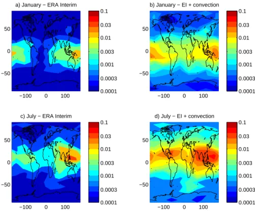
extracted from Eq. (6), is shown in Fig. 1 for January and July for runs with and without convection. The results show
that the injected fraction is always greater when convection is included although runs with and without convection show similar latitude and longitude variations in the tropics where the fraction is largest.
The spatial variation of the emitted species fraction trans-ported to the stratosphere (Fig. 1) shows a dominant source region for air reaching the tropical tropopause region over the equatorial west Pacific region in Northern Hemisphere (NH) winter which moves northward and extends west-wards to include south-east and south Asia in NH summer. This is broadly as expected from previous trajectory studies (Fueglistaler et al., 2004; Berthet et al., 2007) and (for NH winter only) the Eulerian study of Aschmann et al. (2009). The localisation of the source regions for rapid transport to the stratosphere is consistent with current ideas that only out-flow from only the highest convection is likely to ascend into the stratosphere on short time scales (e.g. Fueglistaler et al., 2009, and references therein). Note that the study by Levine et al. (2007) shows less localisation, but they consider trans-port into the stratosphere not only via the tropical tropopause, but also quasi horizontally into the lowermost stratosphere.
To estimate VSLS ODPs, the fraction of halogen injected across the 380 K surface at location y and time s needs to be weighted by the stratospheric residence time Tresstrat(y,s).
This is estimated for every month with an ensemble (2.2 mil-lion) of stratospheric trajectories, on a 2◦×2◦ grid, using a seasonally varying, but perpetual year 2000, wind fields from ERA-Interim. In order to diagnose the time spent dur-ing the first passage through the stratosphere the trajecto-ries were followed for 20 yr, significantly longer than stan-dard estimates of lower stratospheric turnover time. The trajectories were judged to have left the stratosphere when they first crossed the WMO thermal tropopause also deduced from ERA-Interim data. Figure 2 displays Tresstrat(y,s) for
tra-jectories leaving the 380 K surface as a function of starting latitude and month. The results show a clear seasonal cy-cle, with, in the tropics, significant variability in the resi-dence times. Tresstrat(y,s) is shown in Fig. 3 as function of
potential temperature and latitude calculated using ensem-bles of trajectories starting on several different potential tem-perature surfaces. It exhibits a pattern that might be ex-pected from the large-scale stratospheric circulation and in-deed Tresstrat(y,s) is complementary to stratospheric age of air,
which is a more standard and familiar diagnostic of the circu-lation (e.g. Waugh and Hall, 2002). For example, the effect of the tropical pipe can be seen at the Equator above 500 K, with a clear maximum in residence time due to that fact that an air parcel starting at this location will be taken upwards in the tropical pipe before then descending in the extratropics. As discussed in the previous section, the results displayed in Figs. 2 and 3 can be used to estimate a residence time for reactive halogen produced by CFC-11 of about 60 months as-suming that it breaks down in the tropical stratosphere above 20 km ('530 K).
−100 0 100 −50
0 50
a) January − ERA Interim
0.0001 0.0003 0.001 0.003 0.01 0.03 0.1 −100 0 100 −50 0 50 b) January − EI + convection 0.0001 0.0003 0.001 0.003 0.01 0.03 0.1 −100 0 100 −50 0 50
c) July − ERA Interim
0.0001 0.0003 0.001 0.003 0.01 0.03 0.1 −100 0 100 −50 0 50 d) July − EI + convection 0.0001 0.0003 0.001 0.003 0.01 0.03 0.1
Fig. 1. Fraction of accumulated halogen reaching the 380 K surface within one year of a pulse
emission of an nPB-like substance shown as a function of surface location of the emission. The fraction is estimated using forward trajectories started near the surface. Panels a and b correspond to January 2001. Panels c and d correspond to July 2001. Panels a and c use ERA Interim vertical velocities. Panels a and c use ERA Interim with the Emanuel convective parametrization as implemented in FLEXPART 6.2. See text for details.
30
Fig. 1. Fraction of accumulated halogen reaching the 380 K surface within one year of a pulse emission of an nPB-like substance shown
as a function of surface location of the emission. The fraction is estimated using forward trajectories started near the surface. (a) and (b) correspond to January 2001. (c) and (d) correspond to July 2001. (a) and (c) use ERA Interim vertical velocities. (a) and (c) use ERA Interim with the Emanuel convective parametrization as implemented in FLEXPART 6.2. See text for details.
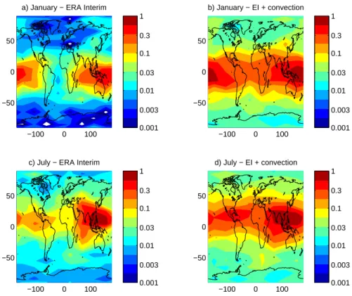
Based on the results from the tropospheric and strato-spheric trajectory calculations, ODPs can be calculated from Eq. (7). Again for illustrative purposes, and consistent with the assumed 20 d lifetime, we consider a VSLS like n-PB as an example with nBr=1, nCl=0, nCl(CFC-11) = 3,
TCFCactive-11=60 months, MCFC-11/MX=137.37/123.0 ' 1 and
α =60. Figure 4 shows the resulting ODP distribution for January and July 2000 as a function of surface emission location, for calculations without and with the convective parametrisation. Including the convective parametrisation enhances ODPs by up to a factor of 2. For example, with the convective parametrisation, ODPs in NH summer ex-ceed 0.6 for emissions over southern Asia and have values of up to 0.2 for emissions over Central America. Maximum values are not significantly changed without the convective parametrisation, but values over the tropics as a whole are somewhat reduced. There is at least a factor of 4 reduc-tion in the longitudinal average in the tropics compared to the extratropics. With the convective parametrisation, sum-mer ODPs of around 0.03 are found for emissions at northern mid-latitudes, e.g. northern Europe, with values in excess of 0.1 for emissions at latitudes corresponding to southern Eu-rope and the northern United States (US). These extratropi-cal values are typiextratropi-cally reduced by a factor of 3 or so in runs
without the convective parametrization. It is worth noting that legislation in the US sets a limit of 0.2 for substances which are not controlled and the US Environmental Protec-tion Agency cauProtec-tions that chemicals with ODPs greater than 0.05 should be considered carefully (Wuebbles et al., 2009). The ODP spatial distribution is similar to that of the quan-tity shown in Fig. 1 in terms of where the maxima are located. This similarity suggests that the effect of spatial variation in the stratospheric residence time is relatively weak. However, it is important to realise that the similarity in spatial distri-bution results primarily from the concentration in the trop-ics and, in particular, this means that it is the stratospheric residence time associated with tropical injection that deter-mines the ODP. Using a global average value (over injection locations) of the stratospheric residence time would underes-timate the ODP by a factor of 2 or so.
As noted for the fraction injected into the stratosphere (Fig. 1) the ODP results also show strong longitudinal varia-tion (factor 3 or more) within the tropics as well as a strong seasonal variations. They suggest that ODPs for emissions from southern Asia in NH summer may be larger than for emissions from the western Pacific in NH winter. In NH summer significant ODP values extend southwards over the Indian ocean well beyond what are generally regarded as
stratospheric residence time from 380 K (month) Month Latitude 1 2 3 4 5 6 7 8 9 10 11 12 −80 −60 −40 −20 0 20 40 60 80 6 8 10 12 14 16 18 20 22 24 26
Fig. 2. Zonally averaged stratosphere residence time (see text) (colour indicates months) for airmasses starting on the 380 K surface as a function of latitude and time of the year of the starting point. Trajectories were integrated using perpetual year 2000 velocity fields from the ERA Interim dataset. See text for details.
31
Fig. 2. Zonally averaged stratosphere residence time (see text)
(colour indicates months) for airmasses starting on the 380 K sur-face as a function of latitude and time of the year of the starting point. Trajectories were integrated using perpetual year 2000 ve-locity fields from the ERA Interim dataset. See text for details.
regions of active convection. This is consistent with the ex-pected northward cross-equatorial flow into the convective regions and emphasises that the spatial distribution of ODPs is determined not only by the location of the most active con-vective regions but also by the pattern of low-level flow into those regions. Note that for the calculation without convec-tion, the maximum ODPs over Asia are not reduced much relative to the calculations with convection but extend over a smaller region. A secondary maxima can also be seen over central America in NH summer.
WMO (2007) (Sect. 2.6.2) give an order of magnitude es-timate for the ODP of a VSLS, such as n-PB, containing one bromine atom and with a molecular weight similar to CFC-11. They estimated that the fraction reaching stratosphere might typically range between 10−3and 10−2for a species with a lifetime of 25 d, according to emission location. Our calculations indicate that this fraction might be as much as 10−1in certain regions (see Fig. 1), and that ODPs might be as large as 0.6 in these regions, as indicated in Fig. 4. Global mean ODPs for the 20 d tracer shown here vary from 0.021 and 0.035 in January and July in runs without convection to 0.067 and 0.079 in runs with convection. Results for different latitude bands for January and July for runs with and without convection are shown in Table 1.
These estimates are generally higher than previous esti-mates for n-PB based on emissions located in northern mid-latitudes (WMO, 2003, 2007). Wuebbles et al. (2001) es-timated n-PB ODPs ranging from 0.033 to 0.040 for emis-sions over land and 0.021 to 0.028 for emisemis-sions over indus-trialized regions in the Northern Hemisphere. More recently, Wuebbles et al. (2009) re-evaluated n-PB OPDs finding val-ues in mid-latitudes of 0.019 based on 2-D model calcula-tions and 0.005 based on a 3-D model. These results, which
year average stratospheric residence time (month)
Latitude Potential temperature (K) −80 −60 −40 −20 0 20 40 60 80 400 420 440 460 480 500 520 10 15 20 25 30 35 40 45 50 55 60
Fig. 3. Latitude-height cross section of stratospheric residence time for trajectories starting at different heights, from 380 K to 540 K, and latitudes. Trajectories were integrated using perpet-ual year 2000 velocity fields from the ERA Interim dataset. See text for details.
32
Fig. 3. Latitude-height cross section of stratospheric residence time
for trajectories starting at different heights, from 380 K to 540 K, and latitudes. Trajectories were integrated using perpetual year 2000 velocity fields from the ERA Interim dataset. See text for details.
Table 1. Estimated ODPs for the nPB-like substance as a function
of emission location, area-averaged over different latitude bands.
Jannoconv Janconv Julnoconv Julconv
60◦N–90◦N 0.0041 0.0143 0.0081 0.0217 30◦N–60◦N 0.0052 0.0266 0.0289 0.0654 30◦S–30◦N 0.1321 0.3027 0.1736 0.3285 30◦S–60◦S 0.0108 0.0333 0.0091 0.0213 60◦S–90◦S 0.0016 0.0114 0.0043 0.0138
are annual means over land surfaces where the substances were emitted, are lower than the results presented in Table 1, especially when convection is taken into account. How-ever, the global model estimates included convection and also a rather detailed treatment of n-PB degradation. They included new kinetic data for the degration of an important n-PB product gas, bromoacetone (BrAc) finding a shorter life-time (around 5 h) compared to previous studies. They esti-mated a lifetime for n-PB of around 24 d using both the 2-D and 3-D models. Wuebbles et al. (2009) also found a factor of 2 difference between mid-latitude (30◦–60◦N) and
trop-ical (20◦S–20◦N) regions for another VSLS, CF
3I. Our
es-timates suggest a much larger difference (factor 5 to 11 in the runs with convection) between tropical and extratropical values. Recently, Wuebbles et al. (2010) have refined these values of ODP for nPB in the band 30◦N–60◦N to 0.0049 and the lifetime to 24.7 days and in the 60◦S–70◦N band a mean of 0.011 with a lifetime of 19.6 days.
The estimates of ODPs shown in Fig. 4 are, of course, dependent on the assumptions underlying the modelling methodology outlined in Sect. 2 and, in particular use of a trajectory-based approach. There is reason to believe that
−100 0 100 −50
0 50
a) January − ERA Interim
0.001 0.003 0.01 0.03 0.1 0.3 1 −100 0 100 −50 0 50 b) January − EI + convection 0.001 0.003 0.01 0.03 0.1 0.3 1 −100 0 100 −50 0 50
c) July − ERA Interim
0.001 0.003 0.01 0.03 0.1 0.3 1 −100 0 100 −50 0 50 d) July − EI + convection 0.001 0.003 0.01 0.03 0.1 0.3 1
Fig. 4. Ozone Depletion Potentials for the nPB-like (20 d lifetime) substance as a function
of latitude and longitude of emission location. Panels a and b correspond to January 2001. Panels c and d correspond to July 2001. Panels a and c use ERA Interim vertical velocities. Panels a and c use ERA Interim with the Emanuel convective parametrization as implemented in FLEXPART 6.2.
33
Fig. 4. Ozone Depletion Potentials for the nPB-like (20 d lifetime) substance as a function of latitude and longitude of emission location. (a)
and (b) correspond to January 2001. (c) and (d) correspond to July 2001. (a) and (c) use ERA Interim vertical velocities. (a) and (c) use ERA Interim with the Emanuel convective parametrization as implemented in FLEXPART 6.2.
trajectories based on large-scale wind fields alone underes-timate rapid vertical transport in the tropics. For example, Law et al. (2010) have suggested that use of such trajecto-ries underestimates the contribution of deep convection over Asia to the air masses in the tropical tropopause layer (TTL) observed over west Africa and estimates of convective trans-port based on trajectories calculated explicitly in a meso-scale model appear to show deeper transport of air masses into the tropical tropopause layer (Fierli et al., 2010). The inclusion of the convective parameterization in the FLEX-PART trajectory code clearly has a significant impact on our results and may go some way to improving the representation of transport based on large-scale trajectories alone. Never-theless, large uncertainties remain and it would be interest-ing to repeat the present experiment with different convec-tive parametrisations. Wuebbles et al. (2010) used MOZART driven by CCM3 winds. Moist convection in the CCM3 in-cludes the deep convection scheme developed by Zhang and McFarlane (1995) which operates in conjunction with the scheme of Hack (1994). Tost et al. (2010) compared different convective parametrisation schemes in a global CTM, show-ing that the choice of the convection parametrisation in a global model of the chemical composition of the atmosphere has a substantial influence on trace gas distributions. In Fig. 2 of Tost et al. (2010), it is apparent that Emanuel parametri-sation injects more mass across the 250 mb surface in the
tropics than the scheme of Zhang and McFarlane. For exam-ple panel b shows differences of the order of 100% for222Rn between Zhang and McFarlane and Emanuel above 200 mb.
Increased injected mass across the 380 K surface in the tropics may be among the causes for the larger ODP esti-mates in the tropics here relative to Wuebbles et al. (2009, 2010) in addition to uncertainties related to the treatment of both tropospheric and stratospheric chemistry. It is worth re-marking that the divergences appear mainly within the trop-ical belt and with the Emanuel parametrisation since our values for midlatitudes driven with ERA Interim winds and those in Wuebbles et al. (2009, 2010) are of a compara-ble order of magnitude. The assumptions related to strato-spheric chemistry also introduce limitations for the accurate calculation of ODPs and may also explain some of the dif-ferences between our estimates and other numbers found in the literature. Another possible cause is an underestimation of the total ozone destroyed by CFC-11. In fact, CFC ef-fect in the stratosphere is estimated using a full description of the stratospheric turnover of the injected masses yield-ing an expected residence time dependyield-ing on the latitude and height, rather than a simple global mean residence time. CFC-11 is modelled as being activated above 30 hPa, but at this height the expected residence estimated is rather a lower boundary since we have used a 20 year trajectory calculation and at this height trajectories may remain in the stratosphere
for longer periods. A full assessment of the stratospheric expected residence time and age of stratospheric air would be advisable to address such an uncertainty. Eulerian model studies such as Wuebbles et al. (2009, 2010) may not have made such approximations of the stratospheric chemistry. In the real stratosphere, the amount of ozone destroyed by chlorine/bromine will not just depend linearly on the time spent in the stratosphere. If an air parcel reaches a high alti-tude, where the photochemical lifetime of ozone is short then ozone will reach equilibrium. In addition, bromine chemistry is not so efficient at these altitudes (WMO, 2007; Salaw-itch et al., 2005). In our approach, the different activation heights of chlorine from CFC-11 (above 30 hPa) and bromine from VSLS (above 380 K) aims to represent the inhomoge-neous distribution of active species and other factors influ-encing the depletion reactions. The chlorine from CFC-11 and bromine from VSLS released is then modelled as re-maining active along the transit through the stratosphere until the parcel under consideration is expelled back into the tro-posphere. This approximation largely neglects effects arising from the inhomogeneous distribution of active (radical) and inactive (reservoir) halogen; instead, only a mean efficiency factor α published in the literature (WMO, 2003, 2007) was assumed. This assumption could be relaxed in future studies but would add significant computational costs from running box models along the stratospheric trajectories.
The prediction of higher fractions of VSLS emissions reaching the stratosphere in NH summer, in particular, from southern Asia, than in NH winter, and the correspondingly higher ODPs for tropical emissions in NH summer versus those in NH winter is interesting. There are hints of this in previous results, e.g. results from the 1-D model study of Gettelman et al. (2009) show CO values that are larger in the lower stratosphere for NH summer over southern Asia than for NH winter over the west Pacific. However, this difference may arise from differences in the lower stratospheric circu-lation rather than from differences in vertical transport in the troposphere. Of course there have been many previous stud-ies which highlight the strong differences between NH sum-mer and NH winter, but it is important to keep in mind the precise measure of the circulation that is being considered. Fueglistaler et al. (2004, 2005) showed the low-level source region for air that subsequently reaches the stratosphere (and therefore determines stratospheric water vapour), but there was no particular criterion on transport timescale. Several studies have emphasised the role of the NH summer Asian monsoon anticyclone, with the relative isolation in the in-terior of the upper anticyclone leading to coherent features in water vapour (e.g. James et al., 2008) and in a variety of chemical species including CO, HCN, C2H6 and C2H2
(Park et al., 2008). Indeed Randel et al. (2010) have used HCN measurements to argue for a special role for the Asian monsoon anticyclone system in bringing polluted air from the south and east Asian region to the stratosphere in NH summer. However modelling studies such as Li et al. (2009)
suggest that sources over a much broader geographical re-gion are responsible for HCN variations. In any case HCN has a multi-year photochemical lifetime and an oceanic sink. Independent verification of the seasonal variations shown in Figs. 1 and 3 is more likely to come from observations of short-lived species such as Acetylene (C2H2), but the effects
of seasonal variations in convective transport would have to be distinguished from seasonal variations in surface emis-sions.
The results presented here consider only the effect of trajectories that penetrate above 380 K. It has been noted (Levine et al., 2007) that there may be significant ozone de-pletion in the lowermost stratosphere due to VSLS and their product gases which are transported quasi-horizontally into the lowermost stratosphere. This could be included in our estimates by adopting a different definition of the control surface ∂. However, we note that residence times within the lower stratosphere are likely to be no more than a few months (compared with the 15 months for air transported across 380 K). Additionally, the results presented in Berthet et al. (2007) suggest that transport into the lowermost strato-sphere in NH winter may be significantly less than that esti-mated by Levine et al. (2007).
Another potential sensitivity in our calculations is the as-sumption of a uniform decay rate λ for total halogen. As noted previously, this represents a combination of photo-chemical destruction of SG and loss of PGs through photo-chemical degradation and washout. If removal of total halogen in the upper troposphere is overestimated through this assumption then ODPs might be larger than estimated here. Certainly transport timescales in the tropical upper troposphere appear to be relatively long, e.g., Kr¨uger et al. (2009) estimate, on the basis of trajectory calculations similar to those used in this paper, that the time to ascend from 360 K to 380 K may be 30 d or more, though, as noted previously, deep convec-tion over particular regions may penetrate high into the TTL (Fierli et al., 2010) thereby reducing transport timescales. In the case that air resides for 30 d or more in the TTL, our as-sumption of 20 d exponential decay would imply significant reduction in total halogen before reaching 380 K. The lat-ter reduction in total halogen might well be an overestimate since, if convective penetration into this region is relatively rare, then removal by washout in this region is likely to be slow. On the other hand there is also the possibility of re-moval of total halogen through uptake on thin cirrus clouds which form as part of the process of dehydration of air as it enters the stratosphere (Sinnhuber and Folkins, 2006).
4 Conclusions
Calculating ODPs for VSLS is challenging because the ODPs are expected to be strong functions of location and time of emission, implying the need for many calculations with different emission distributions. Ultimately, multiple
calculations are needed with global 3-D models that repre-sent both the tropospheric chemistry and transport processes that determine what fraction of the emitted halogen reaches the stratosphere, plus the stratospheric chemistry and trans-port processes that determine the resulting ozone depletion, but currently these are computationally expensive. Up to now ODP estimates have usually been based on simplified approaches that, for example, follow tropospheric evolution in some detail to predict the fraction of the halogen reaching the stratosphere, followed by some kind of approximate cal-culation of the implied ODP (e.g., Bridgeman et al., 2000; Olsen et al., 2000; Wuebbles et al., 2001). The exception is Wuebbles et al. (2009, 2010) which used a 3-D model of both troposphere and stratosphere.
Here, we have set out a trajectory-based methodology that gives the ODP as a function of location and time of emis-sion. We believe the trajectory-based calculation to be as good a representation of tropospheric transport processes as an Eulerian CTM, not least because it is based on the same sort of velocity dataset that is typically used for an Eulerian calculation. The stratospheric calculation makes similar ap-proximations to those that have been used before to estimate ODPs and indeed for long-lived species we see some advan-tage to our approach since it requires integration not for the lifetime of the emitted species but only for the time required to estimate the stratospheric residence time of the resulting active species. Furthermore, the separation of the calculation into tropospheric and stratospheric parts allows significant computational saving.
The calculations presented here are based on the simplest possible representation of tropospheric chemistry. Therefore, the primary interest in the results is not so much the absolute value of the ODPs but the implied spatial and temporal vari-ation. The results shown in Fig. 4 show clearly that not only is there strong latitudinal variation, as has been suggested by previous work, but also that there is very significant longi-tudinal and seasonal variation. This is not unexpected from previous analysis of transport in the tropical troposphere, but our results are, we believe, the first quantitative estimates of implications for ODPs. The estimated ODPs are much higher than previous estimates in certain localised regions. (A re-cent paper by Brioude et al. (2010), submitted after this pa-per, includes a more detailed representation of tropospheric chemistry and suggests that our 20 day timescale for n-PB may be too long, implying that our estimated numerical val-ues of ODPs should be smaller. But the strong dependence on location and season of the source is also found by Brioude et al. (2010), albeit in a less detailed analysis which does not include any analogue of our Fig. 4 showing ODP as a func-tion of posifunc-tion.)
Extension to more sophisticated tropospheric or strato-spheric chemistry would be possible without recalculation of the large trajectory dataset on which the estimates are based. Existing chemical trajectory codes could be used for both tropospheric and stratospheric parts of the calculation, with
background chemical fields taken from a suitable Eulerian CTM. Representation of removal by moist processes would also be relatively straightforward to incorporate. The sen-sitivity demonstrated here of the estimated ODPs to the in-clusion of convective parametrization emphasises the current quantitative uncertainty over precise values of ODPs. Even if it is accepted that a convective scheme is necessary the estimated values are likely to be depend on which particu-lar convective scheme is chosen and any communication of ODPs to policymakers needs to emphasise the range of un-certainty associated with representation of convection or of any other processes.
Space and time integrals of the calculated ODP distri-butions, can be calculated straightforwardly to give overall ODPs for many different emissions scenarios. This would allow estimation of, for example, regional ODPs or ODPs for particular ship or aircraft routes. Detailed tables (large arrays) could be easily produced for automated evaluation for the use of policymakers.
Extension to different halogen-containing species (chlo-rinated, brominated, iodinated) would also be straightfor-ward using different values of α or with a more sophisti-cated chemistry schemes. In particular, it would be possi-ble to calculate ODPs for naturally occuring bromine species emitted by the tropical ocean (see e.g. Warwick et al., 2006) and to consider, for example, how the ODPs change as trop-ical ocean temperatures change in the future (e.g. consider-ing the wind fields from a climate model). Correspondconsider-ingly, ODPs for new artificial halogenated species could be esti-mated, given knowledge of their emissions, which might re-sult from manufacture, use and disposal. NH midlatitudes have conventionally been seen as likely source regions for such species and ODPs would then be correspondingly small. But emissions resulting form continuing industrialisation and population growth in south and south-east Asia would clearly from Fig. 4 have a much larger potential impact on strato-spheric ozone. This focuses attention on the precise spatial variation of the ODP distribution in this region and its re-lation to convecting regions. The pattern of low-level inflow into the Asian monsoon and its relation to potential emissions is a crucial aspect requiring further investigation.
Acknowledgements. This work was supported by the EU SCOUT-O3 Integrated Project (GOCE-CT-2004505390). We thank Gavin Esler, Stephan Fueglistaler, Sue Liu and Kirstin Kr¨uger for useful discussions. Part of the calculations were performed using CICLAD, the computing system of IPSL.
The publication of this article is financed by CNRS-INSU.
References
Aschmann, J., Sinnhuber, B.-M., Atlas, E. L., and Schauffler, S. M.: Modeling the transport of very short-lived substances into the tropical upper troposphere and lower stratosphere, Atmos. Chem. Phys., 9, 9237–9247, doi:10.5194/acp-9-9237-2009, 2009. Berthet, G., Esler, J. G., and Haynes, P. H.: A Lagrangian
perspective of the tropopause and the ventilation of the lowermost stratosphere, J. Geophys. Res., 112, D18102, doi:10.1029/2006JD008295, 2007.
Bridgeman, C. H., Pyle, J. A., and Shallcross, D. E.: A three-dimensional model calculation of the ozone depletion potential of 1-bromopropane (1-C3H7Br), J. Geophys. Res., 105, 26493– 26502, 2000.
Brioude, J., Portmann, R. W., Daniel, J. S., Cooper, O. R., Frost, G. J., Rosenlof, K. H., Granier, C., Ravishankara, A. R., Montzka,S. A. and Stohl, A.: Variations in ozone de-pletion potentials of very short-lived substances with sea-son and emission region. Geophys. Res. Lett., 37, L19804, doi:10.1029/2010GL044856, 2010.
Butler, J. H., King, D. B., Lobert, J. M., Montzka, S. A., Yvon-Lewis, S. A., Hall, B. D., Warwick, N. J., Mondeel, D. J., Ay-din, M., and Elkins, J. W.: Oceanic distributions and emissions of short-lived halocarbons, Global Biogeochem. Cy., 21, GB1023, doi:10.1029/2006GB002732, 2007.
Dorf, M., Butz, A., Camy-Peyret, C., Chipperfield, M. P., Kritten, L., and Pfeilsticker, K.: Bromine in the tropical troposphere and stratosphere as derived from balloon-borne BrO observations, Atmos. Chem. Phys., 8, 7265–7271, doi:10.5194/acp-8-7265-2008, 2008.
Fierli, F., Orlandi, E., Law, K. S., Cagnazzo, C., Cairo, F., Schiller, C., Borrmann, S., Didonfrancesco, G., Ravegnani, F., and Volk, M.: Impact of deep convection in the tropical tropopause layer in West Africa: in-situ observations and mesoscale modelling, At-mos. Chem. Phys. Discuss., 10, 4927–4961, doi:10.5194/acpd-10-4927-2010, 2010.
Forster, C., Stohl, A., and Seibert, P.: Parameterization of con-vective transport in a Lagrangian particle dispersion model and its evaluation, J. Appl. Meteorol. Climatol., 46, 403–422, doi:10.1175/JAM2470.1, 2007.
Fueglistaler, S., Wernli, H., and Peter, T.: Tropical troposphere-to-stratosphere transport inferred from trajectory calculations, J. Geophys. Res., 109, D03108, doi:10.1029/2003JD004069, 2004. Fueglistaler, S., Bonazzola, M., Haynes, P. H., and Peter, T.: Strato-spheric water vapor predicted from the Lagrangian temperature history of air entering the stratosphere in the tropics, J. Geophys. Res., 110, D08107, doi:10.1029/2004JD005516, 2005.
Fueglistaler, S., Dessler, A. E., Dunkerton, T. J., Folkins, I., Fu, Q., and Mote, P. W.: Tropical tropopause layer, Rev. Geophys., 47, RG1004, doi:10.1029/2008RG000267, 2009.
Gettelman, A., Lauritzen, P. H., Park, M., and Kay, J. E.: Processes regulating short-lived species in the tropical tropopause layer, J. Geophys. Res., 114, D13303, doi:10.1029/2009JD011785, 2009. Hack, J. J.: Parameterization of moist convection in the National Center for Atmospheric Research Community Climate Model (CCM2), J. Geophys. Res., 99, 5551–5568, 1994.
Hossaini, R., Chipperfield, M. P., Monge-Sanz, B. M., Richards, N. A. D., Atlas, E., and Blake, D. R.: Bromoform and dibro-momethane in the tropics: a 3-D model study of chemistry and transport, Atmos. Chem. Phys., 10, 719–735, doi:10.5194/acp-10-719-2010, 2010.
James, R., Bonazzola, M., Legras, B., Surbled, K., and Fueglistaler, S.: Water vapor transport and dehydration above convective outflow during Asian monsoon, Geophys. Res. Lett., 35, L20810, doi:10.1029/2008GL035441, 2008.
Kerkweg, A., J¨ockel, P., Pozzer, A., Tost, H., Sander, R., Schulz, M., Stier, P., Vignati, E., Wilson, J., and Lelieveld, J.: Consistent simulation of bromine chemistry from the marine boundary layer to the stratosphere – Part 1: Model description, sea salt aerosols and pH, Atmos. Chem. Phys., 8, 5899–5917, doi:10.5194/acp-8-5899-2008, 2008a.
Kerkweg, A., J¨ockel, P., Warwick, N., Gebhardt, S., Brenninkmei-jer, C. A. M., and Lelieveld, J.: Consistent simulation of bromine chemistry from the marine boundary layer to the stratosphere – Part 2: Bromocarbons, Atmos. Chem. Phys., 8, 5919–5939, doi:10.5194/acp-8-5919-2008, 2008b.
Kr¨uger, K., Tegtmeier, S., and Rex, M.: Variability of resi-dence time in the Tropical Tropopause Layer during North-ern Hemisphere winter, Atmos. Chem. Phys., 9, 6717–6725, doi:10.5194/acp-9-6717-2009, 2009.
Law, K. S., Fierli, F., Cairo, F., Schlager, H., Borrmann, S., Streibel, M., Real, E., Kunkel, D., Schiller, C., Ravegnani, F., Ulanovsky, A., D’Amato, F., Viciani, S., and Volk, C. M.: Air mass origins influencing TTL chemical composition over West Africa during 2006 summer monsoon, Atmos. Chem. Phys., 10, 10753–10770, doi:10.5194/acp-10-10753-2010, 2010.
Legras, B., Joseph, B., and Lef`evre, F.: Vertical diffusivity in the lower stratosphere from Lagrangian back-trajectory recon-structions of ozone profiles, J. Geophys. Res., 108, 4562, doi:10.1029/2002JD003045, 2003.
Levine, J., Braesicke, P., Harris, N. R. P., Savage, N. H., and Pyle, J. A.: Pathways and timescales for troposphere to-stratosphere transport, J. Geophys. Res., 112, D04308, doi:10.1029/2005JD006940, 2007.
Li, Q., Palmer, P. I., Pumphrey, H. C., Bernath, P., and Mahieu, E.: What drives the observed variability of HCN in the tropo-sphere and lower stratotropo-sphere?, Atmos. Chem. Phys., 9, 8531– 8543, doi:10.5194/acp-9-8531-2009, 2009.
Olsen, S., Hannegan, B. J., Zhu, X., and Prather, M.: Evaluat-ing ozone depletion from very short-lived halocarbons, Geophys. Res. Lett., 27, 1475–1478, 2000.
Park, M., Randel, W. J., Emmons, L. K., Bernath, P. F., Walker, K. A., and Boone, C. D.: Chemical isolation in the Asian monsoon anticyclone observed in Atmospheric Chemistry Ex-periment (ACE-FTS) data, Atmos. Chem. Phys., 8, 757–764, doi:10.5194/acp-8-757-2008, 2008.
Randel, W. J., Park, M., Emmons, L., Kinnison, D., Bernath, P., Walker, K. A., Boone, C., and Pumphrey, H.: Asian monsoon transport of pollution to the stratosphere, Science, 328, 611–613,
2010.
Salawitch, R. J., Weisenstein, D. K., Kovalenko, L. J., Sioris, C. E., Wennberg, P. O., Chance, K., Ko, M. K. W., and McLinden, C. A.: Sensitivity of ozone to bromine in the lower stratosphere, Geophys. Res. Lett., 32, L05811, doi:10.1029/2004GL021504, 2005.
Sinnhuber, B.-M. and Folkins, I.: Estimating the contribution of bromoform to stratospheric bromine and its relation to dehydra-tion in the tropical tropopause layer, Atmos. Chem. Phys., 6, 4755–4761, doi:10.5194/acp-6-4755-2006, 2006.
Solomon, S. and Albritton, D. L.: Time dependent ozone depletion potentials for short- and long-term forecasts, Nature, 357, 33–37, 1992.
Solomon, S., Mills, M., Heidt, L. E., Pollock, W., and Tuck, A. F.: On the evaluation of ozone depletion potentials, J. Geophys. Res., 97, 824–842, 1992.
Stohl, A., Forster, C., Frank, A., Seibert, P., and Wotawa, G.: Technical note: The Lagrangian particle dispersion model FLEXPART version 6.2, Atmos. Chem. Phys., 5, 2461–2474, doi:10.5194/acp-5-2461-2005, 2005.
Tost, H., Lawrence, M. G., Br¨uhl, C., J¨ockel, P., The GABRIEL Team, and The SCOUT-O3-DARWIN/ACTIVE Team: Uncer-tainties in atmospheric chemistry modelling due to convection parameterisations and subsequent scavenging, Atmos. Chem. Phys., 10, 1931–1951, doi:10.5194/acp-10-1931-2010, 2010. Warwick, N. J., Pyle, J. A., Carver, G. D., Yang, X.,
Sav-age, N. H., O’Connor, F. M., and Cox, R. A.: Global model-ing of biogenic bromocarbons, J. Geophys. Res., 111, D24305, doi:10.1029/2006JD007264, 2006.
Waugh, D. W. and Hall, T. M.: Age of stratospheric air: the-ory, observations, and models, Rev. Geophys., 40(4), 1010, doi:10.1029/2000RG000101, 2002.
WMO: Scientific Assessment of Ozone Depletion: 2002, Tech. Rep. 47, World Meteorological Organization, Geneva, 2003. WMO: Scientific Assessment of Ozone Depletion: 2006, Tech.
Rep. 50, World Meteorological Organization, Geneva, 2007. Wuebbles, D. J.: Chlorocarbon emission scenarios: potential
im-pact on stratospheric ozone, J. Geophys. Res., 88, 1433–1443, 1983.
Wuebbles, D. J., Patten, K., Johnson, M., and Kotamarthi, R.: New methodology for ozone depletion potentials of short-lived com-pounds: n-propyl bromide as an example, J. Geophys. Res., 106, 14551–14571, 2001.
Wuebbles, D. J, Youm, D., Patten, K., and Avil´es, M. M.: Met-rics for Ozone and Climate: Three-Dimensional Modeling Stud-ies of Ozone Depletion Potentials and Indirect Global Warm-ing Potentials, in: Twenty Years of Ozone Decline, 297–326, doi:10.1007/978-90-481-2469-5 23, 2009.
Wuebbles, D. J., Patten, K. O., Wang, D., Youn, D., Mart´ınez-Avil´es, M., and Francisco, J. S.: Three-dimensional model eval-uation of the Ozone Depletion Potentials for n-propyl bromide, trichloroethylene and perchloroethylene, Atmos. Chem. Phys. Discuss., 10, 17889–17910, doi:10.5194/acpd-10-17889-2010, 2010.
Zhang, G. J. and McFarlane, N. A.: Sensitivity of climate simula-tions to the parameterization of cumulus convection in the Cana-dian Climate Centre general circulation model, Atmos.-Ocean, 33, 407–446, 1995.