Distribution-Free, Uniformly-Tighter Linear Approximations for Chance-Constrained Programmingt
Gabriel R. Bitran* Thin-Yin Leong**
MIT Sloan School Working Paper #3111-90-MSA
January 1990
* Massachusetts Institute of Technology Sloan School of Management
Cambridge, MA 02139 ** Sloan School of Management and National University of Singapore
Republic of Singapore
tThis research has been partially supported by the Leaders for Manufacturing Program
Distribution-Free, Uniformly-Tighter Linear Approximations+ for Chance-Constrained Programming
Gabriel R. Bitran* and Thin-Yin Leong**
Abstract
We propose a class of deterministic linear approximations to mathematical programs with individual chance constraints. In these approximations, we replace each chance constraint by a set of linear
inequalities. The linear inequalities approximate the chance constraint as opposed to methods that approximate the variance of the chance constraint. This allows us to provide near-optimal solutions of chance-constrained problems that have random variables with arbitrary distributions; the random variables can be dependent.
If the feasible region defined by a chance constraint is convex, we show that the linear approximation is uniformly tighter than the constraint it replaces: any solution to the approximation is feasible to the original constraint. At the cost of doing more work, the number of linear
inequalities can be infinitely increased to make the approximation exact. As examples, we present three simple methods from this class of linear approximations. The computation results show that these approximations work well when the number of random variables is small. The methods can
potentially be applied to production problems where planning is done on a rolling horizon basis.
*Sloan School of Management, Massachusetts Institute of Technology, Cambridge, MA 02139.
**Sloan School of Management, and National University of Singapore, Republic of Singapore.
+This research was partially supported by "The Leaders for Manufacturing Program".
Distribution-Free, Uniformly-Tighter Linear Approximations for Chance-Constrained Programming
Gabriel R. Bitran and Thin-Yin Leong
1. Introduction
In this paper, we present a class of linear approximations to chance-constrained problems where the random variables have arbitrary
distributions. We focus on chance-constrained linear programs (LP) with stochastic technology coefficients--coefficients on the left-hand-side of a constraint. However, the method can also be applied to mathematical
programs that have chance-constrained nonlinear inequalities with stochastic or deterministic resource parameters, the right-hand-side parameter of a constraint. These problems appear in service constrained applications that have uncertainties in the yield or demand. The broad classification of these applications are problems (a) with carry-over resources (inter-period constraints), (b) with portfolio selection (intra-period constraints), and (c) with both carry-over resources and portfolio selection.
Applications of the first type can be found in the areas of production planning and inventory control; facility location planning; project planning (PERT); financial investment planning; cash management; cost-volume-profit analysis; and environmental, public services, and utilities (hospital staffing, reservoir capacity, rail-road system, solid waste system) planning. Portfolio-selection applications include problems in investment portfolio management, activity analysis and technology planning, capital budgeting, animal and human dietary planning, and material composition selection. The lists are not intended to be comprehensive but illustrates the variety of applications. For more
1
applications and detail of specific problems, see [Hogan, Morris, and Thompson 19813.
In general, chance-constrained programs with random technical coefficients are hard to solve. To make the problem tractable, it is
typical to assume that the random coefficients are normally distributed. We propose, in this paper, a new alternative approach. The method relaxes the assumptions needed for the probability distributions of the random
coefficients. Our main goal is to derive an approach that is intuitive and allows easy extraction of a problem's structural properties for building simple effective heuristics.
In this paper, we present three simple methods from our class of approximations. These methods are particularly suited to problems with a small number of random coefficient in a chance constraint. However, in some problems, the structural properties of the problem may permit large n. For example, in production/inventory problems, the service constraints for the planning horizon have a block triangular structure. The chance
constraints with few variables are the service constraints for the more immediate periods; the periods further into the horizon have more
variables. Thus when the planning is done on a rolling horizon basis, the large errors for the periods further away are not important as long as the nearer periods are well approximated. Examples of applying the methods
appear in our earlier work: [Bitran and Leong 1989a], --- 1989b],
[---1989c].
The paper is organized as follows. Section 2 reviews the work of other researchers. Section 3 describes the general principle of our approach and illustrates it with some examples. In section 4, we
recapitulate the equations used in the major alternative approximations and test our method against them. We report the results in section 5 with
comments on extensions and future research. In the last section, we conclude with a short summary.
2. Literature Review and Important Results
(For a quick tutorial on stochastic programming problems and chance-constrained programs, we refer the reader to the introductory comments in [Hillier 1967] and the references mentioned there. Greater details on the subject can be found in stochastic programming texts like [Sengupta 1972], [Vadja 1972], [Kall 1976], and [Dempster 1980].)
Under the condition that the joint distribution function of the random variables is continuous, Symonds [1967] proved that the feasible region of a chance-constrained program can be replaced by a deterministic
equivalent. He also provided results for linear chance-constrained problems where only the resource vector is random. Problems with random resource are
quite well covered in the literature. In fact, most of the research on chance-constrained problems has centered on the cases where only the resource is random. The reader is directed to see [Charnes, Cooper, and Symonds 1958] and [Charnes and Cooper 1963] for more details. In a LP with
stochastic technology coefficients, a chance constraint comprises a linear combination of random variables. The weights used for combining the random variables are the decision variables of the program. Hence in general, before solving the program, the probability of violating the resource capacity is difficult to evaluate.
To simplify the discussion, without loss of generality, we assume that the resource parameter is deterministic. Problems with stochastic resource parameters in the chance constraints can be transformed by
multiplying the parameters with dummy decision variables, thus converting them into technology coefficients. Adding new constraints to the problem,
we set the value of these dummy variables to one. Now consider the chance-constrained linear inequality
Prob(Eni=1 ai xi b) > . (1)
ai, i=l,..,n, are the random technology coefficient variables with
continuous joint distribution; xi, i=l,..,n, are the decision variables; b
is the deterministic resource parameter; and a e [0,1, the service
performance target, is the probability that ni=1 ai xi b is satisfied.
The random variables ai, i=l,..,n, are assumed to have finite mean Eai] and finite variance V[ai = oi2.
By Symonds' theorem, constraint (1) has a deterministic equivalent
g(x) < b, (2)
with vector x _ (x1,..,xn). In general, g(x) is a nonlinear function and
can be written as
g(x) = E[Eni=1 ai xi] + za (V[Eni=1 ai xi])1/2, (3)
where za = z(x), the safety factor, is a function of the service target a as well as the decision vector x. When ai, i=l,..,n, are independent and
normally distributed, (3) becomes
g(x) = Eni=1E[ai] Xi + Z [Eni=1 i2 xi2]1/2 . (4)
Here Z is the "one-tail" normal variate for a and depends on a only. This value can be obtained easily from the tables in most basic statistics texts. () is true because a linear combination of normal random variables is also normally distributed.
The representation in (4) is also applicable to the class of stable probability distributions (see [Allen, Braswell, and Rao 1974]). Stable distributions are distributions, completely specified by their means and
standard deviations, such that a linear combination of random variables with a common stable distributional form has the same distributional form. It is not necessary for the random variables to be identically distributed. Their means and variances may be different but they must be from a common distributional form. The class of stable distributions include the normal, Poisson, Chi-square, and binomial distributions. Though not as readily available as the normal variate, the safety factor for the other stable distributions can be computed or found in published tables. Again, the safety factor for stable distributions is independent of the decision variables: the safety factor is a function of a only.
CONDITION Cl: Random variables ai, i=l,..,n, share a common stable
distributional form.
When condition C1 is true and the random variables are dependent, za is still a function of a only. However, in general, since za may be
dependent on x, g(x) is difficult to evaluate and usually cannot be expressed in closed form.
THEOREM1 Kataoka 19631: A chance-constrained linear inequality under C1 and with za 0 is convex. ·
Theorem 1 is the main published result on the convexity of a
chance-constrained linear inequality. Little is known to date about the convexity of (1) when the random variables are of other distributions. Hillier 1967] mentioned that for arbitrary distributions, under fairly weak conditions, the central limit theorem may permit the normal approximation. Charnes,
Cooper, and Thompson [1963] suggested that a mixture of normal
distributions can be used to approximate distributions of fairly arbitrary shapes. Under this approximation, the term ni=l ai Xi in (1) is again a normal random variable. Za, the safety factor for the normal distribution, is non-negative when a 0.5. Therefore, using theorem 1, we can argue that
for a 0.5, (1) is usually convex. Our simulation experiments, on common distributions, indicate that for a close to 1, (1) is convex. We did not find any general theoretical result on the neccessary conditions for convexity of (1). Some work in this area has been done by Prekopa [1971,1974]. This remains an interesting research question for further study.
ASSUMPTION A: The feasible region of (1) is convex. ·
We will assume Al to be true for the rest of this paper. This condition has been assumed to be true in almost all the work we came across. Hence the assumption we make is no more restrictive than those that have been made (see for example, [Hillier 19673 and [Seppald 19713).
The usual approach taken by previous studies, after assuming Cl and convexity (Al), is to solve the chance-constrained problem with nonlinear programming methods. The nonlinear programming methods usually linearize
the problem and search along subgradients. An example of this is Kelly's [1960] cutting plane method. This method solves chance-constrained
programs, in multiple passes, as linear programs. A linear program is first solved without the chance constraints. At each subsequent iteration, a hyperplane tangent to each chance constraint is defined using the preceding iteration's solution and its partial derivatives. These are introduced into the program as additional linear constraints. Prekopa 1988] summarizes the numerical approaches available for solving chance-constrained problems. These nonlinear programming methods tend to be complicated: they require partial derivatives, multiple-pass techniques, and non-standard computer codes. Moreover, they are usually restricted to cases under condition Cl.
Allen, Braswell, and Rao [1974] developed methods for approximating a chance-constrained set using information derived from sample data only. This approach is based on Wilks's [1963] work on the use of statistically
equivalent blocks to construct 1Oa% tolerance regions. The level of confidence of satisfying the chance constraints can be determined from the size of the sample. In addition to the type-one error information implicit in the chance-constraints, this approach gives the decision-maker type-two error information. The paper compared the percentages of empirical
constraint satisfaction of the actual feasibility region by (a) assuming stable distribution, (b) using a safety factor derived from Chebyshev's inequality, (c) using a simple linear approximation, and (d) using a
hyperspherical approximation. Charnes, Kirby, and Raike [19701 studied this further and developed the "acceptance region theory".
Allen, Braswell, and Rao's approximations are not uniformly tighter than the original constraint; the solutions to their approximations are not necessarily feasible to the original problem. However, since the uniformly-tighter characteristic is important in many practical applications of chance-constrained programs, Hillier [1967] and later Seppald [1971, 1972] devised approaches that satisfy that condition. Both methods require
condition C1. In this section, we give a brief sketch of these two methods. We provide their technical detail in section .
Hillier restricted his study to cases where the decision variables are (a) 0-1, (b) 0 or 1, or (c) bounded. He approximated the variance term in (3) with a separable nonlinear function. The separability property of the approximation makes it easier to apply nonlinear programming
techniques. The nonlinear approximation can also be further approximated with a piecewise-linear function using a standard approach in separable convex programs ([Bradley, Hax, and Magnanti 1977]). The piecewise-linear approximation is uniformly tighter than the nonlinear approximation; in turn, the nonlinear approximation is uniformly tighter than the chance
constraint.
7
Despite the set-back of not getting the exact optimal solution, Hillier expounded on the value of linear approximations. The advantages he listed are (a) the relatively high efficiency of solving linear programs, (b) the ability to do sensitivity analysis, and (c) the availability of linear duality theory for analyzing the solutions for managerial
implications. The service levels in the chance constraints may be initially selected by managerial policy. After solving the problem, the service
levels should be re-evaluated against their corresponding optimal dual variable values. These give a measure of the costs of maintaining the
corresponding service levels and hence provide guidance for revising them. Seppdla [1971] relaxed the restrictions, on the decision variables, required by Hillier. Focussing, as in Hillier's approach, on the variance term of the deterministic equivalent (3), Seppdla introduced new variables to break this nonlinear variance term into simpler nonlinear functions. Each nonlinear function is a function of two variables only. He then approximated each of these by piecewise-linear segments. The resulting
linear approximation is uniformly tighter than the chance constraint. In this, as well as Hillier's approach, the decision-maker can choose the number of linear constraints to use to replace the chance constraint. As the number of linear constraints increases, the error of Seppdla's solution
from the optimum approaches zero. For Hillier's method, the error will decrease with more linear constraints but may not go to zero.
In a recent paper, Olson and Swenseth [1987] suggested the simple approximation of replacing each random coefficient ai, i=l,..,n, in (1) by the sum of its expected value and its standard deviation multiplied by a safety factor, shown below:
g(x) = ni=l(E[ai] + Za ai) Xi . (5)
Assuming Cl and with the means and the variances given, this approximation is the same as Allen, Braswell, and Rao's [1974] linear approximation. As an illustration, Olson and Swenseth solve Van de Panne and Popp's [19631 cattle-feed mix problem--assuming independent normal distributions--and
showed that the errors are small.
The details of this approximation is given later. Briefly, this linear approximation consists of only one inner-linearization hyperplane. For the convex case (Al), the hyperplane defines a half space that
guarantees feasibility to (1). Since the feasible region defined by a chance constraint is nonlinear, in the worst case the gap from optimality can be very large. This is particularly so when the magnitudes of the variances relative to the means of the random variables are huge. The
coefficients of variation (COV) in the cattle-feed mix problem are extremely small--less than 0.01--and hence the excellent results.
In cases where condition Cl is not true, both Hillier and Seppdlg suggest that the Chebyshev's inequality be used to obtain the safety
factor. However, the Chebyshev's inequality is known to give safety factors with magnitudes much larger than they need to be and thus the
approximations tend to constrict excessively the feasible region (e.g. see Allen, Braswell, and Rao [19741). They are particularly bad when the random
variables have finite supports (for example, ai 0 or ai [0,1]). In the
literature we have encountered, most test cases have small COV's. However, in some applications the COV's can be large: Albin and Friedman [1989] reported that the distributions of defects in integrated circuit fabrication have COV's larger than 1.
3. Description of the method
Unlike Hillier and Seppdl& who linearize the variance term in (3), we 9
linearize g(x) in (2). This way, we do hot have to deal with z explicitly. Our method constructs hyperplanes, each formed by connecting selected
points on the boundary of (2). The hyperplanes approximate the feasible region of (2). The main principle in our approach is to make some "guesses" about the relative magnitudes of the decision variables. For each guess, g(x) becomes a function with one random coefficient and one decision variable. Specifically, we "guess" that xi = si w, i = 1,..,n, for a selected deterministic vector s (sl,,s n and decision variable w. In this case, (1) becomes
Prob( w ni=1 ai i b) a. (6)
Constraint (6) can be re-written as linear inequality
(s) w < b (7)
where fractile (s) = F-l(Eni=1 ai si; a) is a deterministic coefficient, F(u;v) is the cumulative density function of random variable u evaluated at v, and F-l(u;.) is the inverse function of F(u;v).
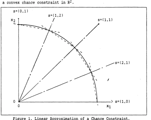
Vector s corresponds to a ray from the origin. With each vector s, the evaluation of (7) gives us a point on the boundary surface of (2). We repeat the process for a set of selected rays to get a set of points on the boundary of (2). We then connect adjacent points to form hyperplanes. The hyperplanes are introduced into the problem as linear inequalities (linear constraints). These linear inequalities replace the chance constraint (1) in the problem.
Geometrically, the linear inequalities form a polyhedron that has extreme points touching the boundary of the feasible region. Consequently, if the feasible region formed by (2) is convex, it "contains" the
polyhedron. Therefore when (2) is convex, the set of linear inequalities is uniformly tighter than (2). The extreme points are the same points at which
region. Figure 1 illustrates the polyhedron formed by the extreme points in a convex chance constraint in R2.
Figure 1. Linear Approximation of a Chance Constraint.
With an infinite number of rays, the linear inequalities reproduce the chance constraint (1). In practice, only a few "well-chosen" rays are
needed to give solutions with small relative errors from the optimal value. EXAMPLES
All our linear approximations have the form
Eni=l Qik Xi b, k=l,..,K, (8)
where 2ik, i=l,..,n, are deterministic coefficients. For each k, Eni=l Qik Xi = b defines a hyperplane and -Qik, i=l,..,n, are obtained by solving a system of equations; each equation corresponds to an extreme point (of the polyhedron) that rests on the hyperplane. This effort is done once only for each approximation; they are not solved each time the approximation is used. (Details are presented in the appendix.)
11 s=(0,1) s=(1,2) X2 -s=(2,1) s=(1,0) 0 1 X1 I
In this study we provide, as examples of the general approach, three approximations: (RAY1). (RAY2), (RAY3). The rays used in these
approximations are the decision variable axes and the centriod rays, rays in the center of the cone formed by subsets of the axes. Allen, Braswell, and Rao [1974] and Olson and Swenseth's [19871 methods are special cases of
(RAY1); the rays used in (RAY1) are the decision variable axes only.
We define the unit vector ei = (sl,..,sn )where sj = 1 for i = i and sj = 0 otherwise. Below, we provide the approximations.
(RAY1)
(RAY2)
For n = 3, for example, matrix Q = [Qik]
(1,1,1)-(0,1,0)-(0,0,1) (0 (0,1,0) ,0,1)
= (1,0,0) 0(1,1,1)-0(1,0,0)-(0,0,1) ,(0,0,1)
(1,0,0) (0,1,0) 0(1,1,1)-0(1,0,0)-(0,1,0)
For (RAY3), we construct unique sets {t(i,k), i=l,..,n), k=l,..,K. By itself, each n(i,k) is also a set such that (i-l,k) c n(i, k),
i=l,..,n, with (n,k) = {1,..,n) and (O,k) = {} for all k. Note that there can be n! unique sets of {t(i,k), i=l,..,n} and hence K = n!.
gRAY1x( )i = ni=l ik Xi, k=l,..,K=l,
where ik = (ei), k=l,..,K=l.
gRAY2(x) = ni=l ik Xi, k=l,..,K=n,
where Qik = (Enj=1 ej) - Enj=1 (ej) + (ei ) for i = k
and ik = (ei) otherwise.
(RAY3)
gRAY3(x) = Eni=l ik Xi, k=l,..,K=n!,
where Qik = (Eren(j,k) Sr) - O(ret(j-l,k) Sr)
with j such that i = (ji,k)\n(j-l,k). (\ is the set subtraction operation.)
Now for n = 3, 4(1,,1)-4(0,1,1) (0,1,1)-(0,0,1) 4(0,0,1) 0(1,1,1)-4(0,1,1) C(0,1,0) 4(0,1,1)-(0,1,0) O(1,0,1)-%(0,0,1) O(1,1,1)-(1,0,1) ~(0,0,1) (,,0(1101) ~(1,,1)-0(1, 0,0) (1,1,0)-4(0,1,0) 4(0,1,0) 4(1,1,1)-4(1,1,0) 4(1,0,0) 41,1,0)-(1,0,0) O(l,1,1)-C(1,,0)
(RAY1), (RAY2), and (RAY3) are by no means the only approximations possible using our methodology. There can be numerous variations by using different rays and constructing different hyperplanes from them. Moreover, an iterative multi-pass approach may be devised to generate the rays based on previous iterations solution. We leave this challenge for future
research. FRACTILES
When the joint probability distribution of the random variables are known, the fractiles (s) may sometimes be obtained as closed-form
expressions. Alternatively, at a level of confidence that corresponds to their sample sizes, the fractiles can be extracted from Monte-Carlo
simulation (Levy [1967]) or sample data. If the form of the distribution is known but not the exact distribution, the fractiles may be estimated using statistical approximation methods (Bache [1979], Cornish and Fisher [1937], Fisher and Cornish [1960]). These methods can make use of the sampling
13
information beyond the first two moments. When the sample data only is available, distribution-free or non-parametric methods (Allen, Braswell, and Rao [1974], Wilks [1963]) may be used.
4. Comparative Experiments
We compare our method against those by Hillier, Seppala, and Olson and Swenseth. Before proceeding, we sketch how these methods approximate g(x) for the test conditions we are using. Following that, we describe the test conditions and then state the comparison criterion.
g(x) _ F (Eni=l a1 i xi; a)
Normal distribution:
g(x) = ni=1 E[ai] Xi + Za [Eni=1 i2 xi2 11/2.
Uniform distribution and xi e 0,1, i=l,..,n:
g(x) = m - (m!(1-a))1/m where m = Eni=1 xi.
For xi e 0,11, g(x) for the uniform distribution case can be derived using geometry.
(HILL)--Hillier
(a/(l-a))1/ 2 is the one-sided Chebyshev's inequality safety factor.
Approximation gHILL(x) given above is only the nonlinear approximation of Normal distribution and xi e [0,1], i=l,..,n:
gHILL(X) = Eni=1 E[ai] Xi + Za [Eni=1 (02 - oi2 + oi2 xi2)"/2 - (n-1)e]
Uniform distribution and xi e (0,1, i=l,..,n:
gHILL(X) = Eni=lE[ai] xi + (a/(1-a))1 / 2 [Eni=1 ( - (e2 - ai2)1/2) xi
+ Eni=1 (2 - ai2)1/2 - (n-1)6]
where e = (Eni=1 ci2)1/2.
--Hillier's method. For the comparison tests, we did not linearize it. The reader will realize that, for our comparison criterion, the result using gHILL(x) will be an upper bound on the linearized version.
(SPLK)--Seppdla
Normal distribution and xi > 0, i=l,..,n:
gSPLK(X) = Eni= l E[ai] xi + Za Yn
where Yi = Max {rik Yi-1 + ik xi, k=1,..,K} with y = 0,
tik (1 + i2 ti,k1 2)1/2 - ti,k-l (1 + i2 tik2 )/2
rik
=---ti - ti,k-l1
(1 + i2 ti,k2)1/2 - (1 + oi2 ti,k-12)l/2 Sik =
ti - ti,k-l1
and tik = TANGENT[(k/K)(n/2)3/i1 /2, i=l,..,n, k=l,..,K.
Uniform distribution and xi 0, i=l,..,n:
Same as above except replace Za by (a/(1-a))1/2.
We consider the instances where K = 3 and 6 which we label (SPL3) and (SPL6) respectively. Seppala's approach replaces each chance constraint with O(nK) linear inequalities.
(OLSW)--Olson and Swenseth
Normal distribution and xi 0, i=l,..,n:
gOLSW(x) = Eni=1 (ECai] + Za ai) xi.
Uniform distribution and xi 0, i=l,..,n:
gOLSW(x) = ni=1 (E[ai ] + (a/(1-a))1/2 i) Xi.
(OLSW) is the same as (RAY1) under condition C1 and if z is available. (RAY1, RAY2, and RAY3)
The approach we propose in this study leads to a class of approximations. For the purpose of comparison, we use only (RAY1), (RAY2), and (RAY3).
III
Under the normal distribution, (s) = i=1 E[ai] i + Za [ni=1 i2 si211/2; and for the uniform distribution case with i e {0,11, (s) = m
-(m!(1-a))l/m where m = Eni=1 Si. With the expression for ¢(s) given, approximations (RAY1), (RAY2), and (RAY3) are completely defined.
For simplicity of conducting the experiments, we test only cases where the random variables are independent identically distributed. (All
the methods tested can be used for dependent and non-identically
distributed random variables. In the future, we hope to perform extensive experiments on these cases and report our findings.) First, we evaluate cases where ai, i=l,..,n, are normally distributed with xi [0,1],
i=l,..,n. Here, we examine how well our methods compare against the other methods in the conditions specified for those methods. Since the conditions are those that the other methods were derived under, we can expect our methods to do no better than these methods. Then we compare the methods when ai, i=l,..,n, are uniformly distributed with xi e (0,1}, i=l,..,n. Here, we test for the situation of a non-stable distribution for which the exact analytical form of g(x) is known. We would expect the other methods to do poorly under non-stable distributions since they were intended for such conditions and have to use the Chebyshev's inequality.
In general, the conditions are specified to keep the tests simple or to replicate the conditions that were originally intended for the other methods. The test input data are generated as follows:
(a) For the normal distribution cases, we let E[ai = 0.5, i=l,..,n, and
pick variance i2 = 2, i=l,..,n, from a uniform distribution in [O0,VA]. We
examine cases where VA = 10-B, B = 0,..,4. The maximum coefficient of variation (COV), in each case of B, is VA/0.5. Overall, the COV ranges from 0 to 2. The values of decision variables xi, i=l,..,n, are sampled
from a uniform distribution in [0,1]. We tested cases where n = 2, 4, and 6.
(b) For the uniform distribution cases, we sample ai, i=l,..,n, from a
uniform distribution in [0,1]. Hence, E[ail = 0.5, i= l,..,n, and variance oi2 = 2 = 1/412 and COV (1/412)/0.5 = 0.58. To obtain xi {0,1}, we
sample from a uniform distribution in [0,13. We then let xi = 0 when the
sampled value is less than 0.5; and xi = 1 otherwise. We evaluated the cases where n = 2, 4, 6, 8, 16, and 32.
The criteria of comparison is the relative error that the values of the approximation deviate from g(x): relative error of method h - (gh(x)-g(x))/g(x). Since all the methods to be compared are uniformly tighter than (1), g(x) < gh(X) < b, h {HILL, SPL3, SPL6, OLSW, RAY1, RAY2, RAY3}. Therefore, the relative error is non-negative; it is a measure of how
constricted approximation h is when (1) is binding and the sampled value of x is the optimum solution. We replicated each set of test conditions 15
tipes and compute their average and standard deviation.
5. Results and Comments
First, we note that our three approximations have different
computation requirements. (RAY1) replaces each chance constraint with one linear inequality; (RAY2) uses n linear inequalities and (RAY3) uses n! linear inequalities. (RAY1) and (RAY3) represent examples of the extreme types of our class of approximations. (RAY3), especially, will be difficult to implement for n larger than 6; it took about 50 seconds to evaluate one chance-constrained approximation on a IBM-PC compatible 80286 class machine when n = 6. (RAY1), (RAY2), and other methods took a negligible amount of time--typically less than 1 second per evaluation of g(x). Second, the result of (RAY3) dominates that of (RAY2) and the result of (RAY2)
dominates that of (RAY1). This is because (RAY3) is uniformly tighter than (RAY2) and (RAY2) is uniformly tighter than (RAY1). We can therefore use the results of one approximation as a bound to another.
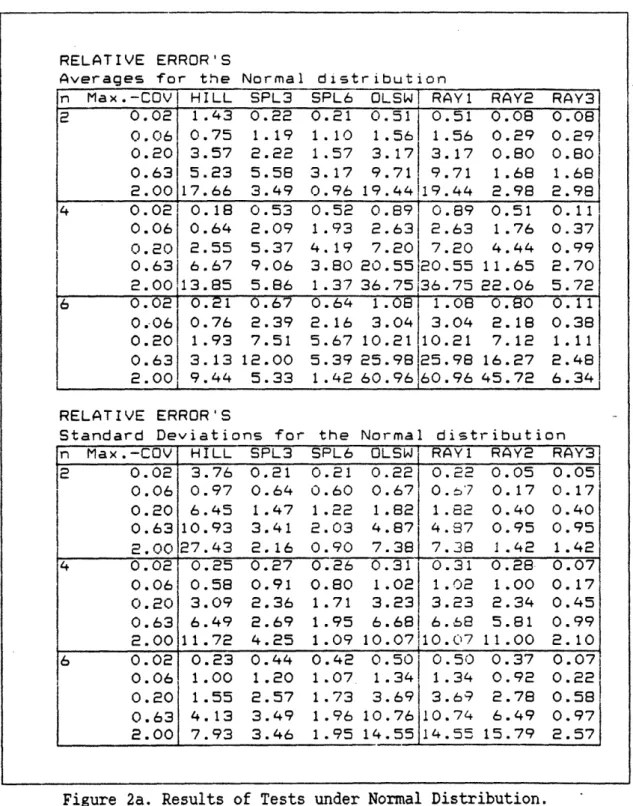
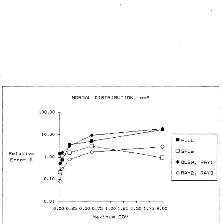
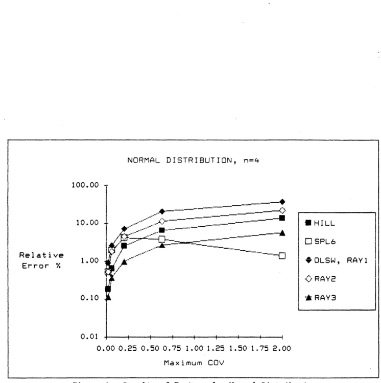
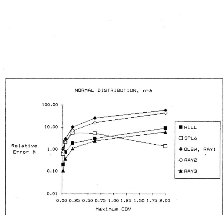
The comparisons outcome is tabulated in figures 2a through 3b. Figure 2a tabulates the average and standard deviation of the relative errors for the normal distribution cases. These results are graphed in figures 2b through 2d, for n = 2, 4, and 6 respectively. For maximum-COV less than 0.5, (RAY2) does as well as (HILL) and (SPL6), but it gets progressively worse as n becomes larger. The average relative errors in such cases are about 5% or less. Since (SPL6) uses 6 times more constraints than (RAY2) and (HILL) is only the nonlinear approximation part of Hillier's method, the comparable results among the three methods suggest that our methods perform well for small n.
[INSERT FIGURES 2a THROUGH 2d HERE]
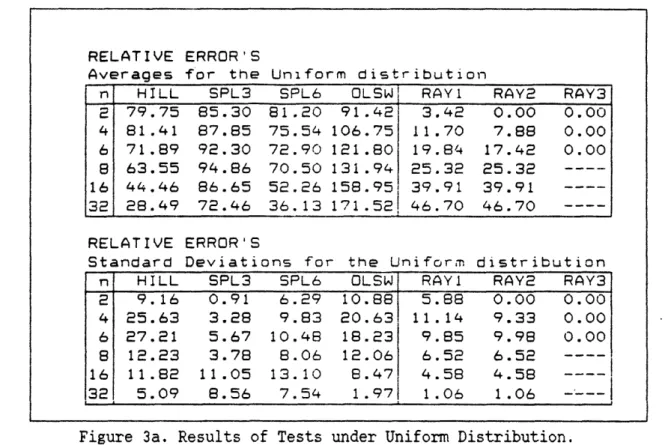
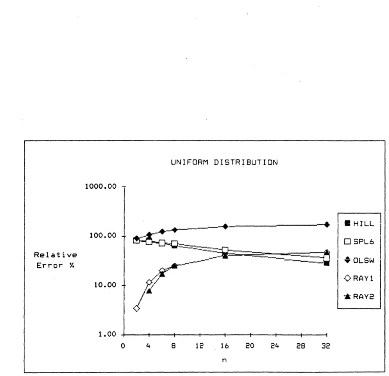
For the uniform distribution cases, figure 3a tabulates the results while figure 3b presents it graphically. In these cases for n up to 6,
(RAY3) is exact. We did not test (RAY3) beyond n = 6 since the computation effort is too much. (RAY1) and (RAY2) performed equally well and are about an order of magnitude better than (HILL) and (SPL6) when n is less than 6. They dominate the other methods up to n = 16. The methods, except for
(OLSW), have about the same size of errors when n is larger than 16. (OLSW), on the whole, demonstrated to be an inferior method.
[INSERT FIGURES 3a AND 3b HERE]
The results of both the normal and uniform distribution cases show that the average relative errors become worse with larger n. As such, we do not recommend using any of the methods, ours included, for COV's larger than 0.5 when n gets beyond 12; the average relative errors then goes up to more than 50%. As mentioned in the introduction of this paper, large n may be permitted in production/inventory problems because of its block
triangular structure. When the planning is done on a rolling horizon basis, the large errors for the periods further away are not important as long as the nearer periods are well approximated. This is the case when a method like (RAY2) is applied. In fact, (RAY1), (RAY2), and (RAY3) are exact for n
1, the first period problem.
The number of random coefficient, n, may also be large when the capacity constraints limit the number of non-zero decision variables, of those in the chance constraint. (An example of this is where there are many alternative processes of producing a product and only a few are permitted.) In these cases, the "effective" number of random coefficients in the chance constraint will be small. Again, (RAY2) should perform very well there. EXTENSIONS AND FU _RE RESEARCH
We have assumed zero-order decision rules (see Charnes and Cooper [1963); all the decision variables to be determined before the value of any random variables are known. The linear formulation of our method can be adapted easily to give solutions for linear decision rules. A linear
decision rule for a decision variable is a linear combination of the random variables that will be realized before that the decision variable needs to be determined. Therefore for problems with sufficient stationarity, we can solve the problem once, replacing all decision variables by the decision rules, to obtain the parameters for the decision rules. As the value of
19
---random variables become known, we apply the decision rules to get the values of the decision variables, without resolving the linear program.
The chance constraints we have examined are for linear inequalities--that is, the term inside of Prob(.) in (1) is a linear function. Our
approach does not restrict us to linear inequalities; we can have nonlinear inequalities or situations where ai = ai(x), i=l,..,n, are functions of x. In production problems with stochastic yield, the last situation
corresponds to the case where the yields are not independent of the lot size; a problem that has chance constraint like constraint (1) corresponds to the case where the yields are independent of the lot size.
For future research, we suggest to consider the following: (a) examine how the relative errors can be parametrically bounded, (b) provide a multi-pass e-optimal iterative approach, (c) consider problems with joint chance constraints, (d) provide theoretical results on the convexity of the feasible region.
6. Summary and Conclusions
We provided a class of linear approximations for problems with individual chance constraints that have random variables with arbitrary distributions. In our method, we linearized the nonlinear deterministic equivalents of chance constraints when the deterministic equivalents may not have closed-form expressions. The linear approximation is uniformly
tighter than the chance constraint when the feasible region defined by the latter is convex. Therefore under convexity, the solutions generated by our approximations will satisfy or do better than the service target specified by the chance constraint.
Our method gives linear inequalities that retain the original
order decision rules. The resulting programs are linear programs which permit the use of standard LP codes, perform sensitivity analysis, and have both primal and dual solutions. The coefficients in the approximating
linear constraints can be extracted from assumed distributions or sample data. We do not restrict the distributional form of the random variables, disallow their dependencies on each other or require their partial
derivatives.
The user has the option of trading-off the amount of computation effort against the accuracy of the solution by selecting the number of linear inequalities. In the simulation tests, when the number of random variables are small, applications of our approach with very few
inequalities compare very well against the existing methods for both the normal and the uniform distributions.
The authors are grateful to Steve Gilbert for his comments on an earlier version of this paper.
REFERENCES
ALBIN, S.L. and D.J. FRIEDMAN 1989. "Impact of Clustered Defect Distributions in IC Fabrication," Mgmt. Sci. 35:1066-1078. ALLEN, F.M., R. BRASWELL, and P. RAO 1974. "Distribution-free
Approximations for Chance-Constraints," Op. Res. 22:610-621.
BACHE, N. 1979. "Approximate Percentage Points for the Distribution of a Product of Independent Positive Random Variables," Appl. Statist. 28:158-162.
BITRAN, G.R., and T-Y. LEONG 1989a. "Deterministic Approximations to Co-production problems," MIT Sloan Sch. Working paper #3071-89-MS.
BITRAN, G.R., and T-Y. LEONG 1989b. "Co-production of Substitutable Products," MIT Sloan Sch. Working paper 3097-89-MS.
BITRAN, G.R., and T-Y. LEONG 1989c. "Hotel Sales and Reservations Planning," MIT Sloan Sch. Working paper #3108-89-MSA.
III
BRADLEY, HAX, and MAGNANTI 1977. Applied Mathematical Programming, Addison-Wesley Publ., Reading, Mass.
CHARNES, A., W.W. COOPER, and G.H. SYMONDS 1958. "Cost Horizons and
Certainty Equivalents: an Approach to Stochastic Programming of Heating Oil," Mgmt. Sci. 4:235-263.
CHARNES, A., and W.W. COOPER 1963. "Deterministic Equivalents for
Optimizing and Satisficing under Chance Constraints," Op. Res. 11:18-39. CHARNES, A., W.W. COOPER, and G.L. Thompson 1963. "Characterizations by
Chance-constrained Programming," in Recent Advances in Mathematical Programming, Graves, R. and P. Wolfe (editors).
CHARNES, A., M. KIRBY, and W. RAIKE 1970. "An Acceptance Region Theory for Chance-constrained Programming," J. Math. Anal. Appl. 32:38-61.
CORNISH, E.A. and R.A. FISHER 1937. "Moments and Cumulants in the Specification of Distributions," Rev. Int. Statist. Inst. 5:307-321. DEMPSTER, M.A.H. 1980. Stochastic Programming, (Dempster ed.), Academic
Press, New York.
FISHER, R.A. and E.A. CORNISH 1960. "The Percentile Points of Distributions having Known Cumulants," Technometrics 2:209-225.
HOGAN, A.J., J.G. MORRIS, and H.E. THOMPSON 1981. "Decision Problems under Risk and Chance-Constrained Programming: Dilemmas in the Transition," Mgmt. Sci. 27:698-716.
HILLIER, F.S. 1967. "Chance-Constrained Programming with 0-1 or Bounded Continuous Decision Variables," Mgmt. Sci. 1:34-57.
KALL, P. 1976. Stochastic Linear Programming, Springer-Verlag, New York. KATAOKA, S. 1963. "A Stochastic Programming Model," Econometrica
31:181-196.
KELLY, J.E. 1960. "The Cutting Plane Method for Solving Convex Programs," SIAM Jour. 8:703-712.
LEVY, L.L. and A.H. MOORE 1967. "A Monte-Carlo Technique for obtaining System Reliability Confidence Limits from Component Test Data," IEEE trans. Rel. R-16:69-72.
OLSON, D.L. and S.R. SWENSETH 1988. "A Linear Approximation for Chance-Constrained Programming," J. Opl. Res. Soc. 38:261-267.
PREKOPA, A. 1971. "Logarithmic Concave Measures with Applications to Stochastic Programming," Acta Sci. Math. (Szeged) 32:301-316.
PREKOPA, A. 1974. "Progranming under Probabilistic Constraints with a Random Technology Matrix," Math. Operationsforsh. Statist. 5:109-116.
PREKOPA, A. 1988. "Numerical Solution of Probabilistic Constrained Programming Problems," in Numerical Techniques for Stochastic
Optimization (Y. Ermoliev and R. J-B. Wets eds.), Springer-Verlag, New York.
SENGUPTA, J.K. 1972. Stochastic Programming--Methods and Applications, North-Holland.
SEPPALA, Y. 1971. "Constructing Sets of Uniformly Tighter Linear approximations for a Chance Constraint," Mgmt. Sci. 17:736-749.
SEPPALA, Y. 1972. "A Chance-Constrained Programming Algorithm," BIT 12:376-399.
SYMONDS, G.H. 1967. "Deterministic Solutions for a Class of Chance-Constrained Programming Problems," Op. Res. 15:495-512.
VADJA, S. 1972. Probabilistic Programming, Academic Press, New York. VAN DE PANNE, C. and W. POPP 1963. "Minimum Cost Cattle Feed under
Probabilistic Protein Constraints," Mgmt. Sci. 9:405-430. WILKS, S.S. 1963. Mathematical Statistics, John Wiley, New York.
APPENDIX
Probability of the event argument. Expectation function.
Variance function.
Cumulative density function of any random variable u evaluated at v, and F-l(u;.) is its inverse function.
Number of decision variables in the chance constraint.
Random technology coefficients with finite mean E[ai] and finite variance oi2, i=l,..,n.
Resource parameter.
Decision variables, i=l,..,n.
Service performance target; probability target for satisfying.the chance constraint. (Typically, a e [0,11 is close to 1.)
(S1,..,s n ) = F-1(Eni=l ai i; a) where i > 0, i=l,..,n.
Safety factor with service target a.
Safety factor for normal distributions: one-tail normal variate for a. NoQtation. Prob(.): E[.]: F(u;v): F(u;v): b: xi: a:
Sstm_ fEations t solve to obtain matrix F _ ik]
Prob(Eni=l ai xi ni=1 Qik xi, k=l,..,K) > a (al)
and En i= Qik Xi < b, k=l,..,K (a2)
=> Prob(ni=l ai Xi < b) a. (a3)
Since (a2) replaces chance constraint (a3) in the linear program
approximation, to approximate (a3) we need only focus on (al). We determine Pik, i=l,..,n and k=t,..,K by solving a system of equations, one for each
k.
Note that in inequality (al), the absolute value of vector x is not important; we need only to know the relative values among its components xi, i=l,..,n. ni=1 ik Xi = b, k=l,..,K, are a set of hyperplanes. We let
{Slk,...,SnkI be the set of rays such that hyperplane k, k=l,..,K, is
formed by the points at which these rays intersect the boundary of (a3). Each Sik, i=l,..,n and k=l,..,K, is a vector of dimension n.
The extreme points of the polyhedron that form hyperplane k,
k=l,..,K, correspond to the fractiles (Sik), i=l,..,n. (Recall that for any vector (sl,..,sn), (sl,..,sn ) = F-1(Eni=l ai i; a), i=l,..,n.) Therefore, Prob(Eni=l ai wi Eni=1 Qik wi) 2 > for all w _ (wl,..,wn) =
Enj=1 j Sik, k=l,..,K, where Enj=1 ,j = 1 and 0 ! pj < 1, j=l,..,n.
Hence, the system of equation to solve to obtain is
Slk _Qk -(Slk)
· = : , k=l, .. ,K. (a4)
L
Snk nk _ (Snk)For n=3, we present the following examples:
o1 = [2(1 1
1)
O O 1 [( 3] O 1) 1 O O Q12 (1 0) 1 1 1 Q22 (1 1 1) O O 1 (0 (32 0 1) 1 0 Q13 ¢(1 0 0) 0 1 0 23 = (0 1 0) ~ [ I ooi 1 1 Q33 (1 1 1) 1 1 Q1 (1 1 1) 1 0 0 14 (100)O 1 1 Q21 =
(o1 1)
0
1 1 1
24 =
1 1 1)
O O 1 Q3 lj 00 1) . 1 0 1 3J L(1 1) 11 1 1[012 ( 1 1) 11 FQ151 ( 1 0) o 1 o2
(O
1 0) o 1 (O 1 0) o 11 =2 (o 1 1) 1 1 2 o l(1 1 1)o
131
3
(1 0 1)
011
1
0[(1 O0)
1 1 1 IQ231 = 4 (1 1 1) 1 1 0 26 = (1 1 0) 0 0 1 33 0 1) 0 0 1 Q36 0 1)J IIIRELATIVE ERROR'S
Averages for the Normal distribution
n Max.-COV HILL SPL3 SPL6 OLSWI RAY1 RAY2 RAY3 2 0.02 1.43 0.22 0.21 0.51 0.51 0.08 0.08 0.06 0.75 1.19 1.10 1.561 1.56 0.29 0.29 0.20 3.57 2.22 1.57 3.17 3.17 0.80 0.80 0.63 5.23 5.58 3.17 9.71 9.71 1.68 1.68 2.00 17.66 3.49 0.96 19.44119.44 2.98 2.98 0.02k 0.18 0.53 0.52 0.89 0.89 0.51 0.11 0.06 0.64 2.09 1.93 2.631 2.63 1.76 0.37 0.20 2.55 5.37 4.19 7.201 7.20 4.44 0.99 0.63 6.67 9.06 3.80 20.55t20.55 11.65 2.70 2.00 13.85 5.86 1.37 36.75136.75 22.06 5.72 6 0.021 0.21 0.67 0.64 1.08 1.08 0.80 0.80 0.11 0.-06 0.76 2.39 2.16 3.04 3.04 2.18 0.38 0.20 1.93 7.51 5.67 10.21 10.21 7.12 1.11 0.63 3.13 12.00 5.39 25.98 25.98 16.27 2.48 2.001 9.44 5.33 1.42 60.96 60.96 45.72 6.34 RELATIVE ERROR'S
Standard Deviations for the Normal distribution n Max.-COV HILL SPL3 SPL6 OLSW! RAY1 RAY2 RAY31 2 0.02 3.76 0.21 0.21 0.22 0.22 0.05 0.05! 0.06 0.97 0.64 0.60 0.67 0.7 0.17 0.17 0.20 6.45 1.47 1.22 1.82 1.82 0.40 0.40 0.63 10.93 3.41 2.03 4.87 4.97 0.95 0.95 2.00 27.43 2.16 0.90 7.38 7.38 1.42 1.42 4 0.02 0.25 0.27 0.26 0.311 0.31 0.28 0.07 0.06 0.58 0.91 0.80 1.02 1.02 1.00 0.17 0.20 3.09 2.36 1.71 3.23 3.23 2.34 0.45 0.63 6.49 2.69 1.95 6.68 6.68 5.81 0.99 2.00 11.72 4.25 1.09 10.071 10.07 11.00 2.10 6 0.02 0.23 0.44 0.42 0.501 0.50 0.37 0.07 0.06, 1.00 1.20 1.07 1.341 1.34 0.92 0.22 0.20 1.55 2.57 1.73 3.69 3.69? 2.78 0.581 0.63 4.13 3.49 1.96 10.76 10.74 6.49 0.97 2.00 7.93 3.46 1.95 14.55 14.55 15.79 2.57
Figure 2a. Results of Tests under Normal Distribution.
1.00 NORMAL DISTRIBUTION, n=2 /%/% /%/% I VV. VV 0 _. __-- 4 ---0--- --- -__ Fs Relative Error % 0.10 0.01 0.00 0.25 0.50 0.75 1.00 1.25 1.50 1.75 2.00 Maximum COV
Figure 2b. Results of Tests under Normal Distribution.
E HILL { SPL6 · OLSW, RAY1 ,>RAY2, RAY3 I I" I I l I I I 10.00
NORMAL DISTRIBUTION, n=4 I VV VV -10.00 Relative Error % 1.00 I 0.10 0.01 0 ...-- _ A ..-- , . ..,. _____ b --- _ -- i=~~~~-.00 0.25 0.50 0.75 1i=~~~~-.00 1.25 1.50 1.75 2i=~~~~-.00 Maximum COV
Figure 2c. Results of Tests under Normal Distribution.
29 A HILL O" SPL6 *OLSW, RAY1 V" R AY2 - RAY3 !. . , I I * I ! --- -- ^-111---111.--- --_.. _ NFr urn
-NORMAL DISTRIBUTION, n=6
Figure 2d. Results of Tests under Normal Distribution.
30 1 VV. ·VV 10.00 Relative Error % 1.00 0.10 0.01 0.00 0.25 0.50 0.75 1.00 1.25 1.50 1.75 2.00 Maximum COV I HILL D, SPL6 *OLSW, RAY1 <> RAY2 -A RAY3 _ _ h hrr
RELATIVE ERROR'S
Averages for the Uniform distribution
n HILL SPL3 SPL6 OLSW! RAY1 RAY2 RAY3
2 79.75 85.30 81.20 91.42 3.42 0.00 0.00 4 81.41 87.85 75.54 106.75 11.70 7.88 0.00 6 71.89 92.30 72.90 121.80 19.84 17.42 0.00 8 63.55 94.86 70.50 131.94 25.32 25.32 16 44.46 86.65 52.26 158.953 39.91 39.91 32 28.49 72.46 36.13 171.52! 46.70 46.70 ----RELATIVE ERROR'S
Standard Deviations for the Uniform distribution
n HILL SPL3 SPL6 OLSW RAY1 RAY2 RAY3 2 9.16 0.91 6.29 10.88 5.88 0.00 0.00 4 25.63 3.28 9.83 20.63 11.14 9.33 0.00 6 27.21 5.67 10.48 18.23 9.85 9.98 0.00 8 12.23 3.78 8.06 12.06 6.52 6.52 16 11.82 11.05 13.10 8.47 4.58 4.58 ----32 5.09 8.56 7.54 1.97 1.06 1.06
Figure 3a. Results of Tests under Uniform Distribution.
31
UNIFORM DISTRIBUTION Relative Error % 100.00 . 1000.00 I HILL C SPL6 OLSW RAY1 -* RAY2 ----., _-t/:~Y 1.00 0 4 8 12 16 20 24 28 32 n
Figure 3b. Results of Tests under Uniform Distribution. 10.00 v III .