Short wave phase shifts by large free surface solitary waves. Experiments and models

HAL Id: hal-00182831

https://hal.archives-ouvertes.fr/hal-00182831

Submitted on 5 Feb 2020

HAL is a multi-disciplinary open access

archive for the deposit and dissemination of

sci-entific research documents, whether they are

pub-lished or not. The documents may come from

teaching and research institutions in France or

abroad, or from public or private research centers.

L’archive ouverte pluridisciplinaire HAL, est

destinée au dépôt et à la diffusion de documents

scientifiques de niveau recherche, publiés ou non,

émanant des établissements d’enseignement et de

recherche français ou étrangers, des laboratoires

publics ou privés.

Distributed under a Creative Commons Attribution| 4.0 International License

Short wave phase shifts by large free surface solitary

waves. Experiments and models

Katell Guizien, Eric Barthélemy

To cite this version:

Katell Guizien, Eric Barthélemy. Short wave phase shifts by large free surface solitary waves.

Ex-periments and models. Physics of Fluids, American Institute of Physics, 2001, 13 (12), pp.3624-3635.

�10.1063/1.1409964�. �hal-00182831�

Short wave phase shifts by large free surface solitary waves: Experiments

and models

Katell Guiziena) and Eric Barthe´lemy

Laboratoire des Ecoulements Ge´ophysiques et Industriels, BP 53, 38041 Grenoble Cedex 9, France 共Received 2 May 2000; accepted 17 July 2001兲

In this paper, we compare experiments on short gravity wave phase shifting by surface solitary waves to a Wentzel–Kramers–Brillouin–Jeffreys共WKBJ兲 refraction theory. Both weak interactions

共head-on interaction兲 and strong interactions 共overtaking interaction兲 are examined. We derive a

dispersion relation and wave action conservation relation which are similar to the ones obtained for short waves refraction on slowly varying media. The model requires an exact solitary wave solution. To this end, a steady wave solution is numerically computed using the algorithm devised by Byatt-Smith 关Proc. R. Soc. London, Ser. A 315, 405 共1970兲兴. However, two other solitary wave solutions are incorporated in the model, namely the classical Korteweg and De Vries共KdV兲 关Phil. Mag. 39, 422共1895兲兴 solution 共weakly nonlinear/small amplitude solitary wave兲 and the Rayleigh

关Phil. Mag. 1, 257 共1876兲兴 solution 共strongly nonlinear/large amplitude solitary wave兲.

Measurements of the short wave phase shift show better agreement with the theoretical predictions based on the Byatt-Smith numerical solution and the Rayleigh solution rather than the Korteweg and De Vries one for large amplitude solitary waves. Theoretical phase shifts predictions based on Rayleigh and Byatt-Smith numerical solutions agree with the experiments for A/h0⭐0.5. A new heuristic formula for the phase shift allowing for large amplitude solitary waves is proposed as a limiting case when the short wave wave number increases. © 2001 American Institute of Physics.

关DOI: 10.1063/1.1409964兴

I. INTRODUCTION

In the present paper we analyze how short surface waves are modulated by free surface solitary waves. This approach may be considered as a model of a more complex interaction problem, namely nonlinear internal wave–surface wave in-teraction. The latter is of importance for ocean remote sens-ing applications. Indeed, on synthetic aperture radar 共SAR兲 images of the ocean surface, signatures of long internal waves are due to Bragg wave modulations. From a theoreti-cal point of view free surface solitary wave and short wave interactions is a challenging problem. Indeed standard theo-ries for short waves do not encompass long nonlinear waves and vice versa. As a first cut one may consider two linear waves one of which is very long compared to the other. This is the approach initiated by Longuet-Higgins and Stewart.1 They analyzed the change of the form of short surface waves riding on longer ones within the framework of linearized theory for finite depths. Interaction terms are derived from the second order of Stokes’ theory, which requires the as-sumption of small steepness for both long and short waves. They show that the short wave has a shorter wave length and increased amplitude at the long wave’s crest. This Doppler effect is interpreted as the work done by the long wave against the radiation stress of the short one. In the same paper, the authors suggest to generalize the wave action

con-servation and the dispersion relation valid for surface waves refracted by a steady current to the case of surface waves riding upon a much longer wave 共Sec. IV兲. This implies to introduce an effective gravity resulting from the vertical ac-celerations of the long wave. Longuet-Higgins and Stewart1 then show that this latter approach yields the same result as their calculations within the second-order Stokes theory as long as the vertical accelerations of the longer wave is neg-ligible, like in shallow water共Sec. V兲. In a companion paper, Longuet-Higgins and Stewart2 made a further step forward. They analyzed the change in amplitude of a short surface wave on a steady nonuniform current. Under the slowly spa-tially varying current assumption they derive the laws ruling wave amplitude, namely wave action conservation, and wave length modulations.

The linear behavior of the long wave was relaxed by Garrett3 and later, Bretherton and Garrett4 who generalized the results obtained by Longuet-Higgins and Stewart.2 In a very general setting, using the averaged Lagrangian formu-lation, they show that the wave action conservation is a very general result for short linear wave of small steepness as long as they propagate on a spatially and temporally slowly vary-ing basic state. As just mentioned, the flow characteristics of the basic state do not need to be linear and effective gravity is introduced accounting for vertical accelerations in the underlying basic state. This is highlighted by Longuet-Higgins.5 He applied wave action conservation to show that when the long wave is steep, up to the Stokes wave maximum steepness of 0.4432, the steepness of the short wave riding on it undergoes much more enhancement

a兲_{Present address: Observatoire d’Oce´anologie Biologique, BP 44, 66650}

Banyuls-sur-Ner, France. Telephone:⫹33 4 76 82 51 17; Fax: ⫹33 4 76 82 50 01. Electronic mail: guizien@hmg.inpg.fr

3624

than would be predicted by the second-order of Stokes’ lin-ear theory developed in his 1960 paper. Longuet-Higgins also underlined the need for a very accurate description of the long wave, which he did through a particularly efficient algorithm.

The paper of Bretherton and Garrett4 is an encourage-ment to make alternative choices on the basic state. Naciri and Mei6 derived analytically the solution for a short wave riding on a long wave given by the explicit formula for Ger-stner’s rotational wave. They qualitatively reproduce Longuet-Higgins’ numerical results, and show that instabili-ties can appear for sufficiently large short wave steepness compared to the long to short wave frequency ratio.

The choice of a solitary wave has been made by a few authors and is the one made in this study. Using a method-ology similar to the one proposed by Zhang and Melville7for infinite depth, Shen et al.8 derive a nonlinear Schro¨dinger equation and wave action conservation for short waves riding on a solitary wave. This confirms the suggestion by Bretherton and Garrett.4They explicitly assume the perturb-ing wave to be a short deep water wave. They also retrieve a ‘‘wave crest’’ conservation equation. Wave number, wave amplitude, and frequency modulations of the short wave are thus computed along a solitary wave profile. The latter is computed by Evans and Ford’s9 procedure. Wave number modulations along the solitary wave is an important step towards phase shift computations. Using a WKBJ perturba-tion method within the shallow water theory, Clamond and Germain10 allowed for solitary waves of the KdV type to coexist with short waves. Predicted short wave phase shifts are shown to agree with those measured during earlier ex-periments on interactions between a short monochromatic surface wave and an external solitary wave in shallow water

共mean depth h0 of 25.5 cm兲 by Clamond and Barthe´lemy. 11

Indeed, Clamond and Barthe´lemy11 experimented two short waves frequencies of 1.5 and 2.3 Hz共k_⬁h₀ of 2.35 and 5.42 where k_⬁ is the short wave wave number兲. They only considered the case of waves propagating in opposite direc-tion 共head-on interaction兲, referred to as a weak interaction. This terminology was first introduced by Miles12for solitary wave interactions. In contrast the case of a solitary wave propagating in the same direction 共overtaking interaction兲 is called a strong interaction. It was shown that the surface wave train, after interaction, was phase-shifted compared to the surface wave train before. Phase shifts in this context had never been mentioned before in the literature. Previous theo-ries or experiments on phase shift predictions dealt with sinusoidal waves.

Longuet-Higgins and Phillips13 showed that when two sinusoidal waves of very different wave numbers interact, the phase velocity of the shorter one will be decreased or increased共depending on the relative direction of propagation of the waves兲 by an amount proportional to the mass trans-port at the surface of the longer wave. Mass transtrans-port in solitary waves produces a small but finite displacement L of the water particles. Thus, on the same ground as Longuet-Higgins and Phillips,13 it is expected that short waves inter-acting with solitary waves will be phase shifted by the dis-placement. Assuming linear superposition of motion and

instantaneous displacement, the phase shift⌬␸undergone by the short wave is expressed by

⌬␸⫽2␲_{␭ ⫽}L k_⬁L, 共1兲

where ␭ is the short-wave wave length. This heuristic for-mula depends on the expression of L⫽L(A,h0) where A is the solitary wave amplitude and h0 is the depth of water at

rest. In the present paper we discuss the relevancy of the instantaneous interaction assumption underlying 共1兲.

Experimentally, the phase shift undergone by the short wave is measured using an harmonic analysis technique. The order of magnitude of the phase shift corresponds to a short wave time shift of 0.1 second. Determination of such a small phase shift is very sensitive to a variety of perturbing phe-nomena. In Clamond and Barthe´lemy’s experiments, solitary waves had strong dispersive tails trailing the main pulse that authors claim to affect the determination of the phase shift. We improved the solitary wave generation procedure in order to minimize the undesired trailing waves. Moreover, other perturbing causes are examined.

Hereinafter, we present in Sec. II A a derivation of the wave action conservation and a new dispersion relation for first-order Stokes waves interacting with a solitary wave us-ing a WKBJ perturbation method in the rectilinear coordi-nates. This approach is similar to Shen et al.,8except that we allow for intermediate water depth and the wave crest con-servation equation is simplified in order to obtain an alge-braic dispersion relation. The solitary wave may be described either by the analytical solutions of Rayleigh14 or KdV15or by Byatt-Smith’s16 numerical solution. Assuming a KdV solitary wave, Clamond and Germain10analytical expression of the phase shift is retrieved. We discuss in Sec. II B the relevance of these different solitary wave approximations in the scope of solitary wave interaction with a short wave. The theoretical results are then compared with experiments pre-sented in Sec. III which are complementary to Clamond and Barthe´lemy.11 Indeed, for the first time, strong interactions have been produced. Moreover, a broader range of short wave wave numbers has been examined 共k_⬁h0 varies from

2.73 to 7.54兲. In Sec. IV, the wave number modulations de-duced from Sec. II A are tested through comparison with the measured phase shifts undergone by the short waves. In some cases, short waves breaking has been observed. Predic-tions of the maximum short wave steepness when breaking was observed are reported.

II. THEORETICAL ANALYSIS

The aim is to devise a two-dimensional 共2D兲 model to study short surface waves modulations when the short waves ride on a solitary wave. We use a nonviscid, incompressible and homogeneous fluid with a depth at rest h0. We assume

irrotational motions, therefore, the velocity field can be de-rived from a velocity potential⌽(x,z,t) and␩s(x,t) denotes free surface displacement with respect to the rest level.

The key step is to consider a long wave which is an exact stationary solution of this flow in a reference frame moving at the wave phase speed c. To this end, the new

horizontal variable X⫽x⫺ct that describes the co-moving frame is introduced. It has long been known that this prob-lem has an exact stationary solitary wave solution

共Lavrentiev17_{兲. At the present level of derivation it is not}

necessary to specify its expression and we denote the veloc-ity potential and the free surface displacement associated with this exact stationary wave by␾e(X,z) and␩e(X) 共see Fig. 1兲. Other exact solutions exist, amongst which are peri-odic solutions.

We now seek for infinitesimal disturbances of this exact solution. The free surface elevation and velocity potential are expanded as series of a small parameter ␦ of the following form:

␩s共X,t兲⫽␩e共X兲⫹␦␩共X,t兲, 共2兲

⌽共X,z,t兲⫽␾e共X,z兲⫹␦␾共X,z,t兲. 共3兲

As in the Stokes theory,␦is known to be proportional to the short wave surface slope. Assuming that the perturbation is sinusoidal in time of high-frequency␻and that its ampli-tude a is small compared to both its wavelength␭ and depth h0, the first-order then reduces to a classical set of linear

partial differential equations. The perturbation potential

␾(X,z,t) is a harmonic function and the bottom is imperme-able. The free surface displacement for the perturbation is given by ␩共X,t兲⫻G共X兲⫽i␻␾⫺共ue⫺c兲 ⳵␾ ⳵X⫺ve ⳵␾ ⳵z , 共4兲 where ue⫽␾eX, ve⫽␾ez and G(X)⫽g⫹(ue⫺c)veX

⫹vevez written on z⫽␩e(X). One recognizes G(X) to be the effective gravity introduced by Longuet-Higgins and Stewart1 and later Bretherton and Garrett.4 The effective gravity is the sum of the gravity and vertical acceleration at the free surface.

The free surface kinematic condition in addition to Ber-noulli’s relation leads to the following equation for the per-turbation velocity potential at the free surface z⫽␩e(X):

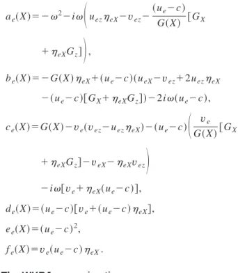
ae共X兲␾⫹be共X兲 ⳵␾ ⳵X⫹ce共X兲 ⳵␾ ⳵z ⫹de共X兲 ⳵2_␾ ⳵X⳵z ⫹ee共X兲 ⳵2_␾ ⳵X2⫹ fe共X兲 ⳵2_␾ ⳵z2⫽0, 共5兲 with ae共X兲⫽⫺␻2⫺i␻

冉

冊

be共X兲⫽⫺G共X兲␩eX⫹共ue⫺c兲共ueX⫺vez⫹2uez␩eX

⫺共ue⫺c兲关GX⫹␩eXGz兴兲⫺2i␻共ue⫺c兲, ce共X兲⫽G共X兲⫺ve共vez⫺uez␩eX兲⫺共ue⫺c兲

冉

冊

Length scales associated with the perturbation are as-sumed to be very small compared with the length scales of the long wave. The short wave is continuously adapting its characteristics to maintain itself as a high-frequency mono-chromatic wave. This assumption of WKBJ type is equiva-lent to that of Shyu and Phillips.18 A small parameter ␮

⫽␭/⌳ 共where ␭ is the short wave wavelength and ⌳ is a

characteristic length of the solitary wave兲 is naturally in-volved and a new variable X*⫽␮X is introduced. The WKBJ approximation postulates slow variations of the am-plitude A(X,z) and rapid variations in the phase S(X,z). This is written in the following form:

共6兲 ␾*共X*,z兲⫽A*_共X*,z兲e, iS*_共X*,z兲/␮,

where ␾*(X*,z)⫽␾(X,z) and A*(X*,z)⫽A(X,z) and S*(X*,z)⫽␮S(X,z) are real numbers. The amplitude and phase are expanded in even series of ␮of the form

A*共X*,z兲⫽A0*_共X*,z兲⫹␮2A2*共X*,z兲⫹¯⫹O共␮2n兲, 共7兲

S*_共X*,z兲⫽S0*_共X*,z兲⫹␮2S₂*_共X*,z兲⫹¯⫹O共␮2n兲.

共8兲

At the lowest orders 共␮⫺2 and ␮⫺1兲, the only nontrivial relation is S₀*_⫽S0*(X*). The modulated wave number k(X)⫽S_0X

*

* is then introduced.

Depending on the relative scale of␮and␦, Eq.共5兲 will simplify differently. Indeed, when ␮⬃␦ orders correspond-ing to ␮ and ␦ cannot be separated. Dingemans19 reports studies of the refraction of waves by currents for which ver-tical dependency predominates over horizontal and temporal variations by assuming ␮Ⰶ␦. Regarding the interaction problems, the correct assumption is ␮Ⰷ␦ as made by Mei20 to study the refraction of waves on slowly varying currents. The main difference here with the available literature is not to assume that the long wave is a linear one either in finite

depth or in infinite depth. Moreover, most authors have fo-cused on amplitude modification and Doppler shift. In con-trast, we will analyze the phase shift of the short wave. Our approach also differs from that of Clamond and Germain10 since they explicitly assumed a solution in the small ampli-tude approximation. In contrast, the exact solitary wave so-lution we consider can be of large amplitude. However, the coefficients of Eq. 共5兲 contain terms of different orders in

␴⫽h0/⌳, that can be sorted out. The two leading orders are given in Table I.

Assuming ␴⬃␮(␭⬃h0), the perturbation fulfills the following dispersion relation obtained by considering the or-der␮0:

⍀2_{⫽gk共X兲tanh关k共X兲共␩}

e共X兲⫹h0兲兴. 共9兲

It appears that the effective gravity reduces to gravity. The wave action conservation is retrieved at the order␮1

冋

⍀

册

with ⍀⫽␻⫺k(X)(ue(X)⫺c), a⫽A0⍀/g the short wave amplitude at the first order and Cg⫽d⍀/dk the intrinsic group velocity. The dispersion relation 共9兲 for given ue(X),

␩e(X) and c is solved numerically for k(X) using a Newton–Raphson method.

We briefly discuss qualitative behaviors. At x⫽⫾⬁ the short wave has a constant wave number k_⬁, the one ob-served in the laboratory. Note that 共9兲 differs from the dis-persion relation obtained for refraction on a slowly varying current. Indeed, changes in depth as the short wave rides on the long wave are embedded in 共9兲 since (␩e(X)⫹h0) ap-pears instead of h0 alone. The phase shift⌬␸is easily

com-puted when the modulated wave number k(X) is obtained. It reads

⌬␸⫽

冕

⫺⬁ ⫹⬁

共k共X兲⫺k⬁兲dX, 共11兲

where k(X) is the wave number in the physical space. Assuming a solitary wave solution of KdV type, the ba-sic state reads

␩e共X兲⫽⑀f共X兲h0, 共12兲

ue共X兲⫽⑀c f共X兲, 共13兲

c⫽c0共1⫹⑀/2兲, 共14兲

with ⑀⫽A/h0, f (X)⫽sech2_{(␤X/2), ␤/2⫽}

冑

0 2 ⫽gh0. We also assume that the wave number expands as a

series of⑀

k共X兲⫽k_⬁⫹⑀k1⫹O共⑀2兲. 共15兲

Expansions of the right and left-hand side of Eq.共9兲 in series of⑀including the first two leading orders yield

⍀2_{⫽共␻⫹k} ⬁c0兲2⫹⑀关2c0共␻⫹k⬁c0兲共k1⫺k⬁f兲兴 ⫹O共⑀2_{兲, 共16兲} gk tanh共k共␩e⫹h0兲兲⫽gk_⬁tanh共k_⬁h0兲 ⫹⑀关gk1tanh共k_⬁h0兲⫹gk_⬁h0共k1 ⫹k_⬁f兲共1⫺tanh2共k_⬁h0兲兲兴 ⫹O共⑀2_{兲. 共17兲}

At the lowest order, formula共9兲 together with 共16兲 and 共17兲 provides the undisturbed dispersion relation for X⫽⫾⬁

共␻⫹k⬁c0兲 2_⫽gk

⬁tanh共k⬁h0兲. 共18兲

At the next order共⑀兲, formula 共9兲 gives k1

k_⬁⫽⌫ f共X兲, 共19兲

with ⌫⫽(c0⫹␻lab/2k_⬁⫺cg)/(c0⫹cg兲 where cg

⫽d␻lab/dk_⬁ and ␻lab2 ⫽(␻⫹k_⬁c0)2. The phase shift 共11兲

then reads

⌬␸⫽⑀k_⬁⌫

冕

⫹⬁

f共X兲dX. 共20兲

We retrieve in a more general framework the phase shift

⌬␸KdVgiven by Clamond and Germain10

⌬␸KdV k_⬁h₀ ⫽ 4 )⌫

冑

We may note that ⌫ tends to 1 when the short wave frequency increases.

B. Short wave modulation for different solitary wave solutions

At this level, the exact solitary wave solution共basic state around which a perturbation is sought兲 is not specified to obtain 共9兲 and 共10兲. A different solitary wave approximation may be used, as long as the terms neglected in Eq.共5兲 using this approximation are at least an order of magnitude smaller than the perturbation contribution. This is required so that the basic flow and the perturbation can be solved separately. The numerical solution proposed by Byatt-Smith16will easily ful-fill this assumption, as the error allowed when computing it can be less than 10⫺4 on the free surface elevation whereas the short wave amplitude is of order 10⫺2. We compute Byatt-Smith numerical solution up to A/h0⫽0.7165 using the accurate and efficient algorithm devised by Byatt-Smith and Longuet-Higgins.21 The accuracy of Byatt-Smith nu-merical solution is checked against measurements of both free surface elevation and phase speed关see Figs. 2 and 3共a兲兴

TABLE I. First two orders in␮of the coefficients in共5兲 and of the effective gravity G(X). O共1兲 O共␮兲 ae(X) ⫺␻ 2 i␻vez be(X) ⫺2i␻(ue⫺c) ⫺g␩eX⫹(ue⫺c) (ueX⫺vez) ce(X) g i␻关ve⫹(ue⫺c)␩eX兴 de(X) 0 (ue⫺c) 关ve⫹(ue⫺c)␩eX兴 ee(X) (ue⫺c) 2 0 fe(X) 0 0 G(X) g 0

for A/h0⭐0.5. Indeed, we were not able to produce larger solitary wave because of the device capabilities 共see Sec. III兲.

We shall also consider analytical solutions 共which are not strictly speaking exact solutions兲 including the KdV or shallow water approximation, which rely on both long waves and small-amplitude assumptions共weakly nonlinear theory兲. Within the shallow water theory, all series expand in either even or uneven powers of ⑀⫽A/h0. This means that the order of magnitude that separates two consecutive approxi-mations is at least ⑀2. Accordingly if first-order approxima-tion is of order 1, correcapproxima-tions to obtain a second-order ap-proximation will be of order⑀2. Between 1 and⑀2, we ought to be able to solve separately the perturbation first order (⬃␦⫽ak) leading to 共9兲 and giving the rapid variation of the phase, and the second-order 共⬃␦␮兲 leading to 共10兲 and describing the slow variations in the amplitude of the pertur-bation. This means that it is necessary for ⑀2Ⰶ␮␦, which can be met in the KdV domain of validity when⑀is less than 0.15.

Avoiding the latter restriction of small amplitude, namely allowing ⑀ to be of order 1 共strongly nonlinear theory兲, Rayleigh14 derived the following solitary wave so-lution, reported by Lamb22共Sec. 252兲:

␩共x,t兲⫽A sech2_{关␤共x⫺ct兲/2兴, 共22兲} ␤ 2⫽

冑

冑

with the depth-averaged velocity given by

u

¯共x,t兲⫽c

冉

h0⫹␩共x,t兲

冊

and the horizontal and vertical velocity given by

u共x,z,t兲⫽u¯⫹共␩⫹h0兲 2 6 ¯uxx⫺ 共z⫹h0兲2 2 ¯uxx, 共26兲 v共x,z,t兲⫽⫺u¯x共h0⫹z兲. 共27兲

This is the steady solution of the set of equations pro-posed by Serre23and later by Su and Gardner24in a strongly nonlinear framework.

Since we assume ␴⬃␮ and in order to be consistent with our WKBJ perturbation method, the horizontal velocity at the free surface ue(X,␩e) will be taken equal to u¯ when truncating terms of order␮2 and higher in共5兲 for Rayleigh and KdV approximations. For Byatt-Smith exact numerical solution, since this order separation is not possible, ue(X,␩e) will be taken equal to the full free surface horizontal velocity contribution. Moreover, separating orders, we require that

␴4_{Ⰶ␮␦, which means ␦Ⰷ␴}3_{. This condition will be}

ful-filled in the experiments.

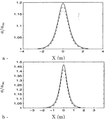
FIG. 2. Dimensionless free surface elevation at one location vs time共a兲 and in the steady reference frame共b兲 obtained for Byatt-Smith’s numerical so-lution共—兲, KdV 共- -兲, or Rayleigh’s 共¯兲 analytical solutions and experi-ments共䊊兲.

FIG. 3. Froude number F⫽c/冑gh0vs solitary wave dimensionless

ampli-tude A/h0共a兲 and outskirts decay coefficient ␤vs Froude number共b兲

ob-tained for Byatt-Smith’s numerical solution共␤is then the Stokes outskirts decay coefficient solution of the relation F2_{⫽tan(␤)/␤)共—兲, KdV 共- -兲, or}

As mentioned in the Introduction, the short wave phase shift can be deduced heuristically from the particle displace-ment L at the free surface of the solitary wave. The particle displacement L at the free surface is defined in general by

L⫽2

冕

0

⬁c⫺u共x,␩兲

u共x,␩兲 dx, 共28兲

where u(x,␩) denotes the horizontal velocity at the solitary wave free surface in the co-moving frame and c is the soli-tary wave phase speed.

In the Korteweg and De Vries15approximation, the hori-zontal velocity at the free surface is the mean horihori-zontal velocity and L is given explicitly by

L⫽ 4

)h0

冑

A h0

. 共29兲

Thus, we note that formula 共21兲 tends to the heuristic formula 共1兲 where L is given by 共29兲 for high-frequency short wave. For large amplitude solitary waves (0.4⭐A/h0

⭐0.7), Longuet-Higgins25_{showed that formula共29兲 is rather}

inaccurate and underestimates the horizontal displacement by 25% to 40%. However, it is still possible to derive from Rayleigh and Byatt-Smith velocities at the free surface other estimations for L to be included in the heuristic formula共1兲. We shall also consider an approximation for L based on the depth averaged velocity u¯ of Rayleigh solution, which lead to the following analytical expression for L:

L⫽ 4 )h0

冑

冉

冊

On Fig. 4, we plot these estimations of L, together with Longuet-Higgins25 experiments. We also report on Fig. 4 Fenton26 ninth-order theory and Longuet-Higgins27 calcula-tions for large amplitude solitary waves up to the limiting steepness (0.7⭐A/h0⭐0.8332). We also report this limiting steepness on the plots of the Froude number versus solitary wave amplitude关Fig. 3共a兲兴 and of the outskirts decay coeffi-cient versus the Froude number关Fig. 3共b兲兴.

It is clear that displacements at the free surface derived from Rayleigh free surface velocity or even Rayleigh depth-averaged velocity are very accurate for a broader range of solitary wave amplitude than KdV. Up to A/h0⫽0.4, dis-placements derived from the free surface velocity from Byatt-Smith’s exact solution, Rayleigh’s analytical solution and displacements derived from Rayleigh depth-averaged velocity merge, whereas displacement derived from KdV’s solution are much smaller since A/h0⫽0.15. For A/h0 ⭓0.4, some discrepancies appear between the simplified

ex-pression 共30兲 and estimation of L obtained either from the free surface velocity of Rayleigh or the numerical solution from Byatt-Smith. However, up to A/h0⫽0.7 the deviation between formula 共30兲 and Byatt-Smith is less than 10% whereas it reaches 40% between formula 共29兲 and Byatt-Smith. Besides, in the same range, the deviation between

共30兲 and Longuet-Higgins’ experiments is at most of 20%.

Part of this deviation might be due to a suspected bias in Longuet-Higgins measurements owing to the added displace-ment caused by a secondary hump following the solitary wave. Using formula共30兲 in the heuristic approach we over-come the small amplitude KdV limit and short wave phase shift is given analytically by

⌬␸H k_⬁h0⫽ 4 )

冑

冉

冊

Indeed, we show by comparing the free surface displace-ment derived from the numerical solution of Byatt-Smith and the displacement obtained from Rayleigh depth-averaged

ve-FIG. 4. Solitary wave dimensionless amplitude vs horizontal displacement at the free surface obtained from Byatt-Smith’s 共—兲 numerical solution complemented by共⫻兲 ninth-order theory of Fenton 共Ref. 26兲 共丢兲 calculation

by Longuet-Higgins共Ref. 27兲, Rayleigh free surface velocity 共—兲, formula 共30兲, i.e., Rayleigh 共¯兲 and KdV 共- -兲 depth-averaged velocities and experi-ments from Longuet-Higgins共Ref. 25兲 共䊊兲.

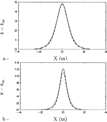
FIG. 5. Wave number modulations along the solitary wave 共X⫽0 at the solitary wave crest兲 predicted by WKBJ theory for the strong interaction of a 2 Hz shortwave共k⬁⫽16.09, h0⫽0.3 m兲 and a solitary wave of amplitude

A/h0⫽0.2025 共a兲 and A/h0⫽0.4129 共b兲 given by Byatt-Smith’s numerical

locity that this simple formula accurately reproduce the heu-ristic approach for solitary waves up to A/h0⫽0.4 and with less than 10% error up to A/h0⫽0.7.

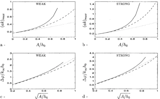
Finally, we have to compare the amplitude and wave number modulation obtained using each analytical approxi-mation of the solitary wave and the numerical solution. Wave number modulations共Fig. 5兲 associated with KdV show bet-ter agreement than Rayleigh with the modulations obtained using Byatt-Smith’s numerical solution. In all cases, the highest maximum wave number modulations are given using Byatt-Smith, with Rayleigh giving the lowest. The deviation between Rayleigh and Byatt-Smith at the maximum of wave number modulations reaches 40% for A/h0⫽0.5 in strong interaction. With respect to amplitude modulations 共Fig. 6兲, the deviation between Byatt-Smith and Rayleigh ranges from the double to four times the deviation between Byatt-Smith and KdV when solitary wave amplitude increases. Yet, Byatt-Smith predicts amplitude modulation at the solitary wave peak that are less than 6% greater than KdV 共for A/h0⫽0.5 in strong interaction兲. As a consequence of both wave number and amplitude modulations, when comparing steepness maxima at the crest of the solitary wave关Figs. 7共a兲 and 7共b兲兴, KdV and Byatt-Smith give close results up to A/h0⫽0.3. For A/h0⭓0.3, predicted steepness maxima are smaller for KdV than for Byatt-Smith. In all cases, using Rayleigh’s solution, predicted steepness maxima are smaller. Yet, the phase shifts deduced from wave number modula-tions given by Rayleigh are in better agreement with Byatt-Smith than KdV, as shown in Figs. 7共c兲 and 7共d兲. This is in line with our conclusion on particles displacements at the free surface. We suggest this is due to the better description of both the outskirts decay coefficient and the phase speed in Rayleigh solution 关see Figs. 3共a兲 and 3共b兲兴.

As a conclusion, granted that Byatt-Smith’s numerical solution is the exact solitary wave solution required in the theory, Rayleigh’s approximation appears to be better than KdV’s to test the short wave phase shift in the interaction with a solitary wave. But regarding Doppler effects and par-ticularly steepness prediction at the solitary wave crest, KdV would give a better approximation than Rayleigh.

III. EXPERIMENTAL PROCEDURE

The experiments are conducted in a 36 m long, 0.55 m wide, and 1.2 m high flume as sketched out on Fig. 8. It is equipped with two wave makers.

At one end of the flume a piston wave paddle can be displaced horizontally. The piston is linked to a hydraulic jack capable of a 600 mm stroke. The control system is monitored by a computer. Different motions of the paddle can be prescribed by the computer, enabling the generation of either solitary waves or sinusoidal waves. This ability was used for strong interactions when solitary waves and short waves need to be generated at the same end of the flume. Nevertheless the piston type wave maker, although not per-fect, is more appropriate for long wave generation rather than for short wave generation since it displaces the whole water column uniformly. Ideally, the piston would need to flex in such a manner as to reproduce the solitary wave vertical distribution of the velocity. This is not possible with our wave maker. However, we need to prescribe an appropriate law of motion for the paddle in order to produce solitary waves that are as pure as possible. Clamond and Germain10 used a law deduced from the first-order shallow water theory. All solitary waves generated with this motion exhibit a main pulse followed by a dispersive tail with no more than 10% of the amplitude of the leading pulse. In order to decrease the amplitude of the dispersive tail, different laws of motion for the piston wave maker were tested. It appears that solitary waves generated using a paddle motion law conforming to

共25兲 are purer 共smaller dispersive tail than with the original

law兲 and more rapidly established. Moreover, by reproducing different experiments concerning solitary wave generation with any generation law, we assess that it is highly reproduc-ible. So that for a given paddle law, we could know the solitary wave amplitude at any location in the flume given the probe accuracy. The law deduced from the Rayleigh so-lution implies larger paddle displacement than other laws. With regard to the finite stroke of the jack, this latter law lead to smaller solitary wave amplitudes. For a water depth of h0⫽0.3 m the upper bound of the solitary wave dimension-less amplitude is 0.35 while the first-order shallow water law allows a dimensionless amplitude up to 0.5.

For weak interactions, a plunging wedge wave maker was used to generate high-frequency monochromatic sinu-soidal waves. It is driven through a scotch-yoke共Welt28兲 by an electric motor rotating at constant speed. The frequency of the wedge motion ranges from 1 to 10 Hz. The amplitude of the motion is adjusted by prescribing a fixed eccentricity. This wave maker can be located at will anywhere along the flume. For the set of weak interactions, it was located at 28 m from the piston wave maker.

The depth at rest was fixed throughout the experiments at h0⫽0.3 m. It is a compromise between the capabilities of the solitary wave wave maker and the high frequency wedge wave maker. In addition for this depth the short wave has a dimensionless wave number k_⬁h0ranging from 2.73 to 7.54

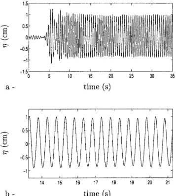
for frequencies varying from 1.5 to 2.5 Hz. It indicates that experiments were performed for intermediate to deep water depths conditions. The short wave is in fact a wave group as shown on Fig. 9共a兲. The front part is highly unstable. Enve-lope solitons can be generated in this front part and at least strong modulations of the amplitude are systematically ob-served. The central part of the record 关Fig. 9共b兲兴 shows a slight modulation in amplitude along with an asymmetry be-tween crests and troughs due to second-order nonlinearities. Harmonic analysis of this central zone shows that the first harmonic component is a very small fraction of the funda-mental component. Thus it is considered to be a nearly pure monochromatic wave. Care is taken so that the measurement of the interaction is made in the central part. Over 2.5 Hz the wave is severely damped and propagates no further than 3 m away from the plunging wave maker. It was noticed during

the experiments that damping was less pronounced after the tank had just been refilled, in other words when the free surface was clean. We thus attributed this damping to the free surface contamination, as Van Dorn29 already suggested. Thus, as it is not possible, given the size of the tank, to maintain the free surface clean enough, we did not proceed over 2.5 Hz.

Surface displacements during the experiments on the in-teraction between short surface waves and surface solitary waves are measured in fixed locations by resistive probes. Probe precision was estimated at 0.5 mm for free surface elevations lower than 5 cm and at 1 mm beyond this limit. This is due to probe calibration. These probes are combined in arrays and the distance between probes is fixed. The array can be moved along the flume, between 11 and 22 m from the piston wave maker depending on the experimental con-ditions. An extra probe can be dedicated to the measurement of the solitary wave before it has interacted. All experimental recordings of interactions are measurements of free surface displacement against time共between 15 and 25 seconds dura-tion兲. The probes are located along the center line of the

FIG. 7. 共a兲 and 共b兲 Steepness maxima at the crest of the solitary wave and 共c兲 and 共d兲 phase shifts deduced from wave number modulations predicted by WKBJ theory for weak and strong interaction of a 2 Hz short wave共k_⬁⫽16.09, h0⫽0.3 m兲 of amplitude 1 cm and a solitary wave given by Byatt-Smith’s

numerical solution共—兲, KdV 共- -兲, and Rayleigh 共¯兲.

FIG. 8. Sketch and dimensions of the experimental equipment.

flume to avoid lateral perturbations. We generate a solitary wave of amplitude A, a short wave of frequency f 共wave number k_⬁兲, and of amplitude a_⬁. A typical example of an interaction is presented on Fig. 10, on which four zones can be differentiated. Zone A is the recording of the short wave before interaction, zone B is the recording of the interaction between the solitary wave and the short wave when the soli-tary wave contribution is predominant, and zone C is the recording of the short wave after it has interacted. The slight modulation is due to the dispersive tail trailing the soliton. Zone D is a useless part of the recording. Indeed the reflected solitary wave interacts with the dispersive tail and the short wave.

From the theoretical point of view, we know that the short wave undergoes wave number modulations during the interaction. The modulations are difficult to obtain directly from the measurements. However, phase shift of the wave train A with respect to the wave train B is a consequence of

wave number modulations. The data processing to obtain this phase shift is based on a harmonic analysis technique de-tailed in Clamond and Barthe´lemy.11 This was found to be the most precise method. The methodology was tested on pure synthetic sinusoidal signals with no other contribution. In this case the phase shift between two arbitrary zones with such signals is 0 since no other wave is present. This method applied to such signals yields a phase shift as low as the machine roundoff error in double precision, namely 10⫺16rad. Concerning our experiments, we also tested the error induced by the dispersive tail that follows the solitary wave main pulse in zone C. To this end, two tests have been considered. First, we apply harmonic analysis to the super-imposition of a pure synthetic sinusoidal signal and a mea-sured free surface elevation for a single solitary wave. We considered solitary waves generated by the different paddle motion laws we tested. But in the whole range of solitary wave amplitude, the improvements in reducing the disper-sive tail did not show a significant reduction in phase shift error due to inaccuracy in the method because of the disper-sive tail. This error is at most 0.1 rad. Second, all interaction experiments were repeated with solitary waves generated ei-ther with Rayleigh or KdV paddle motion law. Phase shifts obtained from one or the other experiment series do not separate more than the error than can be estimated for a single experiment. Indeed a large contribution to the error comes from irregularities in the measured short wave signals. This was assessed by the following test. A record of a freely propagating short wave is split in two. Phase shift between both parts is computed. This was repeatedly done and it was found that phase shifts could reach 1.5 rad without any ap-parent disturbances. This error in phase computation is mainly attributed to uncertainties in the frequency determi-nation of short signals共records less than 10 s兲. The reliability of the frequency of the wave maker was checked. It was felt that the best way to estimate and reduce errors in phase shift determination was to repeat the measurements. All the phase shifts presented in this section are, therefore, an average on 5 or 6 values obtained at locations spanning 2 m共probe array兲. All the values presented fulfilled the criteria of an error lower than 1 rad, estimated from two times the standard deviation of the 5 or 6 values. Experiments for which this criteria was not fulfilled have been excluded. More details regarding ex-perimental errors can be found in Guizien.30 As mentioned above, given a short wave frequency and a solitary wave

FIG. 9. Recording of a high-frequency wave group at 10 m from the wedge wave maker; f⫽2 Hz, h0⫽0.3 m. 共b兲 is a close-up of the recording plotted

in共a兲 showing evidence of second-order contribution.

FIG. 10. Free surface elevation against time at 19.423 m from the piston wave maker; for the solitary wave A/h0⫽0.3 and the frequency of the short wave is f

⫽2.5 Hz 共k⬁⫽25.15兲 for an amplitude of a⬁ ⫽5.7 mm (h0⫽0.3 m).

amplitude, we carried out experiments for the different soli-tary wave laws of generation, considered as repetition of the same experiments. Besides, the short wave amplitude was also allowed to vary, from 4 to 12 mm, as long as the short wave out of the interaction was stable.

IV. RESULTS AND DISCUSSION

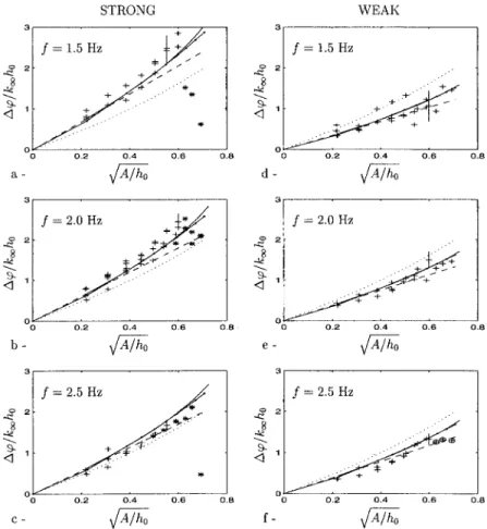
The interaction between a surface solitary wave and a short wave can be analyzed using very simple arguments, as recalled in the introduction. The short wave phase shift is then given by formula共31兲. We emphasize that this formula is obtained by considering only displacement due to solitary waves, linearly and instantaneously. As a consequence, the short wave direction of propagation is not taken into account. It should be noted that共31兲 is independent of the short wave amplitude a_⬁. Figure 11 shows the experimental results of nondimensional phase shifts ⌬␸/(k_⬁h0) against

冑

strong and weak interactions and various short wave frequen-cies. We do not identify on the plots of Fig. 11 the short wave amplitude. Indeed, it was not possible to show experi-mentally any dependency of the short wave phase shift on the short wave amplitude.

Heuristic phase shift⌬␸Hgiven by formula共31兲 is plot-ted as a dotplot-ted curve. In this representation, it is the same curve in all cases. Experimentally, weak interactions give smaller phase shifts than⌬␸Hwhile strong interactions give larger ones. Moreover it appears that for strong interactions the higher the frequency of the short wave, the closer the nondimensional experimental phase shifts are to

⌬␸H/(k⬁h0). This is not surprising since formula共31兲

as-sumes that the short wave does not propagate during the interaction. Indeed, this assumption is met with decreasing error as the frequency increases since then the short wave phase velocity also decreases. For weak interactions, since the induced phase shifts are smaller, it remains difficult to observe this effect as clearly. In order to clearly show this argument, we plot on Fig. 12 the relative deviation between phase shifts given by formula 共31兲 and experimental values or formula共9兲 for a Rayleigh solitary wave as the short wave wave number increases. In fact, this graph shows that the relative error one would do when using formula 共31兲 to es-timate the short wave phase shift, decreases when the short wave frequency increases. This error is less than 10% when

FIG. 11. 共⫹兲 Experimental phase shifts versus the square root of solitary wave dimensionless amplitudes; 共¯兲: ⌬␸H;共—兲: ⌬␸R;共- -兲: ⌬␸KdV;共—兲: ⌬␸BS;共*兲:

short wave was observed breaking; 共䊊兲: short wave suspected to be breaking from pictures;共a兲 strong and 共d兲 weak: f ⫽1.5 Hz; 共b兲 strong and 共e兲 weak: f ⫽2.0 Hz; 共c兲 strong and 共f兲 weak: f ⫽2.5 Hz with h0

⫽0.3 m.

FIG. 12. Relative deviation between phase shifts given by formula共31兲 and experimental values for共䊊兲: strong interaction; 共⫹兲: weak interaction and given by formulas共31兲 and 共9兲 for a Rayleigh solitary wave for 共—兲: strong interaction;共––兲: weak interaction.

k_⬁h0⭓30. However, the departure of ⌬␸_H from the dimen-sional phase shift increases when the short wave frequency increases as shown by Clamond and Germain.10This is be-cause the wave number increases more rapidly than the phase velocity decreases with increasing frequency.

On Fig. 11 we also plot the phase shifts⌬␸KdVgiven by formula 共21兲, ⌬␸R given by formula 共9兲 for a Rayleigh 共R兲 solitary wave and ⌬␸BS given by formula 共9兲 for a Byatt-Smith共BS兲 solitary wave. Up to A/h0⫽0.15, formulas 共21兲 and 共9兲 give very close results, which is in agreement with the KdV theory limit. Indeed, we already showed in Sec. II A how共9兲 reduces to 共21兲 under the small amplitude assump-tion. Formula 共9兲 for a Rayleigh or a Byatt-Smith soliton allows to predict phase shifts for a wider range of solitary waves, theoretically up to the limiting dimensionless ampli-tude of 0.8332共Longuet-Higgins25兲. In our experiments, we were limited to A/h0⭐0.5. In weak interactions, taking into account the experimental error共represented by the error bars on Fig. 11兲, it is not possible to conclude on a better agree-ment with one or the other formula. However, the advantages of this formulas appear for strong interactions when phase shifts are the largest. Indeed, the experimental results for large solitary waves in strong interaction are closer to pre-dictions of formulas 共9兲 共either based on the Rayleigh soli-tary wave approximation or Byatt-Smith numerical solution兲 for frequencies of 2 and 1.5 Hz. Repeated experiments 共es-pecially at 2 Hz兲 confirm this trend. For 2.5 Hz, this ten-dency is not as clear, partly due to the early breaking ob-served.

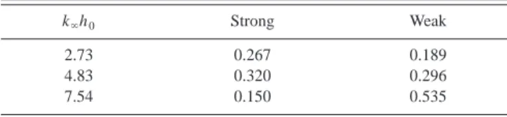
As a matter of fact, a 2.5 Hz short wave was observed ‘‘breaking’’ for a solitary wave of dimensionless amplitude A/h0⫽0.25 whereas for 2 and 1.5 Hz frequencies, breaking only occurred for the largest solitary waves, respectively, for A/h0⫽0.4 and A/h0⫽0.45. We use here the term breaking to refer to foam patches that one can see on the free surface. This breaking is due to the steepening of the short wave when both amplitude and wave number increase. Thus, short waves of different amplitudes but with the same frequency and interacting with the same solitary wave may be differen-tiated by breaking, whereas if only the phase shift is consid-ered they cannot. The maximum short wave steepness at the crest of the solitary wave when the short wave was observed breaking is computed from 共9兲 and 共10兲 using Byatt-Smith numerical solitary wave solution. These values bound to ex-perimentally observed breaking are given in Table II. We also report in Table II the maximum steepness values pre-dicted for the weak interaction with the largest solitary wave experimented (A/h0⫽0.5). Breaking was never clearly ob-served in our weak interactions 共no foam patches兲. Because of the uncertainty concerning the breaking limit, we may just stress that for the same predicted steepness for f⫽2.5 Hz (k_⬁h0⫽7.54), short waves are observed breaking in the strong interaction but not in the weak interaction case. More-over, the predicted steepness when breaking is observed is always smaller than the Stokes limit of 0.4461 for waves propagating at rest. This all suggests that breaking is not determined only by the steepness but also by the underlying velocities.

V. CONCLUSION

Theoretically we found a dispersion relation 共9兲 to de-scribe the wave number modulations of a short wave riding on a solitary wave that is similar to the one obtained for the refraction of waves in slowly varying media, except that it includes free surface elevation. Wave action conservation

共10兲 is also obtained. Any solitary wave solution may be

used and, if assuming a small amplitude one, Clamond and Germain’s10 analytical expression for the phase shift under-gone by the short wave is confirmed.

We compare short wave wave number and amplitude modulations obtained from 共9兲 and 共10兲 when using Byatt-Smith’s numerical solution and KdV or Rayleigh’s analytical solutions. The shape of the wave number modulation curve associated with KdV appears to be closer than Rayleigh to the one obtained with Byatt-Smith, but it misses the maxi-mum that occurs at the crest of the solitary wave for large solitary waves. Besides, phase shifts deduced from integra-tion under the curve for Rayleigh’s solitary waves are in better agreement with Byatt-Smith’s predictions than for KdV’s solitary waves. We suggest this is due to the better description in Rayleigh’s solution of the phase speed and outskirts decay coefficient. Another feature is that particles displacements at the free surface deduced from Rayleigh so-lution are very accurate. We thus derived a new analytical formula 共31兲 for the limiting case of high-frequency short waves riding on large amplitude solitary waves. Experimen-tally, strong interactions have been carried out for the first time. They clearly show the influence on the phase shift de-termination of the direction of propagation of the waves in-teracting as far as small wave number are concerned. Be-sides, the only case, when taking into account experimental error, measurements enable to show a better agreement with one of the theoretical formulas, occurs in strong interaction. Thus, we show in that case that ⌬␸R and ⌬␸BS were in better agreement than ⌬␸KdV with measurements. In addi-tion, we show that when the short wave wave number in-creases, phase shifts tends to the heuristic formula ⌬␸H. Indeed, in our experimental set, we covered a broader range of short wave wave number then Clamond and Barthe´lemy.11 During the experiments, some cases of breaking were observed that may be attributed to significant steepening of the short wave induced by both wave number and amplitude modulations. Indeed, breaking enables a difference to be made between two short wave trains with the same fre-quency but different amplitudes, whereas phase shift depends only on the frequency of the short wave. This latter appears

TABLE II. Maximum short-wave steepness at the crest of the solitary wave computed from共9兲 and 共10兲 when the short wave was observed breaking in strong interaction and for the largest solitary waves experimented (A/h0

⫽0.5) in weak interaction 共the short wave was NOT observed breaking in

these latter cases兲.

k_⬁h0 Strong Weak

2.73 0.267 0.189 4.83 0.320 0.296 7.54 0.150 0.535

in the theory and is confirmed by the experiments. Relying on theoretical predictions, the maximum steepness reached at the crest of the solitary wave can be estimated using Byatt-Smith’s numerical solution. It then appears that for similar maximum steepness predictions, short waves might be breaking in the strong interaction case whereas they do not in the weak interaction case, showing the influence of the un-derlying velocity.

ACKNOWLEDGMENTS

The authors would like to thank Jean-Marc Barnoud for technical support and assistance when performing the experi-ments. This work has been financially supported by the

MAST-III ECProgram, under Contract No. MAS3-CT95-0027.

1_{M. S. Longuet-Higgins and R. W. Stewart, ‘‘Changes in form of short}

gravity waves on long waves and tidal currents,’’ J. Fluid Mech. 8, 565

共1960兲.

2_{M. S. Longuet-Higgins and R. W. Stewart, ‘‘The changes in amplitude of}

short gravity waves on steady non-uniform currents,’’ J. Fluid Mech. 10, 526共1961兲.

3

C. J. R. Garrett, ‘‘Discussion: the adiabatic invariant for wave propagation in a non-uniform moving medium,’’ Proc. R. Soc. London, Ser. A 299, 26

共1967兲.

4_{F. P. Bretherton and C. J. R. Garrett, ‘‘Wave trains in inhomogeneous}

moving media,’’ Proc. R. Soc. London, Ser. A 302, 529共1969兲.

5

M. S. Longuet-Higgins, ‘‘The propagation of short-surface waves on longer gravity waves,’’ J. Fluid Mech. 177, 293共1987兲.

6_{M. Naciri and C. C. Mei, ‘‘Evolution of a short surface wave on a very}

long surface wave of finite amplitude,’’ J. Fluid Mech. 235, 415共1992兲.

7

J. Zhang and W. K. Melville, ‘‘Evolution of weakly non-linear short waves riding on long gravity waves,’’ J. Fluid Mech. 214, 321共1990兲.

8_{I.-F. Shen, W. J. Easson, C. A. Greated, and W. A. B. Evans, ‘‘The}

modu-lation of short waves riding on solitary waves,’’ Phys. Fluids 6, 3317

共1994兲.

9

W. A. B. Evans and M. J. Ford, ‘‘An exact integral equation for solitary waves共with new numerical results for some ‘internal’ properties兲,’’ Proc. R. Soc. London, Ser. A 452, 373共1996兲.

10_{D. Clamond and J.-P. Germain, ‘‘Interaction between a Stokes wave}

packet and a solitary wave,’’ Eur. J. Mech. B/Fluids 18, 67共1999兲.

11

D. Clamond and E. Barthe´lemy, ‘‘Etude expe´rimentale du de´phasage dans

l’interaction houle-onde solitaire,’’ C. R. Acad. Sci. Paris.共IIb兲 320, 277

共1995兲.

12_{J. W. Miles, ‘‘Obliquely interacting solitary waves,’’ J. Fluid Mech. 79,}

157共1977兲.

13

M. S. Longuet-Higgins and O. M. Phillips, ‘‘Phase velocity effects in tertiary wave interactions,’’ J. Fluid Mech. 12, 333共1962兲.

14_{Lord Rayleigh, ‘‘On waves,’’ Philos. Mag. 1, 257共1876兲.}

15_{D. J. Korteweg and G. De Vries, ‘‘On the change of form of long waves}

advancing in a rectangular canal, and on a new type of stationary waves,’’ Philos. Mag. 39, 422共1895兲.

16

J. G. B. Byatt-Smith, ‘‘An exact integral equation for steady surface waves,’’ Proc. R. Soc. London, Ser. A 315, 405共1970兲.

17_{M. A. Lavrentiev, ‘‘On the theory of long waves,’’ Translation A.M.S. 11,}

273共1962兲.

18_{J. H. Shyu and O. M. Phillips, ‘‘The blockage of gravity and capillary}

waves by long waves and currents,’’ J. Fluid Mech. 217, 115共1990兲.

19

M. W. Dingemans, ‘‘Water waves propagation over uneven bottom, Part 1-Linear wave propagation,’’ Advanced Series on Ocean Engineering

共World Scientific, Singapore, 1997兲, Vol. 13.

20

C. C. Mei, ‘‘The applied dynamics of ocean surface waves,’’ Advanced

Series on Ocean Engineering共World Scientific, Singapore, 1992兲.

21_{J. G. B. Byatt-Smith and M. S. Longuet-Higgins, ‘‘On the speed and}

profile of steep solitary waves,’’ Proc. R. Soc. London, Ser. A 350, 175

共1976兲.

22_{H. Lamb, Hydrodynamics, 6th ed. 共Cambridge University Press,}

Cam-bridge, 1932兲, p. 738.

23_{F. Serre, ‘‘Contribution a` l’e´tude des e´coulements permanents et variables}

dans les canaux,’’ La Houille Blanche 8, 374共1953兲.

24

C. H. Su and C. S. Gardner, ‘‘KdV equation and generalizations. Part III. Derivation of Korteweg–de Vries equation and Burgers equation,’’ J. Math. Phys. 10, 536共1969兲.

25

M. S. Longuet-Higgins, ‘‘Trajectories of particles at the surface of steep solitary waves,’’ J. Fluid Mech. 110, 239共1981兲.

26_{J. D. Fenton, ‘‘A ninth order solution for the solitary wave,’’ J. Fluid}

Mech. 53, 257共1972兲.

27_{M. S. Longuet-Higgins, ‘‘The trajectories of particles in steep,}

symmetri-cal gravity waves,’’ J. Fluid Mech. 94, 497共1979兲.

28

F. Welt, ‘‘Plunger-type wave makers for high frequency waves,’’ in

Roz-prawy Hydrotechniczne 共Polska Akademia Nauk-Instytut Budownictwa

Wodnego, 1990兲, pp. 139–146.

29

W. G. Van Dorn, ‘‘Boundary dissipation of oscillatory waves,’’ J. Fluid Mech. 24, 769共1966兲.

30_{K. Guizien, ‘‘Les ondes longues internes: ge´ne´ration et interaction avec la}