HAL Id: hal-00296987
https://hal.archives-ouvertes.fr/hal-00296987
Submitted on 26 Apr 2007
HAL is a multi-disciplinary open access
archive for the deposit and dissemination of
sci-entific research documents, whether they are
pub-lished or not. The documents may come from
teaching and research institutions in France or
abroad, or from public or private research centers.
L’archive ouverte pluridisciplinaire HAL, est
destinée au dépôt et à la diffusion de documents
scientifiques de niveau recherche, publiés ou non,
émanant des établissements d’enseignement et de
recherche français ou étrangers, des laboratoires
publics ou privés.
The combined use of weather radar and geographic
information system techniques for flood forecasting
E. Baltas
To cite this version:
E. Baltas. The combined use of weather radar and geographic information system techniques for
flood forecasting. Advances in Geosciences, European Geosciences Union, 2007, 10, pp.117-123.
�hal-00296987�
www.adv-geosci.net/10/117/2007/ © Author(s) 2007. This work is licensed under a Creative Commons License.
Geosciences
The combined use of weather radar and geographic information
system techniques for flood forecasting
E. Baltas
AUTH, Agricultural School, Department of Hydraulics, Soil Science and Agricultural Engineering, 540 06 Thessaloniki, Greece
Received: 10 September 2006 – Revised: 20 November 2006 – Accepted: 27 January 2007 – Published: 26 April 2007
Abstract. A distributed rainfall-runoff model capable for
real time flood forecasting utilizing highly spatial and time resolution data was developed. The study region is located under the WSR-74 S-band 100 km radar umbrella and is equipped with a number of rain gauge recording stations, a permanent installation for flow measurement and a stage recorder. The entire basin was digitized to 2×2 km2 grid squares by implying GIS techniques. A series of rainfall events recorded producing floods were analyzed and pro-cessed. The linear channel parameter assigned to each grid-square is based on its location measured by the centroid of the grid square along the channel network. The estimation of the hill-slope and the stream velocity are calculated based on the Geographic Information System (GIS) procedures.
1 Introduction
Flood flow forecasting for a catchment due to rainfall re-quires a quantitative estimate of precipitation. This can be accomplished using several methods including rain gauges, weather radar or a combination of rain gauges and weather radar. The traditional approach to flood forecasting is to use rainfall input estimated from a number of rain gauges driving a lumped parameter hydrological model. In rainfall-runoff transformation, lumped linear system models have been found to work, as well as, more physically based mod-els (Plate et al., 1988). O’Connell et al. (1986) have shown the utility of the semi-distributed models for on-line fore-casting of high resolution radar measurements. A number of mathematical models have been proposed by different au-thors to face the problem of flood forecasting (Baltas, 1998). In most of these models, combinations of linear conceptual elements are used to simplify the representation of
hydro-Correspondence to: E. Baltas
(baltas@agro.auth.gr)
logical processes. Hydrologists have always been interested in the effects of rainfall uncertainties on the accuracy and reliability of the estimation of catchment-scale hydrological variables (runoff peak discharge, volume, etc.). The recent advent of new technologies such as weather radar, satellites, Geographic Information Systems and high-speed computer workstations, provides new opportunities for improved hy-drological forecasting. This led to the development of dis-tributed models for flood forecasting (Baltas and Mimikou, 1999). In more complex approaches, models for rainfall pre-diction were also applied. Together with the development of more feasible strategies, they can assist the operation of human-made structures and flood warning systems. This new technology led to the development of models for flood forecasting and of more complex models incorporating cloud physics linked to mesoscale dynamical models to provide rainfall forecasts for many hours ahead (Baltas, 1998). Fur-thermore, the lumped nature of the model, gives an intrinsic weakness to the model to represent extremely uneven spatial rainfall distributions, making it necessary to work in smaller sub-basins in such cases (Yang et al., 2000). Measurement accuracy continues to be a problem, but have not prevented self-correcting hydrological models from being developed for operational use.
In this paper, a procedure is suggested for the real-time quantitative radar rainfall measurements used for flood sim-ulation and real-time flood forecasting. The model repre-sents the basin by grid squares of 2×2 km2 in area. Rain excess in each grid square is shifted linearly at the outlet of the basin. This model is an extension of the most common approach that is the division of a basin into sub-basins and channel segments and then the use of lumped rainfall-runoff models for the sub-basins and the combination of their re-sponses after routing through the appropriate channel seg-ments. Flood-flow forecasting in this area is very impor-tant because the region suffers from frequent and hazardous flash floods, causing damage and operational problems to
118 E. Baltas: Weather radar and geographic information system techniques for flood forecasting
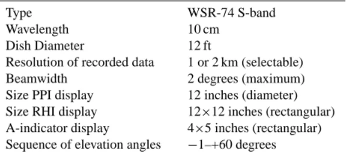
Table 1. The radar technical characteristics.
Type Wavelength Dish Diameter
Resolution of recorded data Beamwidth
Size PPI display Size RHI display A-indicator display
Sequence of elevation angles
WSR-74 S-band 10 cm 12 ft 1 or 2 km (selectable) 2 degrees (maximum) 12 inches (diameter) 12×12 inches (rectangular) 4×5 inches (rectangular) −1–+60 degrees
the downstream multipurpose reservoirs and agricultural and residential areas.
2 Study area and data processing
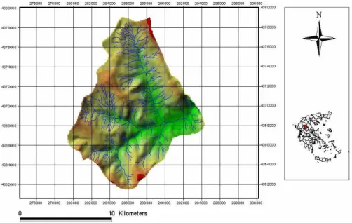
Flood phenomena in Greece usually are caused by intense rainstorms, whereas snowmelt is not a dominant factor in flood genesis. Most intense rainstorms are produced by the passage of depressions possibly accompanied by cold fronts (and rarely by warm fronts) approaching from W, SW or NW (Baltas and Mimikou, 1999). A convectional weather type (characterized by a cold upper air mass that produces dynamic instability) (Baltas, 1998a) is also responsible for many intense storms, especially in the summer period. The basin used in this study is the Pyli basin, located in the Thessaly water district under the 100 km radar umbrella with drainage area 135 km2(Fig. 1). The plain is traversed by Pin-ios river whose total catchment area is 10 500 km2, while the agricultural area is about 4000 km2. The orography of Pin-dos mountain range plays an important role in rainfall and runoff regimes in Greece. Thus, the mean annual rainfall ex-ceeds 1800mm in the mountainous areas of western Greece whereas in eastern regions of the country may be as low as 300 mm (Baltas, 1998b). This does not mean that extreme floods are uncommon in the relatively dry eastern part of Greece. Deforestation and urbanisation play an important role to flood genesis. They are responsible for the increas-ing severity and destructive power of floods. Deforestation, also related to soil erosion, is a major problem in Greece. It is noted that the percentage of the areas covered by forest today is 18%, while at the beginning of the nineteenth cen-tury it was more than 40% (Baltas and Mimikou, 1999). De-forestation was caused mainly from human activities such as fires, illegal land reclamation, pasturing, etc. The topography varies from narrow gorges to wide flood plains. Its vegeta-tion varies from grasslands to dense forest, while the climate is temperate and humid with substantial seasonal variation in temperature. Frequent and rapid changes in weather are caused by frontal air mass activity, resulting in frequent flash floods. Regarding the ground truth monitoring, the basin is
equipped with a number of hydrometeorological recording stations, as well as, stage recording stations along with per-manent installations for flow measurement at selected loca-tions in the river reach. Historical storm and flood events have been recorded and archived by the Public Power Cor-poration (PPC), the Ministry of Agriculture and the Ministry of Environment, Physical Planning and Public Works. These consist of hourly precipitation data from rain gauges and the corresponding streamflow rates at the outlet of the basin. Streamflow is estimated by using the hourly water level read-ings and the appropriate water level-discharge rating curves calibrated at the site. The Thiessen polygon methodology was used in order to derive the meteorological mean values over the catchment.
The radar involved in the study is a WSR-74 S-band weather radar located in a military base in the town of Larissa in Central Greece. From this radar site, a significant part of central and northern Greece is covered including the Pyli basin. A number of storm events included the ones that cre-ated flash floods, recorded every ten to thirty minutes, were analyzed and processed. A variety of factors causing system-atic random and range dependent errors are encountered in these estimates. After the suppression of the ground clutter map, the subtraction of the errors due to anomalous prop-agation, beam refraction and losses, interference of signal from other rain targets was carried out for rainfall estimation (Krajewski, 1987). The Marshall-Palmer Z-R exponential relationship was applied for the conversion of the radar re-flectivity data to rainfall estimates, considering R as the rain-fall on the ground and Z reflectivity factor measured by the radar. In the field of radar-rain gauge adjustment the Brandes method was developed for the need to merge radar and rain gauge rainfall information and thus to improve radar rainfall estimates, trying to explain quantitatively any discrepancies between the rainfall amounts indicated by the two different measurement techniques (Brandes, 1974).
A number of storm events creating flash floods were an-alyzed and processed. All these events belong to the same type of precipitation considered as cyclonic with moderate intensity, long duration and widespread rainfall distribution. Three dimensional polar coordinate maps of equivalent re-flectivity factor Z in dBZ values are recorded every ten to thirty minutes by the WSR-74 S-band radar. The most im-portant radar technical characteristics are shown in Table 1.
3 Radar rainfall estimation
The power received by the radar antenna from a rainfall tar-get is integrated in time and space to eliminate the charac-teristic fluctuation of the radar signal. The average received power can be expressed as:
Pr =CKZ/r2 (1)
Fig. 1. The Pyli basin.
where C is a constant depending on the parameters of the radar system and K is the attenuation constant. To obtain rain rate R, the reflectivity factor Z is used in a Z-R relationship of the form:
R = aZb (2)
where a and b are two parameters. Both Z and R are func-tions of the raindrop size distribution:
Z = Z ∞ 0 N (D)D6dD (3) and R = π 6 Z ∞ 0 D3N (D)w(D)dD (4)
where D is drop diameter, N (D) is raindrop size distribution and w(D) is a function describing terminal velocity of rain-drops. It is obvious from the analysis of Eqs. (3) and (4) that even for the simple, two-parameter exponential distribution:
N (D) = Noexp(−3D) (5)
there is no unique relationship between Z and R, therefore, rainfall estimation based on (2) will lead to errors. However, there is a variety of factors that can cause systematic, random and range dependent errors. A short list of factors affecting the accuracy of rainfall derived from radar measurements is shown below (Zawadski, 1984):
1. High variability of raindrop size distribution which de-termines the Z-R relationship.
2. Changes in the vertical reflectivity profile.
3. Bright band effects caused by scattering of radar waves by ice particles present in the higher levels of some clouds.
4. False echo caused by anomalous propagation of radar waves.
5. Miscalibration of radar electronic instruments. 6. Erroneous measurements of the Pr.
7. Atmospheric processes between the level of the mea-surement cell and the ground.
4 Processing of the weather radar data
The raw radar data measured in polar co-ordinates in dBZ values are converted to Cartesian ones with grid dimensions 2×2 km2. A large area under the radar umbrella suffers from ground echoes which is a fact prohibiting radar utilization for such areas. Since the WSR-74 S-band radar system is not “dopplerized”, a ground clutter map measured during a cloudless sky in the optimum elevation, was utilized for the detection and suppression of the ground clutter from radar rainfall fields. After the averaging of radar reflectivity data in whole hours, the well known Marshall-Palmer Z-R ex-ponential relationship was applied for the conversion of the radar reflectivity data to rainfall estimates. The reason that the Marshall-Palmer relation was used is that all the events analyzed and processed are found after implying (off-line) least square methods to have a ranging from 170 to 215 and
b from 1.2 to 1.6 relatively close to the Marshall-Palmer
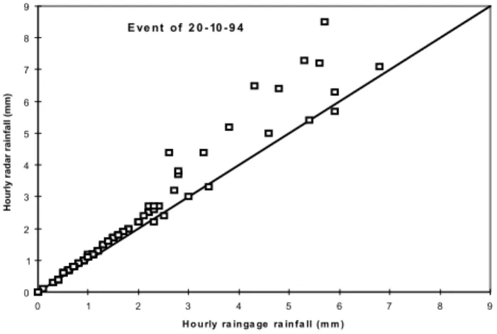
120 E. Baltas: Weather radar and geographic information system techniques for flood forecasting E ve n t o f 2 0 - 10 - 9 4 0 1 2 3 4 5 6 7 8 9 0 1 2 3 4 5 6 7 8 H o u rly ra in ga ge ra in fa ll (m m ) H o u rl y r a d a r ra in fa ll (m m ) 9
Fig. 2. One-to-one correspondence between the mean rain gauge
hourly and the mean radar hourly rainfall.
derived for the various locations of the rain gauge stations considering R as the rainfall on the ground and Z reflectivity factor measured by the radar.
The next step is the application of the influence function method (Krajewski, 1987). It is applied to solve the problem of outliers detection resulting from errors due to abnormal beam refraction and losses, some type of anomalous propa-gation and interference of signal from other than rain targets. The influence function method is based on analysis of spa-tial correlation in the field and applied to radar rainfall fields. The reason that this method was selected is that applied to the same type of precipitation considered as cyclonic, doesn’t re-quire any external information or calibration, as well as any knowledge of distribution of the data and can be fully auto-mated and used in an on line mode.
5 Radar rain gauge combination
In order to cope with biases in radar rainfall estimate the joint use of radar and rain gauge data has been recommended (Doviak and Zrnic, 1984). Joint use of radar and rain gauge data aims at the utilization of the high point accuracy of the latter and the wide area coverage of the former.
An approach based on the Brandes method was developed for the need to merge radar and rain gauge rainfall infor-mation and thus, to improve radar rainfall estimates, try-ing to explain quantitatively any discrepancies between the rainfall amounts indicated by the two different measurement techniques. The main characteristics of the Brandes method (Brandes, 1974), based on G/R ratio, is the comparison be-tween radar and rain gauge measurements in order to achieve adjustment factors which are used to force radar estimates to agree with rain gauge observed values. In this method an adjustment factor derived by using the rain gauges lo-cated in a selected range around that point is assigned to each
grid point. The adjustment factor F1at each grid point is a
weighted mean of the N rain gauge observations:
F1= N X i=1 WT iGi/ N X i=1 WT i ! (6)
where WT iis a weight function depending on the range from
the rain gauge to the grid point r given by:
WT i=exp(−r2/EP ) (7)
where EP is a filtering parameter considered constant. In all storm events after the processing of the radar data, the comparison of the hourly estimated radar rainfall to the hourly measured rain gauge rainfall are relatively close, as representatively shown in Fig. 2 for the event occurred on 20-10-94.
6 Form of the distributed grid model
The basin is divided into N grid squares. Each grid square is assumed to transform excess rain by a transfer function. The transfer function is defined by a series of combination of linear channels and a linear reservoir. The linear channel parameter is a function of the location of the grid square. The linear reservoir parameter is assumed to be the same for all grid squares. The time of first rise at the observed hydrograph decides the time of start of rainfall excess in each grid square. The contribution of a grid square at time t is given by the equation: Qt = i=t −(tC,g+λ) X j =tr−(tC,g+λ) Rj,gUi−j +1 (8)
Combining the contribution of all grid squares for which i>0 gives Qt = N X g=1 i=t −(tC,g+λ) X j =tr−(tC,g+λ) Rj,gUi−j +1 (9)
where N is the number of grid squares, Qt is the computed
discharge at time t and Ut are discrete values computed
as-suming the response function to be a linear reservoir. Rainfall excess is computed using two infiltration models. These models consider the rain prior to the time tr−(tc,g+λ)
as initial loss. In the first scheme, the abstraction rate is con-sidered constant. In the second scheme, the Philip’s equation is used to define the infiltration process and the parameters are assumed to be the same for each grid square.
The Philip’s equation is given by:
F = St0.5+At (10)
or
f = 1
2St
−0.5+A (11)
where S is called sorptivity, a function of initial and surface water contents of the soil and soil-water diffusivity, A is a parameter depending upon soil properties, F is the accumu-lated infiltered water as time t elapses and f is the infiltration rate.
The resulting equations incorporating the infiltration schemes are: Qt = N X g=1 i=t −(tC,g+λ) X j =tr−(tC,g+λ) (Pj,g−8)Ui−j +1 (12) and Qt = N X g=1 i=t −(tC,g+λ) X j =tr−(tC,g+λ) (Pj,g−S(t0.5−(t − 1)0.5) − A)Ui−j +1 (13) where Pj,g is the precipitation at time j on grid g, 8 is the
average abstraction rate, S is the sorptivity and A is a con-stant parameter for Philip’s method.
7 Estimation of the parameters
The parameters of the model represented by Eq. (12), are λ,
tc,g, K and F and those represented by Eq. (13), are λ, tc,g, K, S and A. The parameters which are determined off-line
are λ, tc,g and A. The parameter λ denotes the initial lag
and is a time delay parameter taken the same for all grids (Fattorelli and Scaletta, 1991). The parameter tc,g is a time
parameter assigned to each grid square on the basis of its lo-cation measured by the centroid of the grid square along the channel network. The tc,gvalues were derived based on
his-torical events through two different ways, first by using var-ious pairs of velocities off-channel and in channel network and secondly by implying the Nash hydrograph to the histor-ical events.
First, the linear channel parameter assigned to each grid square is based on its location measured by the centroid of the grid square along the channel network. The time to the outlet of the basin is given as follows:
t = Sh/Vh+Ss/Vs (14)
where Sh the distance from the center of the grid to the
stream, Ss the distance from the stream for each grid to the
exit of the basin, Vhthe hill slope velocity and Vsthe stream
velocity.
The estimation of the hill slope and the stream velocity are calculated based on GIS procedures. These values were calibrated based on the unit hydrograph which was derived based on historical events.
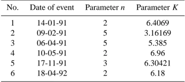
The later helped through the calculation of the first and second moment arms of the excess rainfall and direct runoff hydrograph to the estimation of the Nash parameters n and
K for each flood event. Table 2 shows the derived values of n
Table 2. The derived values of n and K for each flood event.
No. Date of event Parameter n Parameter K
1 14-01-91 2 6.4069 2 09-02-91 5 3.16169 3 06-04-91 5 5.385 4 10-05-91 2 6.96 5 17-11-91 3 6.30421 6 18-04-92 2 6.18
and K for each flood event. A mean value of both parameters was used for the construction of the response formation h(t) with time.
The third parameter estimated off-line, is the parameter of Philip’s infiltration scheme A, a function of the soil prop-erties and equals to the 2/3 of hydraulic conductivity term (Singh, 1992).
The parameters which are to be estimated on line have been identified as F and K in the first infiltration scheme and S and K in the second scheme. The on line estimation of the parameter is performed based on the minimization of an objective function. This objective function is the summation of the square differences between the observed and computed flows.
Each grid square operates as a linear reservoir model, a one parameter (K) model. The form of the instantaneous unit hydrograph of a linear reservoir is the following:
h(t ) = 1
Ke
−t /K (15)
Convoluting any input with the system response given in Eq. (15) and implying a conversion unit factor, will result in the corresponding discharge in m3/s. The response function will be hourly integrated for the estimation of the discrete values Ut.
The criteria that are used in order to optimize the initial values of the parameters concern the minimization of an ob-jective function, defined as the summation of the squares of differences between the observed and estimated discharge each time step. The objective function which is minimized during the optimization of the parameters is the following: Objective function = ((Qobj(i) − Qcomp(i))2W T (i))0.5/N0.5
(16) where Qobj(i) = the observed discharge in time i, Qcomp(i) = the computed discharge in time i, W T (i) = the weight co-efficient for ordinate i and N = the total number of ordinates. For the estimation of the discharge in each time step, the number of ordinates taken into account for the minimization of the objective function is limited and is given based on the weight coefficient defined by the following equation:
j2
122 E. Baltas: Weather radar and geographic information system techniques for flood forecasting 0 10 20 30 40 50 60 0 20 40 60 80 100 1 Time (hours) D is ch a rg e (m ^3 /s e c) 20 Observed
Compuyed by using the constant losses method Computed by using the Philip's method
vent 25-12-93
Fig. 3. The simulated hydrographs by using the constant losses and
the Philip’s method versus the observed.
Figure 4. The simulated hydrographs by using the constant losses and the Philip’s
0 10 20 30 40 50 60 70 80 90 0 10 20 30 40 50 60 70 80 90 100 Time (hours) D is ch a rg e (m ^3 /s ec ) Observed
Computed by using the constant losses method Computed by using the Philip's method
vent 20-10-94
Fig. 4. The simulated hydrographs by using the constant losses and
the Philip’s method versus the observed.
where j = the number of time steps 1T from the beginning of the period used for the calculation of the parameter.
8 Results
Model runs were performed in two phases. First in the sim-ulation phase and second in the forecasting phase. Equa-tions (12) and (13) were used to simulate the hydrographs. Representative results for the simulation phase using both the mean constant losses method and the Philip’s one, as well for the two of the events examined, are shown in Fig. 3 and 4. In these figures one can observe the relatively good agree-ment between the observed and computed hydrographs. The stochastic error component computing the time series of error between the observed and computed values from the time of first rise of the hydrograph until the time of forecast, was em-ployed. The time series were analyzed to obtain the correla-tion structure for fitting an autoregressive model. The AR(1)
0 10 20 30 40 50 60 70 80 90 0 5 10 15 20 25 30 Time (hours) D is ch a rg e (m ^3 /s ec ) Observed Computed
4-hour forecasted by using the constant losses method
vent 20-10-94
p
Fig. 5. Four-hour flood forecasting using the constant loss method.
0 10 20 30 40 50 60 70 80 90 0 5 10 15 20 25 30 Time (hours) D is ch a rg e ( m ^3 /s e c) Observed Computed
4-hour forecasted by using the Philip method
vent 20-10-94
Fig. 6. Four-hour flood forecasting using the Philip’s method.
and AR(2) models were selected. The parameters were deter-mined and checked for stationarity. If the parameters of the AR(2) model do not satisfy the stationarity condition, then the AR(1) model is used. The standard deviation of the resid-ual series is also computed for the evaluation of the AR(1) and AR(2) models and for the selection of one of these. The parameters of the autoregressive model are now used to com-pute the forecast errors beyond the time of forecast. These errors are added to the computed forecast discharges. Fore-casts were carried out by setting lead time equal to two and four-hour ahead, covering the rising limb until the peak had passed with results of acceptable accuracy. Representative results for the four-hour flood forecast using the mean con-stant losses and the Philip’s method are shown in Fig. 5 and 6 respectively.
9 Conclusions
The main conclusions derived from this research work are concentrated on the following:
1. A series of storm events creating flash floods were an-alyzed and processed. The entire basin was divided in grid squares of dimensions 2×2 km2. An adaptive grid-square-based flood-forecasting model capable of utilizing rainfall information on each grid square using weather radar, is proposed. Two different ways (one us-ing GIS methods and one by implyus-ing the Nash hydro-graph) were used to define the time delay of each grid square to the outlet of the basin. The model is able to formulate simulated hydrographs with relatively close agreement to the observed ones, as well as acceptable forecasts with a maximum lead time of 4 h. The 4 h time period is little less than the time delay between the occurrence of effective rainfall and the production of its main effects at the Pyli basin.
2. Two infiltration schemes have been used to compute the rainfall excess. It emerges from the study that the grid model using the average abstraction rate as the infiltra-tion model computes better forecasts for the majority of the flood events analyzed.
3. The updating of the parameters was performed in real time, every time step minimizing an objective function. This objective function is a summation of the square dif-ferences between the observed and computed discharge values. The autoregressive model was implied for the simulation of the error term.
Edited by: S. C. Michaelides and E. Amitai Reviewed by: anonymous referees
References
Baltas, E. and Mimikou, M.: A Grid-based rainfall-runoff model for flood forecasting, Proc. III International Symposium on Hydro-logical Applications of Weather Radars, Sao Paolo Brazil, Au-gust 1995.
Baltas, E.: Distributed modeling of river basin runoff in Greece, Radar Hydrology for Real Time Flood Forecasting, An Ad-vanced Study Cource, University of Bristol, UK, 24 June–3 July, 1998, 1998a.
Baltas, E.: Radar based for real-time flood forecasting in the Pin-ios river basin, in: International RIPARIUS Workshop on “Flood Risk Assessment, Communication, Present Practice and Future Needs”, Brussels, 27–28 October, 1998, pp. 99–111, 1998b. Baltas, E. and Mimikou, M.: Comparison of rainfall – runoff
mod-els based on spatial rainfall, Hydrotechnika, Hellenic Hydrotech-niki Union, 9, 27–40, 1999.
Brandes, E. A.: Optimising rainfall estimates with the aid of radar, J. Appl. Meteor., 14, 1339–1345, 1974.
Doviak, R. J. and Zrnic, D. S.: Doppler radar and weather observa-tions, Academic Press, Orlando, Florida, 1984.
Fattorelli, S. and Scaletta M.: Real-time flood forecasting mod-els intercomparison, Advances in Radar Hydrology, International Workshop, Lisbon, 11–13 November, 1991.
Krajewski, W. F.: Radar rainfall data quality control by the in-fluence function method, Water Resour. Res., 23(5), 837–844, 1987.
O’ Connell, P. E., Brunsdon, G. P., Reed, D. W., and Whitehead, P. G.: Case studies in real-time hydrological forecasting from the UK, in: River flow modelling and forecasting, edited by: Krai-jinhoff, D. A. and Moll, J. R., Reidel, Dordrecht, pp. 195–238, 1986.
Plate, E. J., Ihringer, J., and Lutz, W.: Operational models for flood calculation, J. Hydrol., 100, 489–506, 1989.
Singh, P. V.: Elementary Hydrology, Prentice Hall, Englewood Cliffs, N.S., 1992.
Zawadzki, I.: Factors affecting the precision of radar measurements of rain, Preprints of the 22nd Conference on Radar Meteorology, American Meteorological Society, Boston, Massachusetts, 1984. Yang, D., Herath, S., and Musiake K.: Comparison of different dis-tributed hydrological models for characterization of catchment spatial variability, Hydrol. Processes, 14, 403–416, 2000.