HAL Id: insu-01164979
https://hal-insu.archives-ouvertes.fr/insu-01164979
Submitted on 18 Jun 2015
HAL is a multi-disciplinary open access
archive for the deposit and dissemination of
sci-entific research documents, whether they are
pub-lished or not. The documents may come from
teaching and research institutions in France or
L’archive ouverte pluridisciplinaire HAL, est
destinée au dépôt et à la diffusion de documents
scientifiques de niveau recherche, publiés ou non,
émanant des établissements d’enseignement et de
recherche français ou étrangers, des laboratoires
Arrowsmith, Collin Bode, Christopher Crosby, Stephen Delong, Nancy Glenn,
Sara Kelly, et al.
To cite this version:
Paola Passalacqua, Patrick Belmont, Dennis Staley, Jeffrey Simley, J. Ramon Arrowsmith, et
al..
Analyzing high resolution topography for advancing the understanding of mass and energy
transfer through landscapes: A review. Earth-Science Reviews, Elsevier, 2015, 148, pp.174-193.
�10.1016/j.earscirev.2015.05.012�. �insu-01164979�
ACCEPTED MANUSCRIPT
Analyzing high resolution topography for advancing the
understanding of mass and energy transfer through
landscapes: A review
Paola Passalacquaa,∗, Patrick Belmontb, Dennis M. Staleyc, Jeffrey D. Simleyc,
J Ramon Arrowsmithd, Collin A. Bodee, Christopher Crosbyf, Stephen B.
DeLongg, Nancy F. Glenni, Sara A. Kellyb, Dimitri Laguej, Harish
Sangireddya, Keelin Schaffrathb, David G. Tarbotonk, Thad Wasklewiczl,
Joseph M. Wheatonb
aDepartment of Civil, Architectural, and Environmental Engineering and Center for
Research in Water Resources, The University of Texas at Austin, 301 E. Dean Keeton St. STOP C1700 Austin, TX 78712-2100, USA
bDepartment of Watershed Sciences, Utah State University, 5210 Old Main Hill, NR 350
Logan, UT 84322-5210, USA
cU.S. Geological Survey, Golden CO, USA
dSchool of Earth and Space Exploration, Arizona State University, 1151 S. Forest Ave.,
Tempe, AZ 85281 USA
eDepartment of Integrative Biology, University of California Berkeley, Valley Life Sciences
Bldg 3140, Berkeley CA 94720-3140 USA
fUNAVCO, 6350 Nautilus Drive, Boulder, CO 80301-5394 USA
gU.S. Geological Survey, 345 Middlefield Road, Menlo Park, CA 94025-3561 USA
hDepartment of Geosciences, Boise State University, 1910 University Drive Boise, ID
83725-1535 USA
iDepartment of Geosciences, Boise State University, 1910 University Drive Boise, ID
83725-1535 USA
jG´eosciences Rennes, Universit´e Rennes 1, UMR6118 CNRS, Campus de Beaulieu, 35042
Rennes Cedex, France
kDepartment of Civil and Environmental Engineering, Utah State University, 5210 Old
Main Hill, NR 350, Logan, UT 84322-5210, USA
lDepartment of Geography, A-204 Brewster Hall, East Carolina University, Greenville, NC
27858, USA
Abstract
The study of mass and energy transfer across landscapes has recently evolved to comprehensive considerations acknowledging the role of biota and humans as geomorphic agents, as well as the importance of small-scale landscape features. A contributing and supporting factor to this evolution is the emergence over the last two decades of technologies able to acquire High Resolution Topography
∗Corresponding author
ACCEPTED MANUSCRIPT
(HRT) (meter and sub-meter resolution) data. Landscape features can now be captured at an appropriately fine spatial resolution at which surface processes operate; this has revolutionized the way we study Earth-surface processes.
The wealth of information contained in HRT also presents considerable chal-lenges. For example, selection of the most appropriate type of HRT data for a given application is not trivial. No definitive approach exists for identifying and filtering erroneous or unwanted data, yet inappropriate filtering can create arti-facts or eliminate/distort critical features. Estimates of errors and uncertainty are often poorly defined and typically fail to represent the spatial heterogeneity of the dataset, which may introduce bias or error for many analyses. For ease of use, gridded products are typically preferred rather than the more information-rich point cloud representations. Thus many users take advantage of only a fraction of the available data, which has furthermore been subjected to a series of operations often not known or investigated by the user. Lastly, standard HRT analysis work-flows are yet to be established for many popular HRT operations, which has contributed to the limited use of point cloud data.
In this review, we identify key research questions relevant to the Earth-surface processes community within the theme of mass and energy transfer across landscapes and offer guidance on how to identify the most appropriate topographic data type for the analysis of interest. We describe the operations commonly performed from raw data to raster products and we identify key considerations and suggest appropriate work-flows for each, pointing to use-ful resources and available tools. Future research directions should stimulate further development of tools that take advantage of the wealth of information contained in HRT data and address present and upcoming research needs such as the ability to filter out unwanted data, compute spatially variable estimates of uncertainty and perform multi-scale analyses. While we focus primarily on HRT applications for mass and energy transfer, we envision this review to be rel-evant beyond the Earth-surface processes community for a much broader range of applications involving the analysis of HRT.
ACCEPTED MANUSCRIPT
Keywords: lidar, geomorphic features, change detection, point cloud, InSAR,
IfSAR, bathymetry, Structure from Motion, filtering
1. Introduction
One of the fundamental principles for understanding Earth-surface processes is conservation (Anderson and Anderson, 2010); the total rate of change of a quantity, such as mass or energy, within a control volume equals the rate of change of the quantity stored within the control volume plus the quantity net
5
outflow across the control surface. Rates of change depend on sources and sinks of the quantity of interest and on spatial gradients in transport rates. Many problems of interest to geomorphologists and hydrologists can be cast in these terms (Kirkby, 1971). Development of a sediment budget of a watershed, for example, requires the identification of sediment sources and sinks, and the
10
understanding of how sediment is transformed and transported from one point of the watershed to another.
The ability to predict water, sediment, and nutrient transfer, map natu-ral hazards, perform a radiation balance, and understand biophysical feedbacks that control landscape form and function is of great value to Earth-surface
15
scientists and natural resources managers. This ability relies on the under-standing of how mass and energy are transferred through watersheds and land-scapes. Contributions on this topic have populated the geomorphologic and hydrologic literature for over a century (Gilbert and Dutton, 1880; Davis, 1892; Gilbert, 1909; Gilbert and Murphy, 1914; Strahler, 1952; Culling, 1960; Kirkby,
20
1971; Smith and Bretherton, 1972; Willgoose et al., 1991a,b,c; Anderson, 1994; Howard, 1994; Tucker and Slingerland, 1994, 1997; Dietrich et al., 2003) which also account for the effect of biota and humans on landscapes. A large set of field observations and models, in fact, supports the knowledge that biological pro-ductivity affects directly and indirectly landscape evolution (e.g., Drever, 1994;
25
Butler, 1995; Gabet, 2000; Lucas, 2001; Sidle et al., 2001; Bond et al., 2002; Meysman et al., 2006; Yoo et al., 2005; Phillips, 2009; Foufoula-Georgiou et al.,
ACCEPTED MANUSCRIPT
2010). Humans, long recognized as geomorphic agents (Marsh, 1869, 1882), have now significantly impacted landscapes and their ecosystems (Hooke, 1994, 2000; Foley et al., 2005; Ellis et al., 2006; Montgomery, 2007; Syvitski and Saito, 2007;
30
Wilkinson and McElroy, 2007; Ellis, 2011; Sidle and Ziegler, 2012; Tarolli et al., 2014). Roads, for example, can play an important role in a watershed sediment budget as they constitute a significant source of sediment (Sidle and Ziegler, 2012) and disrupt ecosystem connectivity (Riitters and Wickham, 2003).
The evolution in mass and energy transfer studies is also reflected in
mathe-35
matical modeling approaches. From the employment of classic mass and energy conservation laws (Eagleson, 1986; Lane, 1998; Trimble, 1999; Dietrich et al., 2003), recent years have also seen the development of nonlocal constitutive laws expressing the material flux at a point (e.g., sediment flux) as a function of the conditions in some neighborhood around this point in space and/or in time
40
(e.g., Bradley et al., 2010; Foufoula-Georgiou et al., 2010; Ganti et al., 2010;
Tucker and Bradley, 2010; Foufoula-Georgiou and Passalacqua, 2013; Furbish and Roering, 2013). The nonlocal approach allows incorporating the heterogeneity and
com-plexity typical of geomorphic systems and the wide range of spatial and temporal scales that characterizes geomorphic processes.
45
Topographic gradients are a key factor in the transport of mass and energy. Whether computed at the location of interest or over a domain of influence as in nonlocal approaches, topographic attributes, such as slope, curvature, and roughness, play a fundamental role in the transport of mass and energy through landscapes. In the past, however, the representation of the Earth-surface was
50
possible only at coarse spatial resolutions (i.e., ≥ 10 m). Data collected dur-ing the Shuttle Radar Topography Mission (SRTM data), for example, were a major breakthrough in the early 2000s, but are quite coarse (30 m resolution) compared to today’s standards. SRTM data do not capture many of the small scale features and perturbations, both natural and anthropogenic, that combine
55
to exhibit significant control over mass and energy transfer. This applies also to the US Geological Survey’s National Elevation Dataset that has traditionally only been available at 10 m and 30 m resolutions.
ACCEPTED MANUSCRIPT
The explosion of availability of high resolution topography (HRT) over the last two decades is revolutionizing the way we study mass and energy transfer
60
through landscapes. We define HRT as any topographic dataset, which in its raw form consists of location (x,y) and elevation (z) measurements that collectively comprise a point cloud, and which have average spatial resolutions greater than or equal to one point per square meter (needed to achieve at least meter scale representation of the terrain). Thus, features in the landscape can be accurately
65
characterized and quantified at the fine spatial resolutions at which many hy-drologic, geomorphic, and ecologic processes occur. HRT data can be obtained remotely from various mobile platforms (e.g., planes, boats, vehicles) or static platforms (e.g., a tripod on the ground), using different techniques (e.g., Light Detection and Ranging (LIDAR), Synthetic Aperture Radar (SAR), Structure
70
from Motion (SfM), SOund Navigation And Ranging (SONAR)).
While remotely sensed HRT data are not a substitute for other forms of field observations (Roering et al., 2013), they do markedly enhance our ability to study Earth-surface processes quantitatively (Tarolli, 2014); an example is the emergence of characteristic scales of geomorphic processes (Perron et al.,
75
2009; Gangodagamage et al., 2011, 2014). In addition to the characterization of landscape structure through feature detection, identification, and extraction, HRT data allow capturing kinematic and dynamic changes of the Earth’s sur-face through differencing of data sets acquired at different times. An example is the ability to measure surface displacements and rotations due to earthquakes
80
(Nissen et al., 2012; Oskin et al., 2012; Glennie et al., 2014). The variability and complexity of landscapes, particularly at large scales (Rhoads, 2006) and over time can be fully embraced with HRT data. Preliminary mapping can be performed over vast areas from a personal computer and can be used to identify specific locations of interest to be subsequently field surveyed. The completeness
85
of HRT also offers the opportunity to advance process-understanding through change measurement (e.g., vegetation development, sedimentation, bank ero-sion) and heterogeneity characterization (e.g., vegetation, rockfall size distribu-tion).
ACCEPTED MANUSCRIPT
In addition to these substantial advantages, working with HRT data presents
90
significant challenges. Given that numerous combinations of platforms and tech-niques for HRT acquisition exist, users often have little basis for determining which platforms are best for their specific application (Bangen et al., 2014). For many applications (e.g., fluvial environments), no single HRT platform or technique paints a complete topographic picture and instead multiple techniques
95
are combined (Williams et al., 2014). Raw HRT data post processing techniques and related parameters are often not known to the earth scientist end-user and frequently not made available from the data provider. What operations are per-formed on raw data to create a usable point cloud? What further operations are needed to create a Digital Terrain Model (DTM)? Can geomorphic features be
100
extracted automatically and objectively? How does one quantify change over time from point cloud or rasterized data? Despite the rapidly growing avail-ability of HRT data, scientific discovery and applications of HRT data analyses to directly inform natural resource policy and management have been limited. Tools for extracting useful information from HRT data have been developed
105
and new ones are under development, but the Earth Sciences community lacks guiding principles and standard analysis work-flows as well as best practices for determining and reporting HRT data quality. These factors have resulted in a knowledge gap that separates HRT viewers and HRT analysts.
With this review, we wish to reduce this knowledge gap. In the material
110
that follows, we offer an overview of available data types and guidance on how to choose the most appropriate HRT data platform for the application at hand. We identify sources of error and work-flows to account for uncertainty. We discuss the operations that are commonly, or should be, performed in convert-ing raw data to point clouds to raster products and how the analysis of mass
115
and energy transfer through landscapes has changed with HRT data. It is not our goal to provide a comprehensive review of HRT acquisition and HRT-based research, which have been recently provided by Glennie et al. (2013b), Roering et al. (2013), and Tarolli (2014). We also narrow our focus to the anal-ysis of mass and energy transfer across landscapes, but many of the ideas and
ACCEPTED MANUSCRIPT
tools presented in this review will be relevant to other facets of the Earth-surface processes community and beyond.
The paper is organized in four main sections. The ‘Ask’ section (Section 2) covers HRT data sources, how to choose the most appropriate data type, critical questions to ask when acquiring a new HRT dataset or attempting to determine
125
the quality of an existing HRT dataset, and key considerations to account for uncertainty. The ‘Do’ section (Section 3) is focused on the operations performed from raw data to point clouds to raster products, work-flows for feature and change detection, and broad considerations on mass and energy transfer studies with HRT. The ‘Next’ section (Section 4) explores the next generation of HRT
130
data, opportunities for development of appropriate analysis tools, and needs to further our understanding of mass and energy transfer through landscapes. Finally, we offer guiding principles for HRT analysis in Section 5.
2. ASK: Considerations for planning HRT acquisition or working with previously collected HRT data
135
Use of HRT data poses challenges for the Earth science community; however, these can be mitigated with a fuller understanding of data characteristics, for-mats, provenance, and by identification of proper tools to measure data quality, manipulate and analyze data and address the scientific question of interest. In this section, we address important factors to consider when acquiring new
140
data, including what should be standard requirements for new data acquisition, whether you are acquiring the HRT data yourself or requesting from a com-mercial vendor, as well as what information is needed to assess the quality of data previously collected by someone else. We offer an overview of the types of available HRT, their characteristics, and guidance on how to choose the most
145
appropriate HRT for the application at hand. We then discuss sources of un-certainty and present strategies for unun-certainty assessment of data and data processing. The main steps to obtain derived products (workable point clouds and rasters) from raw data will be presented in Section 3.
ACCEPTED MANUSCRIPT
2.1. How to identify the proper data to address scientific questions 150
When acquiring new HRT data, the selection of the most appropriate HRT platforms and methods is best driven by the science application. Often in the Earth sciences, leveraging of HRT data has been more opportunistic based on what already exists (Erwin et al., 2012), particularly due to cost considerations, but this frequently results in significant effort and attention explaining fixes to
155
overcome inadequate data resolution, incomplete coverage, datum offsets and in-consistent control networks. Ideally, deliberate and pragmatic decisions should be made about the HRT platform and method to use that are best suited to the science application. What spatial resolution, extent and accuracy are needed will largely be determined by the scope of the analysis and the characteristics
160
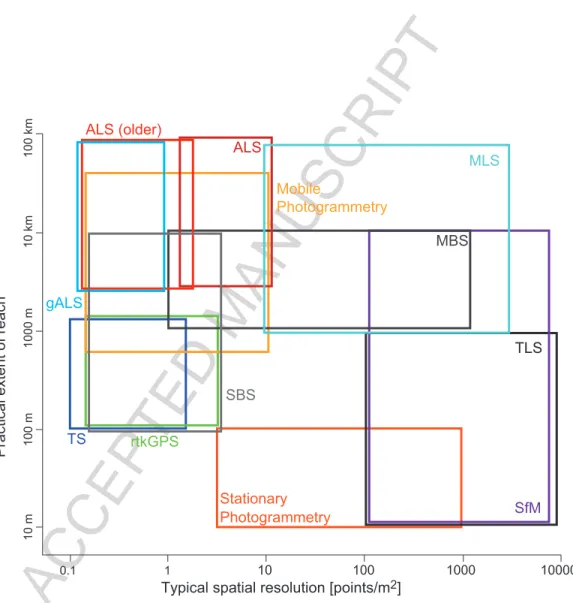
of the system being studied (Bowen and Waltermire, 2002; Lane and Chandler, 2003; Bangen et al., 2014). There are 4 main factors that control the identifica-tion of the most appropriate HRT platform and method: (i) spatial extent of the area to be acquired; (ii) point density needed to accurately represent the sur-face in analysis (and thus, horizontal and vertical measurement accuracy with
165
respect to typical spatial or temporal gradients to be captured); (iii) need for detailed representation versus elimination of vegetation and other above-ground features; (iv) capability to penetrate water and acquire bathymetry. The char-acteristics of common HRT data with respect to these factors are summarized in Fig. 1 and Table 1. When existing data are available for the area in analysis,
170
these factors can guide the assessment of whether or not the existing data are appropriate for the analysis being planned. Additional factors that contribute to the choice of HRT platform are cost and flexibility. While these are not sci-entific factors per se, they do affect the decision process, particularly in the case of analyses requiring repeated surveys.
175
2.2. Available platforms and system components
Lidar sensors have been deployed from both airborne (typically called Airborne Laser Scanning ALS) and ground-based platforms (typically called ground based lidar or Terrestrial Laser Scanning TLS). ALS is the only technique that can
ACCEPTED MANUSCRIPT
effectively penetrate the canopy to obtain information on the ground, which is
180
the main advantage of ALS with respect to other platforms. Conventional lidar systems (airborne and terrestrial) operate in the near infrared (NIR) part of the light spectrum, which is rapidly attenuated or reflected by water and therefore provides limited information in wet areas.
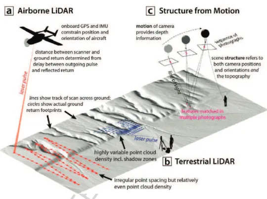
Airborne acquisition allows the ability to cover large areas (Fig. 1, Table 1,
185
Fig. 2 (a)) in small amounts of time (hours). Tripod base (TLS) is instead used when a higher resolution and more flexibility in the scanning angle are needed (Fig. 2 (b)). The spatial extent of TLS is much smaller than ALS (Table. 1, Fig. 1) and the feasible extents vary by instrument (long-range versus short-range) and geometry of the area of interest.
190
Vegetation can be very difficult to remove from ALS and TLS data and may in fact be the largest source of uncertainty in locations with moderate to high vegetation density. There are not many comparable alternatives that provide the spatial extent and point density that can be attained with ALS data (Table 1, Fig. 1), so imperfect removal of vegetation (when needed) may be an
195
acceptable cost for obtaining the HRT data of interest. On relatively small spatial scales, however, conventional rtkGPS or theodolite surveys may provide a more accurate representation of the ground surface compared with TLS.
Recently developed mobile lidar systems (MLS) include sensors mounted on mobile vehicles (including boats) (Alho et al., 2009; Vaaja et al., 2011; Williams et al.,
200
2013, 2014), compact systems portable in backpacks (Brooks et al., 2013; Glennie et al., 2013a), and mounted on Unpiloted Aerial Vehicles (UAV), kites, and blimps. Such systems blend some of the greatest benefits of ALS and TLS. The main advantages of these units are the capability of responding much faster to geo-morphic and hydrologic events and of accessing steep or challenging areas where
205
tripod-based surveying may not be possible.
Bathymetric lidar (green Airborne Laser Scanning gALS) uses the green-blue portion of the light spectrum which can penetrate water. However, even within the green-blue portion of the spectrum, the capability of detecting channel bed topography varies with water depth and turbidity (Glennie et al., 2013b). A
ACCEPTED MANUSCRIPT
good rule of thumb is that data will be acquired down to approximately the depth that can be visually seen, although recently developed systems are ex-pected to reach twice the visible depth.
Given that channels are often the most dynamic 1% of the landscape and play critical roles in mass and energy transfer in landscapes, it may be
desir-215
able to utilize sonar instruments to capture bathymetry and subsequently stitch those data into HRT data covering the terrestrial surface. Single-beam SONAR (SBS) and multibeam bathymetric SONAR (MBS) are mounted on boats or on small floating devices (preferred when navigation is limited by shallow water and/or presence of vegetation). The primary advantages of SBS are cost,
rel-220
atively low (easily manageable) data density and ease of operation in shallow water. SBS surveys tend to be adequate for monitoring relatively large geomor-phic change and coarse bathymetric surveys for 1D hydrologic modeling. MBS provides a much higher data density and captures many more of the fine-scale features (ripples, dunes, boulders, etc.), which may or may not be necessary
225
depending on the question at hand. Because of the sparser data density, SBS surveys often require interpolation between survey lines, which can introduce error into the bathymetric dataset. Another emergent bathymetric technology is interferometric sonar, which has the benefits of much wider swath width, lower sensitivity to vessel roll and wave action, and lower cost, compared to MBS.
230
Synthetic Aperture Radar (SAR) is a class of side-looking radar systems that are deployed from airborne platforms, typically mounted on an aircraft or spacecraft (Doerry and Dickey, 2004; Oliver and Quegan, 2004). SAR systems can create HRT data (with m to cm precision) using advanced echo timing techniques (Doppler processing). Interferometric SAR (IfSAR or InSAR) uses
235
the parallax (phase shift) in two different SAR images collected at different radar antenna elevation angles to generate a 3D surface with vertical resolution typically less than 1 m. Advantages of SAR include the ability to collect data during the day or night and penetrate weather and dust that might limit other remote sensing techniques.
240
ACCEPTED MANUSCRIPT
m pixel resolution; e.g., WorldView-2, Pleiades, Geoeye-1) can also be used to reconstruct digital surface models (DSM) down to 1 m spatial resolution and vertical accuracy as good as 0.5 m in the best conditions (Table 1). The current limitations in using SAR and VHR comes from the relatively high level
245
of expertise needed to process the imagery into a high quality surface model. Recent photogrammetric techniques, such as Structure from Motion (SfM) (James and Robson, 2012) and Multi-View Stereo (MVS), can be mounted on UAVs and represent a low-cost option for acquiring HRT (Fig. 2 (c)). Such approaches require relatively little training and are extremely inexpensive, and
250
thus potentially represent a methodological leap in ad hoc HRT data collec-tion (Fonstad et al., 2013). Point cloud densities with vertical and horizon-tal error on the order of cm can be achieved, although the resulting datasets may be subject to large errors due to incorrect flight plans or lens calibration (James and Robson, 2014).
255
Comprehensive reviews on each platform can be found in the literature, such as Mallet and Bretar (2009), Petrie and Toth (2009c), and Glennie et al. (2013b) (ALS including full waveform), James and Robson (2012) and Westoby et al. (2012) (SfM), Heritage and Hetherington (2007), Petrie and Toth (2009a), Petrie and Toth (2009b), Day et al. (2013a), and Day et al. (2013b) (TLS), Brooks et al. (2013),
260
Glennie et al. (2013a), and Williams et al. (2014) (MLS), Hobi and Ginzler (2012) and Stumpf et al. (2014) (VHR), Bangen et al. (2014) (SBS, MBS), and Wasklewicz et al. (2013) for an overview on ALS, TLS, photogrammetry, and SAR.
2.3. Sources of uncertainty, error modeling and error propagation
Regardless of the HRT platform, uncertainty assessments of raw HRT data and
265
subsequent post processing into point clouds, terrain and surface models should be completed and reported with any scientific study. For both the investigator and the audience, the most important question to address is whether or not the uncertainty is significant to the question or purposes for which the HRT is being used (Wheaton et al., 2008). The type of assessment and the extent
270
ACCEPTED MANUSCRIPT
one is answering. A comprehensive uncertainty analysis or full error budget can be challenging (Joerg et al., 2012) and is not always necessary. We advocate focusing the uncertainty analysis on whether the signal sought from HRT data and analyses is larger than the noise inherent in the HRT data (i.e., signal to
275
noise ratio; see following sections).
Data inventory and exploration are first steps to an uncertainty assessment. For example, in addition to the point cloud information, are there independent ancillary data such as Ground Control Points (GCPs) of elevation and vegeta-tion heights available? Visual analysis of the data, either in 2D or 3D (with
280
an immersive environment) and ideally with ancillary data such as topographic or vegetation information, may reveal both obvious (e.g., data corduroy) and subtle errors in the data (e.g., power lines confused with tree tops). In addi-tion, assessing the topographic complexity and the distribution and species of vegetation across the site will provide information about the potential spatial
285
distribution and magnitude of uncertainty in the point cloud and/or raster data (Hopkinson et al., 2005; Hodgson et al., 2005; Spaete et al., 2011). This assess-ment may include parameters such as slope, surface roughness (bare earth and vegetation), and/or vegetation height and cover derived from the point cloud and/or raster data.
290
2.3.1. Scope of uncertainties
The scope of uncertainties with respect to HRT can be overwhelming and a full accounting is beyond the scope of this paper. However, we can usefully identify three primary types of uncertainties specific to HRT data that span the full scope (Table 2): i) positional uncertainties , ii) classification uncertainties, and
295
iii) surface representation uncertainties.
HRT positional uncertainties describe the uncertainty in both the horizontal and vertical location of individual topographic points in a point cloud. The source of positional uncertainties are the sensor’s precision and accuracy, the geometry of acquisition (e.g., range and angle of incidence), and the position of
300
ACCEPTED MANUSCRIPT
combination of GPS and inertial measurement unit (IMU) systems to position and orient the sensor and yield directly globally georeferenced point clouds. Ground-based surveys from a static position (e.g., TLS or TS) can be kept in a local coordinate system with high accuracy (e.g., using fixed targets) before
305
being globally georeferenced (e.g., by knowing the GPS position of the targets). Beyond the actual precision of the sensors, this difference in georeferencing translates into a position accuracy that is an order of magnitude better for TLS (sub-cm) compared to ALS (≈ 5-10 cm). Quite importantly, the georeferencing error is unlikely to be spatially uniform due to variations in the quality of the
310
GPS/IMU positioning during a survey (Lichti and Skaloud, 2010) and actual distribution and number of targets in a static TLS survey (e.g., Bae and Lichti, 2008). Data delivered by commercial providers rarely provide the means to propagate the georeferencing errors into a spatially variable uncertainty such that a uniform georeferencing error is systematically used.
315
Beyond the georeferencing error, error inherent to the instrument (in partic-ular the angpartic-ular accuracy and range accuracy/precision) and error introduced during calibration (e.g., boresight), it is important to understand that the posi-tion uncertainty of any given point obtained by a lidar system (fixed or mobile) will depend on the scanning geometry, that is the range to the ground and the
320
incidence angle (e.g., Schaer et al., 2007; Soudarissanane et al., 2011). In the absence of a simple model to account for these effects, most studies assume a uniform position uncertainty related to instrument error and scanning geometry. For high accuracy requirements it is however possible to filter out points of high incidence angle to only keep the best measurements in the subsequent point
325
cloud analysis (e.g., Schaer et al., 2007). To our knowledge, there is no way at present to directly derive a spatially explicit error model for SfM-derived point clouds. Estimates of the accuracy of SfM point clouds have been based on a comparison with higher quality data (numerous GCPs or lidar) and have shown that the position uncertainty is of the order of 1/1000 the camera distance (e.g.,
330
James and Robson, 2012). Recent work has shown that incorrect survey organi-zation can introduce large scale deformation of the surface (James and Robson,
ACCEPTED MANUSCRIPT
2014).
HRT classification uncertainties depend on quality of the detection of bare earth and method of classification (see Section 3.2). For simple scenes without
335
vegetation, without objects obstructing the view of the surface (e.g., tripods, people, etc.), and flat ground, no uncertainty is introduced at this stage. How-ever, for more typical cases of interest to Earth scientists, with different types of vegetation (e.g., trees and grass), significant roughness (e.g., debris, pebbles) and complex topography (e.g., steep slopes, vertical surfaces such as channel
340
banks), the detection and classification of the point cloud into ground and non-ground elements can be difficult and may require significant manual val-idation/correction. The first issue is to know if the ground has actually been sampled by the sensor, or if vegetation or other objects were obscuring the measurement of the ground. In that case, characterizing uncertainty in ground
345
detection requires an estimate of vegetation height. A second issue is that many algorithms for bare earth detection have been developed for 2.5D geometry typ-ical of ALS surveys (e.g., Sithole and Vosselman, 2004; Tinkham et al., 2011) and can fail when applied in steep landscapes, or cannot be applied on ver-tical surfaces documented by TLS (e.g., cliffs, overhangs, and undercut river
350
banks) where only 3D methods can be used (Brodu and Lague, 2012). Another issue specific to change detection is the fact that rough surfaces will never be sampled identically by a scanning instrument, which means that a change will always be measured even if the surface was not modified. This change is however not significant when compared to the surface roughness (e.g., Wheaton et al.,
355
2010; Lague et al., 2013). A local measure of point cloud roughness (such as the detrended standard deviation (Brasington et al., 2012)) is thus a first order estimate of the uncertainty in the ground position in the context of change de-tection. Point density also impacts the quality of bare earth detection as the denser the point cloud, the more likely that one can correctly classify vegetation
360
and ground.
HRT surface representation uncertainties are related to the transformation of the unorganized point cloud into a continuous elevation surface. The most
ACCEPTED MANUSCRIPT
commonly used representation is a raster digital elevation model (DEM), but TINs, 2.5D meshes, and fully 3D meshing algorithms are being used with
in-365
creasing prevalence. For simple (smooth) 2D environments without vegetation and that have been densely sampled, this operation introduces very little un-certainty beyond a loss of horizontal accuracy. In complex scenes with vertical features (channel banks, cliffs), rough surfaces (debris (Schurch et al., 2011), gravel (Wheaton et al., 2010)) and wetted zones, DEM creation introduces
sev-370
eral uncertainties. First, for TLS, the more complex and rough the surface, the more likely it is that occlusion occurs such that the surface will be incompletely sampled and inappropriately interpolated during the DEM creation. This is also the case for ALS data for which wetted surfaces cannot be surveyed and typical standard interpolation by triangulation approach can result in severe artifacts
375
(e.g., Williams et al., 2014). Second, DEM creation increases horizontal uncer-tainty (up to the pixel size) and vertical unceruncer-tainty for sharp features, which results in a loss of accuracy for horizontal measures (e.g., channel width), hori-zontal change detection (e.g., channel bank erosion), and vertical change detec-tion in steep slopes (e.g., hillslope erosion). Surface representadetec-tion uncertainty
380
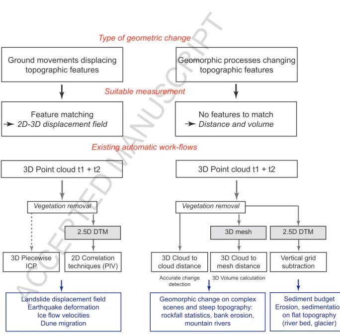
can be avoided by working directly on point clouds, especially in the context of accurate change detection on complex geometries (Lague et al., 2013).
2.3.2. Accounting for uncertainty: simple to complex
The most basic approach to HRT uncertainty accounting for Earth science ap-plications is to start simple and conservative and add complexity and
sophisti-385
cation in the error analysis only as warranted by the question of interest. For example, if HRT is to be used for geomorphic change detection of a very large magnitude signal (e.g., massive lateral retreat of a cliff face), a simple and con-servative error model may suffice because the signal will be much greater than the estimated noise. If by contrast, the geomorphic change detection is of a very
390
small magnitude (e.g., shallow sheets of deposition across a floodplain) a less conservative and more sophisticated model of error may be warranted to see if the signal can be detected and if/how the pattern varies spatially.
ACCEPTED MANUSCRIPT
A second principle of HRT uncertainty accounting and error estimation is that a more sophisticated model of error cannot reduce the uncertainty, just
395
more accurately quantify it (Wheaton et al., 2010). That is, it makes sense to invest time in a more sophisticated model when there is reason to believe that the data is fundamentally of high enough quality and accuracy to reveal the HRT-derived signal of interest. This is not necessarily known a priori, but general rules of thumb as highlighted in the best case error magnitudes of
400
Table 2 can give some lower plausible bounds on what is possible depending on the survey technique. However, a more accurate estimate of HRT errors may simply highlight locations where the signal is indistinguishable from noise. This in itself may be helpful for identifying primary sources of error worth attempting to constrain or rectify in future HRT data acquisition or post processing, but for
405
any existing HRT dataset or derivative it cannot convert poor quality data to good quality data. For example, if the signal is obscured by noise, considering the classification uncertainty or positional uncertainty in more detail may help identify if fundamental problems exist in the raw data (e.g., GPS positioning was inaccurate) or in what was surveyed (e.g., are there any ground shots in the
410
TLS survey?) that cannot be rectified, or if they may be other problems that more sophisticated post-processing may rectify (e.g., flight line misalignment or incorrect vegetation versus ground classification).
Finally, it is important to remember that the estimation of HRT error needs to be done independently for each survey. Many HRT analyses are based entirely
415
off a single survey, at one point in time, with one acquisition/platform/method. It goes without saying that the uncertainty in subsequent HRT analyses are a function of the errors in that survey. However, some HRT models may be a hybrid product of multiple types of HRT surveys, or a composite of HRT surveys from multiple points in time (e.g., an ALS survey of hillslopes and
420
valley bottom from one point in time with a more recent MBS survey of the channel bathymetry). Similarly, any geomorphic change detection problem in-volves HRT surveys from at least two points in time, and the subsequent un-certainty will be based on independently estimated errors for each HRT survey
ACCEPTED MANUSCRIPT
that are propagated into each other. Most use simple error propagation methods
425
(Taylor, 1997) which propagate independently estimated errors for each survey (in case of change detection) using the square root of sum of errors in quadrature (Lane et al., 2003; Brasington et al., 2003). For example, to estimate the total
propagated error in a DEM of Difference calculation (σDoD), the estimates of
errors in the new DEM (σDEMnew) and the old DEM (σDEMold) are combined
430 using: σDoD= q σ2 DEMold+ σ 2 DEMnew (1)
Below we highlight five situations using HRT data that span from the sim-plest error modeling to full error budgeting. The examples primarily apply to the estimation of vertical errors in a surface model, but the principles are the same whether describing horizontal or vertical errors for cells in a surface or
435
individual points in a point cloud.
1. Situations where spatially uniform may be enough
A spatially uniform error estimate assumes that σ is not a function of lo-cation and is constant in space. A spatially uniform error assessment may be sufficient where the signal that one aims to obtain is large relative to
440
the uncertainty. As an example, a study in which an ALS dataset is used to differentiate target features on the order of meters, a spatially uniform accounting of the error may be sufficient. In this example, visual exam-ination of the data for offset between flight lines, analyzing independent GCPs of the data, and analyzing the topographic and vegetation
complex-445
ity may be sufficient to assume the reported error by the vendor (e.g., +/-15 cm). Note that spatially uniform error estimates that are derived from independent check point data that span the whole range of conditions sur-veyed are strongly preferable to those just done in the simplest and easiest conditions (e.g., check points on the airport runway). If independent check
450
points were not surveyed, but the HRT survey overlaps a previous survey, which used the same ground control network and coordinate system,
us-ACCEPTED MANUSCRIPT
ing fiducial (or reference) surfaces in areas that have not changed (e.g., bedrock outcrops) can be used as an alternative (Klapinski et al., 2014). 2. Situations where simple zonal spatially uniform may suffice
455
There are a variety of situations where using a single spatially uniform value to estimate vertical surface representation errors will be overly con-servative in some areas and overly liberal in other areas (Wheaton et al., 2008). A simple improvement can come from defining regions (i.e., poly-gons) within which it is reasonable to assume σ is constant. For
exam-460
ple, Lane and Chandler (2003) identified differences in σ on the basis of whether the surface was wet or dry. Others have differentiated ALS DEM errors on the basis of vegetated or unvegetated. Klapinski et al. (2014) dif-ferentiated regions in hybrid HRT surveys on the basis of survey methods and roughness (e.g., TS, MBS - rough, MBS - smooth, ALS).
465
3. Situations where statistical error models make sense
Statistical error modeling of both surface representation uncertainty and point clouds are possible when HRT point clouds are sufficiently dense to calculate meaningful statistics. Such statistics can be calculated for all the points that fall within a moving window centered on sample points
470
(i.e., point-cloud based), or within a grid cell (i.e., surface representation uncertainty). For elevation statistics to be meaningful, they should be calculated only where 4 or more points exist in the sample window or cell. Typical statistics include zMin, zMax, zMean, zRange and zStdDev. Such statistics can be heavily skewed by local surface slope. Brasington et al.
475
(2012) developed a method to fit a mean surface through each grid cell and then recalculate detrended statistics. For example on a reasonably sloping surface comprised of cobbles and/or boulders, the standard deviation of elevation may be more a reflection of the relief and slope across that cell, whereas the detrended standard deviation is a proxy for the surface
rough-480
ness. In fact Brasington et al. (2012) found a tight correlation between grain size, surface roughness, and standard deviation. For HRT survey
ACCEPTED MANUSCRIPT
methods like TLS, SfM, and MBS, individual point accuracy is generally very high and surface roughness is often the dominant driver of surface representation uncertainties and is a reasonable first cut itself as an
er-485
ror model. Brasington et al. (2012) developed the ToPCAT (Topographic Point Cloud Analysis Tool) to facilitate these calculations.
In very dense point clouds, it is not uncommon to have 100’s to 1000’s of coincident points (points that have different z ’s but share the same x and
y coordinates). Hensleigh (2014) used the overlap in MBS boat passes
490
(analogous to ALS flight lines) to calculate coincident points as a proxy for measurement uncertainty.
Another approach to statistical estimation of errors is bootstrapping. Us-ing this approach, an elevation surface is built with some random fraction of the data (e.g., 90% of points) and the remaining points (e.g., 10%)
495
are used to calculate residual errors between the interpolated surface and measured points (Wheaton et al., 2008). Those residual error value points can be interpolated to approximate an error surface. The process can be repeated multiple times with different random samples to increase the density of points in the interpolated error surface. Note that the
result-500
ing distribution of residual errors is sometimes used to estimate spatially uniform errors across an entire surface or within zones.
4. Situations where more complicated spatially variable error models are
war-ranted
Although the statistical error models described above are spatially
vari-505
able, there may be other factors important in determining the surface uncertainties than just simple elevation statistics. For example, angle of incidence, footprint size, topographic complexity of the surface, sampling density, positional point quality, and interpolation error may all trump sur-face roughness as the primary driver of error in certain localities within an
510
HRT survey. In these cases, spatially variable error models are warranted. For these studies, one can expand upon the error analysis above.
Assum-ACCEPTED MANUSCRIPT
ing the point cloud data are available, assessing the spatial relationship between slope, roughness, and vegetation height and cover may be nec-essary. This can be completed by developing statistical relationships
be-515
tween independent GCPs and these parameters, using a machine learning approach such as RandomForest (Breiman, 2001). Milan et al. (2011) re-viewed some of the approaches available for estimating spatially variable errors. For example, fuzzy inference systems provide a convenient way of combining multiple lines of evidence and the outputs can be calibrated to
520
independent statistical models of error (Wheaton et al., 2010). All of the above methods are supported in the Wheaton et al. (2010) Geomorphic Change Detection Software (GCD: http:\gcd.joewheaton.org). 5. Situations where full error budgets are warranted
Sometimes, if none of the cases described above applies, full error
bud-525
gets may be warranted and additional information will be needed. For example, complete metadata, including SBET (Smoothed Best Estimate of Trajectory) information of the data collection, will allow for analysis of error in relation to flight parameters such as scan angle, and use of inten-sity data to identify the relationship between error and ground/vegetation
530
targets (Glennie, 2007; Streutker et al., 2011). Spatially distributed inde-pendent GCPs should be collected and used to estimate the error in dif-ferent slopes and vegetation types. Perhaps one of the most mature exam-ples of full error budgeting comes from the multi-beam sonar community, where TPE (total propagated error) is used in the CUBE (Combined
Un-535
certainty Bathymetric Estimator) tools (Calder and Mayer, 2003) to esti-mate uncertainties and minimize user subjectivity when data are cleaned and filtered. The TPE estimates attempt to quantify all sources of er-rors leading to point-based estimates of uncertainty as well as surface-based estimates of uncertainties. The TPE estimates frequently result
540
in overly conservative estimates of total error, but they are none-the-less useful in reliably defining the spatial pattern of those errors, their
rela-ACCEPTED MANUSCRIPT
tive magnitudes and revealing the key sources. The downside of full error budgeting is that it requires a considerable amount of extra input data that is often not available (with the notable exception of hydrography
545
surveys in MBS). These methods are supported in most of the industry-standard MBS manufacture post-processing software (e.g., HPACK and HYSWEEP: http://www.hypack.com/).
In the context of change detection, simple tests should be performed on various parts of one of the surveys to make sure that the uncertainty model
550
is consistent with the change detection method used. For instance, com-paring two different decimations of the same point cloud should not yield a statistically detectable change given the uncertainty estimated locally as a function of point density and point cloud roughness (Lague et al., 2013). These methods are supported in the M3C2 algorithm within the
555
CloudCompare software (http://www.danielgm.net/cc/)
2.4. Summary of common sources of error in HRT analysis and questions one should ask
In Table 3 we list several common sources of error in HRT analysis and provide recommendations for each. As seen from the previous sections, there are
nu-560
merous sources of uncertainty that are commonly unknown to the user. To help designing the acquisition of new HRT data or planning the analysis of existing HRT data, we provide in Box 1 and Box 2 questions that any user should ask prior to the beginning of the project. Information on how to address most of these questions is provided in the sections that follow. Some of these questions
565
are too specific to the project at hand to be properly addressed in this review. We recommend users to collect the information needed to address each question before starting the analysis of data.
2.5. Metadata and reproducibility of scientific results
New data acquisition should follow basic criteria for data storing and sharing.
570
ACCEPTED MANUSCRIPT
and vertical accuracy must be stored with the data as well as information on how the data were further processed (e.g., point cloud decimation and classification). While some vendors prefer to keep this information proprietary and inaccessible, it is fundamental to allow reproducibility of scientific results. Helpful reviews
575
on this topic with specific rules to follow for storing and sharing data have been recently provided by White et al. (2013) and Goodman et al. (2014) and include (i) sharing data; (ii) provide metadata; (iii) provide an unprocessed form of the data; (iv) use standard format; (v) perform basic quality control.
3. DO: Working effectively with HRT data, from raw point clouds to
580
usable data and derivative products
In this section we discuss research questions of interest to the understanding of how mass and energy are transferred through landscapes and how their analysis has changed with the availability of HRT data. We also discuss important con-siderations in data processing, including segmentation and filtering, and present
585
general work-flows for feature detection and change detection, which are among the most recurrent operations performed on HRT data. While we refrain from listing available software for each operation (as software is in constant evo-lution), we refer the reader to the OpenTopography Tool Registry where an updated list of available tools is maintained as well as comments and feedback
590
from the tool users (http://www.opentopography.org/).
3.1. Science with HRT data
Viewing HRT as simply a higher resolution version of its coarser predecessors (e.g., 30 m SRTM data) greatly understates the value of these data for two primary reasons. First, HRT is typically collected at a resolution that
per-595
mits identification and measurement of the fine-scaled features that inform our understanding of the rates and mechanisms of eco-hydro-geomorphological and earthquake processes. The fact that fine-scaled features can be resolved, changes our approach for analysis and calls for a suite of new techniques and tools for
ACCEPTED MANUSCRIPT
data analysis. Secondly, most HRT datasets contain valuable information
be-600
yond the bare earth surface elevations (e.g., above ground vegetation density, variability in surface reflectance). Such information can be immensely useful for characterization of the landscape and modeling Earth surface processes.
3.1.1. HRT provides new approaches to answer fundamental questions
In the material that follows, we discuss some high level questions currently
605
being pursued by the Earth Surface and Critical Zone communities and discuss how HRT provides opportunities for entirely new approaches to answer these questions.
1. How are mass and energy transported through landscapes?
This question encompasses a wide range of studies, from understanding
610
stress and strain fields in tectonically active environments (Frankel and Dolan, 2007; Oskin et al., 2012), to using HRT-derived canopy models to estimate radiative transfer (Lefsky et al., 2002; Vierling et al., 2008; Morsdorf et al., 2009), to constraining sediment, carbon and nutrient budgets and predict-ing fluxes at the reach or watershed scale (Paola et al., 2006; Belmont et al.,
615
2011; Hudak et al., 2012; Tarolli et al., 2012). Regardless of the
spe-cific application, HRT substantially enhances our capacity to answer this question by offering precise quantification of critical features distributed throughout a large spatial domain (e.g., geometry and location of fault scarps, tree canopy, channel heads, river banks, detention basins, see
620
Pike et al. (2009)). Directing budgeting of mass redistribution provides constraints on the magnitude and spatial patterns of geomorphic and ecologic processes. Further, HRT provides a much more detailed and reliable boundary condition for eco-hydro-morphodynamic models, es-pecially insofar as it allows direct coupling with the built environment
625
(Priestnall et al., 2000) and explicit representation of surface roughness (typically dominated by vegetation) (McKean and Roering, 2004; Glenn et al., 2006; Cavalli et al., 2008; McKean et al., 2014), which, for example, has
ACCEPTED MANUSCRIPT
allowed for vast improvement in flood inundation prediction (NRC, 2007). Since HRT allows users to derive higher dimensional information about
630
the surface (e.g., surface cover, roughness), it provides an opportunity to directly link hydraulics, geomorphology, and ecology. In this way, HRT improves the accuracy, spatial extent and response time for hazard assess-ment and risk mitigation, as well as restoration and conservation planning (Farrell et al., 2013). In cases where it is not feasible or desirable to
in-635
clude all of the detailed information in a model, HRT provides a basis for upscaling localized measurements and generating sub-grid scale parame-terizations (Casas et al., 2010; Helbig and Lowe, 2012; Ganti et al., 2012). For many such applications, it is useful to utilize 3D point cloud data to retain information about the above-ground features.
640
2. What are the patterns on the Earth’s surface that can inform our
under-standing of ecologic, hydrologic, and geomorphic processes and coupling thereof ?
Understanding how topography and biota are organized at the micro-, meso-, and macro-scales has been a long standing question in Earth
sur-645
face science (e.g., Gilbert and Dutton, 1880; Dietrich and Perron, 2006; NRC, 2010). Quantifying the organization of landscape features brings us one step closer to understanding the mechanisms of landscape change (Chase, 1992; Roering, 2008; Hilley and Arrowsmith, 2008; Perron et al., 2009; Roering et al., 2010). Certain features can only be represented and
650
measured accurately/precisely at HRT scales. Therefore, we have only recently acquired the capability to answer this question over large spa-tial scales. For example, HRT provides a more detailed representation of micro-climates and micro-habitats and a bridge between atmospheric boundary layer and highly localized features/characteristics (e.g.,
temper-655
ature, soil moisture, snow depth) (Molotch et al., 2004; Galewsky et al., 2008; Galewsky, 2009; Deems et al., 2013). HRT data also allows for cou-pled 3D mapping and modeling of vegetation, hydrology, and topography
ACCEPTED MANUSCRIPT
(Ivanov et al., 2008) and in some cases captures the influence/signature of bioturbation (e.g., plants, gophers) (Yoo et al., 2011; Reed and Amundson,
660
2012; Hugenholtz et al., 2013). Lastly, HRT allows for direct identifica-tion and quantificaidentifica-tion of human imprints on the landscape, permitting distinction between the effects of natural and anthropogenic processes (Passalacqua et al., 2012).
3. How do processes in one location influence processes or rates in another
665
part of the landscape?
One of the most intriguing opportunities presented by HRT data is the ability to predict non-localized effects of processes (Anderson et al., 2012). For example, initiation of a landslide near a ridge crest is likely to cause deposition of a slug of sediment in the valley bottom. Bank erosion at one
670
or many individual locations throughout a watershed is likely to influence turbidity and sediment flux at the mouth of the watershed. Such pre-dictions can only be reliable if the critical features can be identified and the transport mechanisms between the points of interest are known. HRT provides a new mechanism for satisfying the inputs needed for detailed
675
models of mass and energy transfer and takes us a step closer to robust spatially-distributed modeling over large domains.
Improved algorithms to quantify landscape topology and conduct ensem-ble feature mensuration enaensem-ble analysis of spatial relationships, from sim-ple metrics such as distance, height, and volume to more comsim-plex
evalu-680
ations of feature proximity and transport pathways (Huang et al., 2011; May et al., 2013; Tomer et al., 2013). Such analyses require the ability to recognize discrete objects whose scale may range between slightly larger than the data resolution and something smaller than the extent of the entire dataset.
ACCEPTED MANUSCRIPT
3.1.2. Fully utilizing HRT requires new approaches, tools, and techniques
The fact that in HRT we can resolve many of the fine-scale features that are critical for eco-hydro-geomorphic processes changes our analytical ap-proach and demands a new set of tools and techniques. HRT contains an immense amount of information, much of which is not easily extracted
690
with conventional tools. The analysis challenges shift from relatively sim-ple operations performed either on individual pixels or the entire dataset, to the realm of image processing, where the richness of the image can be deconstructed into more meaningful components and manipulated accord-ingly. For example, coarse topographic datasets that have been prevalent
695
for the past few decades were limited to evaluating macro-scale features, such as basin hypsometry, slope and relief, using pixel-based approaches. Watershed and channel network delineation could only be automated using algorithms that mapped pixel-to-pixel paths of steepest descent and chan-nel heads would be somewhat arbitrarily located at some average/uniform
700
value of upstream contributing area. Small order channels were not iden-tifiable and the boundaries of large channels were poorly resolved. The presence of fine-scaled features in the HRT landscape does not entirely circumvent the need for such approaches, but does open the door to en-tirely new approaches that are able to take advantage of the wealth of
705
information provided by HRT.
For example, preservation of sharp landscape features, those which are characterized as abrupt changes in topography (e.g., streambanks or fresh fault scarps), requires the use of anisotropic filters (such as nonlinear fil-ters) for cleaning and analysis of HRT. Conventional topographic filters
710
(e.g., Gaussian) have a tendency to diffuse or altogether eliminate such features (Passalacqua et al., 2010b). Another important shift in tools and techniques between conventional topography data and HRT is the use of object-based image (Bian, 2007; Blaschke, 2010). Object-based techniques have been used extensively since the 1980s and 1990s in the industrial and
ACCEPTED MANUSCRIPT
medical fields, but have only recently emerged as useful tools for Earth sur-face science, as the resolution of satellite imagery and topographic datasets has come to exceed the scale of many of the objects, or features, of inter-est. While it is not the goal of this paper to comprehensively review all of these emerging approaches, it is important to acknowledge their growing
720
use.
Some common object based techniques include segmentation, edge-detection, and feature extraction (Alharthy and Bethel, 2002; Su´arez et al., 2005; Brennan and Webster, 2006). Segmentation involves identification of dis-tinct objects by one or more homogeneous criteria in one or more
dimen-725
sions of feature space. Clearly, objects exist across a variety of scales in HRT, and so segmentation often requires a multi-scale analysis (Hay et al., 2001; Burnett and Blaschke, 2003; Hay et al., 2003; Schmidt and Andrew, 2005; Brodu and Lague, 2012). Other techniques, such as artificial neu-ral networks (Nguyen et al., 2005; Priestnall et al., 2000), fuzzy set
meth-730
ods (Schmidt and Hewitt, 2004; Cao et al., 2011; Hofmann et al., 2011;
Hamedianfar et al., 2014), genetic algorithms (Li et al., 2013; Garcia-Gutierrez et al., 2014), machine learning (Zhao et al., 2008, 2011; Gleason and Im, 2012b,a),
and support vector machines (Mountrakis et al., 2011; Zhao et al., 2011; Brodu and Lague, 2012) also show great promise to represent discrete
fea-735
tures within complex and heterogeneous environments, but applications of such approaches for HRT analysis have been relatively few. Such ap-proaches can greatly expand our capacity to extract useful information from HRT and we thus expect them to become more prevalent in the near future.
740
3.2. Getting the data right: From raw to derivative products
Currently, the vast majority of HRT users begin their analysis work-flows with a gridded product (i.e., DEM) that has previously been subjected to extensive cleaning and filtering and perhaps manual editing (Fisher, 1997). In some cases this is an appropriate starting point for the task at hand, although users should
ACCEPTED MANUSCRIPT
be aware of the operations previously performed on the data and associated potential for bias/error, as discussed above. In other cases users may start from this point because upstream versions of the data (raw, classified, or filtered point cloud) are not made available from the data provider, a situation that is becoming less common as vendors and users recognize the value of such data.
750
In yet other cases, many users simply start with the gridded dataset because the common software packages are ill-equipped to deal with point cloud data, or are perceived to require an unwarranted investment of time and effort to utilize. However, tools for cleaning and analyzing point clouds have been improved con-siderably and, for a variety of applications, the general HRT analysis community
755
has much to gain by beginning their analysis workflow further upstream. In the material that follows, we cover the operations that are commonly performed from raw data to the creation of derivative products (such as usable point cloud and DEM). Users should require specifics on these operations from the data providers. If new HRT are collected, this information should be
com-760
piled and released with the data to facilitate data reuse and reproducibility of scientific results and allow for problems to be rectified in the future as tools for data cleaning and interpolation are improved.
3.2.1. Georeferencing
During the georeferencing operation raw data are converted from a local
coor-765
dinate frame to a geodetic coordinate frame using direct and indirect methods. Direct methods imply that geodetic coordinates have been collected and assigned to positions on the ground at the time of data acquisition. A terres-trial example is ground-based rtkGPS surveying where topographic points are assigned x,y,z coordinates in real time. Accuracy of such surveys is greatly
en-770
hanced when users post-process the data to obtain differentially corrected static GPS measurements. This can be achieved using, for example, the Online Po-sitioning User Service (OPUS) to tie GPS positions collected using an antenna and local base station to the U.S. National Spatial Reference System from nearby Continuously Operating Reference Stations (http://www.ngs.noaa.gov/OPUS/).
ACCEPTED MANUSCRIPT
Similar post-processing tools are freely available from a variety of other sources on the web.
Aerial and mobile direct methods are based on the exterior orientation of the sensor relative to the Earth, which can be obtained using GPS and an Internal Navigation System (INS) (Legat, 2006). Geodetic coordinates of
po-780
sitions in the scene are extrapolated from sensor x -y positions and altitudes. This method is most common for ALS and mobile mapping systems as well as stereo-photogrammetry flown by a manned-aircraft.
Sensors, such as cameras or lasers, fixed to UAVs typically do not have on-board navigation systems sufficient for accurate geodetic positioning.
There-785
fore, indirect georeferencing methods that rely on GCPs are common. GCPs are on-the-ground features (natural or artificial) with known coordinates that are identifiable in the collected point cloud or imagery. Typically, the positions of GCPs are surveyed close to the time of data acquisition using GPS. Georef-erencing occurs after data acquisition and can be performed easily in common
790
spatial data programs. Both error and distortion need to be considered when applying spline and polynomial georeferencing transformations.
The georeferencing operation for SfM is discussed in the next section as part of the work-flow from raw data to PC generation. For a discussion on the uncertainty associated with georeferencing see Section 2.3.1. We refer the reader
795
to Shan and Toth (2009), Vosselmann and Maas (2010), and Renslow (2012) for further reading on georeferencing.
3.2.2. Processing raw data to create a usable point cloud
In some cases it may be required to combine multiple point clouds into a single point cloud, for example in HRT surveys with point clouds obtained from
mul-800
tiple positions on a landscape. This requires bringing multiple point clouds into the same coordinate system, which may be global or local. These point clouds may be from the same HRT platform or from some combination of ALS acqui-sition, multiple TLS scans, sonar and/or cameras. Merging these point clouds into a unified dataset is achieved through a registration operation performed by
ACCEPTED MANUSCRIPT
either relying on points common to multiple clouds (minimum 3 points shared) or setting up targets during the acquisition that can then be used as reference points during the registration operation (some targets can reoccupy exactly the same position during subsequent surveys for high accuracy local georeferencing (Lague et al., 2013)). In natural scenes the latter approach is preferred as it is
810
commonly difficult to identify common points in multiple clouds and surfaces are generally rough which reduces the accuracy of cloud matching techniques (e.g., Schurch et al., 2011; Lague et al., 2013) (unlike engineering applications where features such as structure corners can be used). A lack of common targets can significantly diminish the quality of the data acquired.
815
In the case of SfM, camera pose and scene geometry are reconstructed simul-taneously using the automatic identification of recurrent features in multiple im-ages that have been taken from different angles (Snavely, 2008; Westoby et al., 2012). Although only 3 images per recurrent feature are needed, it is usually recommended to take as many photographs as possible. The point cloud is
820
created in a relative ‘image-space’ coordinate system. GCPs or physical tar-gets are commonly employed to align the ‘image-space’ to an ‘object-space’ coordinate system. The georefencing operation consists of a Helmert Trans-formation (7 parameters: 1 scale parameter, 3 translation parameters, and 3 rotation parameters) (Turner et al., 2012). Example applications can be found
825
in Westoby et al. (2012), James and Robson (2012), Javernick et al. (2014), and Johnson et al. (2014).
3.2.3. Point cloud processing, filtering, and classification
Once the point cloud has been created, several processing operations may be needed before analysis of the point cloud or creation of raster products can be
830
performed. These operations are performed to reduce the size of the point cloud, distinguish ground points from off-ground points, and classify the point cloud into homogeneous portions.
No matter what the data source is, the generated point cloud can be ex-tremely dense. In these cases the number of points often needs to be reduced
ACCEPTED MANUSCRIPT
in order to analyze the point cloud. This operation is called decimation. Proce-dures for decimation include point removal, refinement, and cloud segmentation approaches (Wasklewicz et al., 2013).
Filtering and classification are needed to distinguish ground and off-ground points and further classify the off-ground points. There are 4 main categories
840
of filtering approaches (Sithole and Vosselman, 2004; Pfeifer and Mandlburger, 2009) and they are different in the assumption they make about the structure of the ground points: (i) morphological filters (often slope-based), (ii) progressive densification filters starting from seeds (e.g., lowest points), (iii) surface-based filters (progressive removal of points that do not fit the surface model), (iv)
seg-845
mentation and clustering (operates within homogeneous segments rather than individual points). Many of these filters operate directly on the point cloud, but others require gridding to take full advantage of image processing tech-niques (e.g., segmentation). Sithole and Vosselman (2004) report results for a filter comparison on 12 different landscapes and concluded that while all filters
850
are successful in landscapes with low complexity level, the presence of urban structures or steepness influenced the performance of the filters resulting in surface-based filters (filters that rely on a parameterization of the local surface and an above buffer within which ground points are expected to be found) be-ing more successful than others. As noted by Pfeifer and Mandlburger (2009),
855
when this analysis was performed segmentation strategies had not been fully developed yet, while they have been found particularly successful in landscapes modified by humans. Further work by Meng et al. (2010) identified three types of terrain for which filtering algorithms do not work optimally: (i) rough terrains or landscapes with discontinuous slopes, (ii) areas with dense vegetation where
860
the laser cannot penetrate sufficiently, and (iii) areas with short vegetation. The classification of the point cloud, including vegetation classification, can be one of the most critical operations, particularly in natural and complex land-scapes due to the multi-scale nature of the features present. The method pro-posed by Brodu and Lague (2012) exploits this aspect by probing the surface
865